Article

A New Multi-Objective Genetic Programming Model for Meteorological Drought Forecasting

by
Masoud Reihanifar
1,2,
Ali Danandeh Mehr
3,*,
Rifat Tur
4,
Abdelkader T. Ahmed
5,
Laith Abualigah
6,7,8,9,10,11,12 and
Dominika Dąbrowska
13
1
Department of Civil and Environmental Engineering, University of California, Berkeley, CA 94720, USA
2
Department of Civil and Environmental Engineering, Technical University of Catalonia, BarcelonaTech (UPC), 08034 Barcelona, Spain
3
Department of Civil Engineering, Antalya Bilim University, 07191 Antalya, Türkiye
4
Department of Civil Engineering, Faculty of Engineering, Akdeniz University, 07058 Antalya, Türkiye
5
Civil Engineering Department, Faculty of Engineering, Islamic University of Madinah, Al Madinah 42351, Saudi Arabia
6
Computer Science Department, Al Al-Bayt University, Mafraq 25113, Jordan
7
Department of Electrical and Computer Engineering, Lebanese American University, Byblos 13-5053, Lebanon
8
Hourani Center for Applied Scientific Research, Al-Ahliyya Amman University, Amman 19328, Jordan
9
MEU Research Unit, Middle East University, Amman 11831, Jordan
10
Applied Science Research Center, Applied Science Private University, Amman 11931, Jordan
11
School of Computer Sciences, Universiti Sains Malaysia, Pulau Pinang 11800, Malaysia
12
School of Engineering and Technology, Sunway University Malaysia, Petaling Jaya 27500, Malaysia
13
Faculty of Natural Sciences, University of Silesia, Bedzinska 60, 41-200 Sosnowiec, Poland
*
Author to whom correspondence should be addressed.
Water 2023, 15(20), 3602; https://doi.org/10.3390/w15203602
Submission received: 21 September 2023 / Revised: 11 October 2023 / Accepted: 12 October 2023 / Published: 14 October 2023

Abstract

:
Drought forecasting is a vital task for sustainable development and water resource management. Emerging machine learning techniques could be used to develop precise drought forecasting models. However, they need to be explicit and simple enough to secure their implementation in practice. This article introduces a novel explicit model, called multi-objective multi-gene genetic programming (MOMGGP), for meteorological drought forecasting that addresses both the accuracy and simplicity of the model applied. The proposed model considers two objective functions: (i) root mean square error and (ii) expressional complexity during its evolution. While the former is used to increase the model accuracy at the training phase, the latter is assigned to decrease the model complexity and achieve parsimony conditions. The model evolution and verification procedure were demonstrated using the standardized precipitation index obtained for Burdur City, Turkey. The comparison with benchmark genetic programming (GP) and multi-gene genetic programming (MGGP) models showed that MOMGGP provides the same forecasting accuracy with more parsimony conditions. Thus, it is suggested to utilize the model for practical meteorological drought forecasting.

1. Introduction

Droughts are characterized by a prolonged period of below-average precipitation in a specific geographic region [1]. They have become increasingly prevalent in many regions owing to a global warming-induced increase in temperature and decrease in precipitation. Their adverse impacts on different disciplines, such as water resources, agriculture, ecology, and others, have been reported in recent studies [2,3,4]. Hence, it is a priority to monitor and forecast droughts to preserve sustainable watershed management and socioeconomic development. Accordingly, numerous studies have been conducted for drought modeling and forecasting in recent decades. To this end, different modeling and forecasting methods, such as time series analysis (e.g., [5,6,7]), regression techniques [8,9,10], and classification approaches [11,12,13], have been used. For example, Han et al. [5] demonstrated that an autoregressive integrated moving average (ARIMA) method can be applied to predict droughts in northwest China using remote sensing data. Similarly, Moghimi et al. [7] implemented ARIMA to model and forecast seasonal drought in the south of Iran. Belayneh et al. [8] developed wavelet-based artificial neural networks (ANN) and support vector regression models for long-term drought forecasts in the Awash River Basin, Ethiopia. The authors showed that the hybrid machine learning (ML) techniques outperform ARIMA in their study area. A set of ML techniques, including multivariate adaptive regression splines, least square support vector machine, and M5-Tree models, were used by [10] to model and forecast meteorological drought in eastern Australia. The study concluded that the ML models’ accuracy varies significantly according to geographic and seasonal features of drought indicators. Thus, the models may show different performances at different locations. Combining decision tree (DT) classification approaches with ANN, Vidyarthi and Jain [12] examined knowledge extraction from a meteorological drought time series in Gangetic West Bengal. The results showed that the ANN technique is suitable for one-month-ahead drought forecasting, and the rules extracted can be easily implemented as a drought forecasting tool. More recently, DT, genetic programming (GP), and gradient boosting DT (GBT) techniques were utilized by [13] for one-month-ahead prediction of meteorological drought classes in Ankara and Antalya, Turkey. The results showed that DT suffers from high variance and low generalization ability. The GBT outperformed its counterparts in both areas studied.
Several recent papers have also been conducted to review the statistical methods and ML techniques used in drought forecasting [14,15,16] and summarize the associated challenges and prospects [11,17]. Overall, the relevant literature proved that drought forecasting is a challenging task due to highly stochastic patterns existing in their representative indices. While a classic time-series analysis method or an ad hoc ML technique fails to accurately identify underlying patterns, particularly for long-term forecasts, the hybrid/ensemble ML models were preferred to do the task, indicating that there is always room for additional improvement [18,19]. Our review of the hydrological applications of ML revealed that most of the available studies have focused on increasing the forecasting accuracy, which is given less or even no attention to the rising complexity due to hybridization via adding an external optimization technique or assembling different ML techniques. Although such attempts may yield highly accurate prediction models, their extreme complexity could be a substantial obstacle to their implementation in practice. Practitioners who are interested in the use of prediction models undoubtedly prefer simpler algorithms.
Inspired by the recent improvements in multi-objective optimization theory [20,21,22], we aimed to develop an explicit parsimonious model to be employed for meteorological drought (hereafter MD) forecasting. The task was accomplished considering a well-known drought index: the Standardized Precipitation Index (SPI). The study presents a novel multi-objective model based on a state-of-the-art multi-gene genetic programming (MGGP) technique called MOMGGP, which employs Pareto front optimization theory to rank potential solutions based on their accuracy and simplicity. The Pareto diagram plots individual programs’ expressional complexity [23] vs. their error metric. To the best of the author’s knowledge, this is the first study attempting to introduce a parsimonious solution for MD prediction. The proposed model was trained and verified using data from the Burdur meteorological station in Turkey. Cross-validation was also conducted with regard to well-documented monotonical GP and multi-objective GP (MOGP) techniques.
The rest of the article is organized as follows: Section 2 elaborates on the baseline methods and the proposed methodology; the study areas and collected data/indices are described in Section 3; the attained results are discussed in Section 4; Section 5 highlights the concluding remarks with regard to the future.

2. Study Area and Data Collection

The study area is the city of Burdur (Lat: 37.72, Lon: 30.29) in the Mediterranean region of Turkey. The study area is located close to the Burdur Lake basin (Figure 1), which is one of the richest regions of Turkey in terms of surface and groundwater sources [24]. However, the increasing need for water due to widespread irrigated agricultural activities and decreasing seasonal precipitation causes drought in Burdur. The effect of the drought in the region is clearly observed in Burdur Lake, which is fed by groundwater, seasonal rainfall, and intermittent streams, such as Bozçay, Ulupınar, and Keçiborlu, discharging into the lake. Burdur Lake has been shrinking rapidly since the 1980s. With the drought experienced in the region in recent years, the ponds built on the streams discharging into Burdur Lake and the wells opened for agricultural irrigation have accelerated the decrease in the lake level. To meet the drinking water shortage in the province, recent attempts to divert the water supply from neighboring provinces are seen.
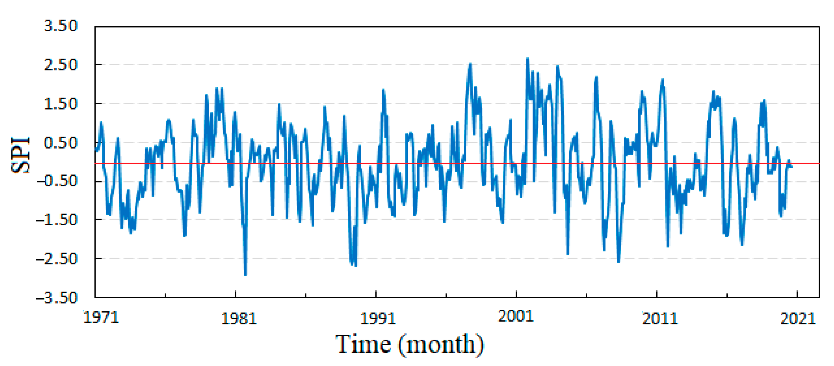
The meteorological station is located 957 m above sea level and receives about 420 mm of precipitation annually. According to long-term observations, the minimum temperature in Burdur was determined as −16.7 °C in January and the maximum temperature was 41.0 °C in July and August. During the past five decades, several moderate, severe, and extreme drought events have been reported for the study area [25]. As previously mentioned, the long-term observed precipitation data during the period from 1971 to 2021 at the station was used to calculate the SPI-6 time series (Figure 2). The data was gathered from the Turkish State Meteorological Service, and their quality was controlled before the SPI calculations.
As mentioned, 70% (30%) of the data was used to train (test) the evolved models. Both the training and testing subsets are representative of the entire data set, as is clear in Table 1. Although the SPI series is intrinsically unitless standardized data, our test runs showed the use of min–max normalization yields in more accurate forecasts. Thus, both the training and testing subsets were rescaled in the range from 0.0 to 1.0 during the models’ evolution.

3. Methods

3.1. The Standardized Precipitation Index

In this study, the SPI was used to track MD over a 6-month time frame. The underlying reason for selecting SPI-6 is that a medium-term accumulation period is more appropriate for measuring drought impacts on soil moisture and, thus, could be considered as both a meteorological and an agricultural drought signal. The SPI is widely used in the water resources engineering community for MD monitoring and prediction. The mathematical steps behind the SPI calculation on various timescales have been documented in many resources (e.g., [26]), and is commonly calculated using total monthly precipitation. First, a suitable distribution model (usually gamma function) is fitted to the precipitation time series and then transformed into a normal (Gaussian) distribution. Drought states are then categorized as listed in Table 2. The Drought Indices Calculator (DrinC) software (version 1.7) developed at the National Technical University of Athens was used to calculate the SPI in this study.

3.2. Overview of GP and MGGP

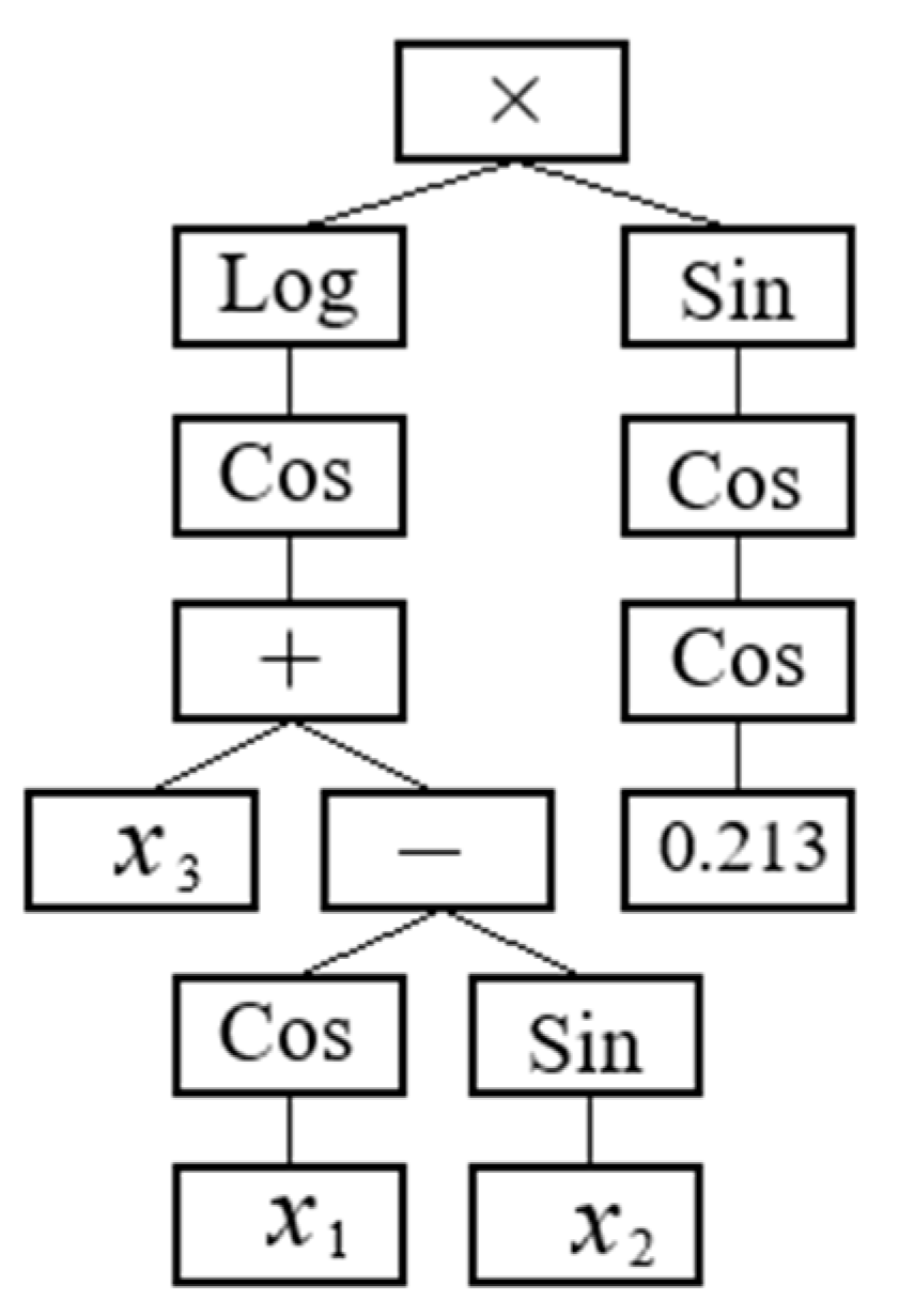
GP is an evolutionary ML technique that provides explicit and interpretable regression models [27]. Since early 2000, it has been applied in numerous hydrological prediction and forecasting studies as a robust grey box model (e.g., [28,29]). A standard GP model, aka monotonic GP, has a single tree structure (gene) comprising a root node, inner nodes, and terminal nodes (Figure 2). The nodes are connected via branches representing a mathematical expression known as a solution tree. For instance, Figure 3 illustrates a gene with a maximum depth of seven, a root node of multiplication function, and three variables (i.e., inputs: x1, x2, x3). Inner nodes are randomly filled by a user-defined function (here, Log, sin, cos, addition, subtraction, and addition). Terminal nodes are those that only can assign a variable or a constant value (here, a random value equal to 0.213). Overall, the gene expresses Equation (1) in the tree form.
y = L o g ( c o s ( x 3 + c o s x 1 s i n x 2 ) ) × s i n ( c o s ( c o s   0.213 ) )
To detect the relationship between inputs/targets, the GP algorithm starts with a random generation of the initial population of GP trees (known as potential solutions). The training process is based on reducing the error between the estimated and actual target values by adjusting the trees’ shape and elements through crossover, mutation, and reproduction operators. The best solution is commonly selected among the top three models ranked according to their accuracy. Inasmuch as the GP structure is updated at each generation, it is less likely to get stuck in the local optimum. In this study, the GPdotNet V-5 software [30] was used to model the SPI series based on training the associated historical data.
Multi-gene genetic programming (MGGP) is a new advancement of GP, so that each initial population member/potential solution consists of multiple genes. As expressed in Equation (2), the best solution is attained by a linear sum of weighted single genes plus a noise term (a0) (Danandeh Mehr and Safari 2021).
y = a 0 + a 1 G e n e 1 + a 2 G e n e 2 + + a i G e n e i
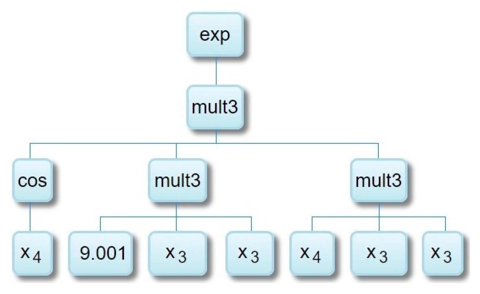
where the index i denotes the maximum number of GP trees (genes) assigned by the modeler to solve a desired problem. The coefficients a1, a2, …, ai are the regression coefficients commonly calculated using the least-square optimization technique. Figure 4 illustrates a multi-gene solution with three genes and the maximum depth of three evolved using three input variables (i.e., x1, x2, x3). Overall, the multi-gene model can be mathematically expressed by Equation (3). Eray et al. [31] demonstrated that the multi-gene GP algorithm has the potential ability to produce accurate and relatively low-depth solutions for hydrological simulations. In this study, GPTIPS [32], the MGGP toolbox, was used to develop multi-gene SPI estimation models. For more details on the monotonic GP and MGGP algorithms, and the review of their applications to solve engineering problems, the reader is referred to [30].
y = a 1   ( x 1 s i n 0.861 E x p 0.861 ) + a 2 ( 0.246 x 3 0.746 + x 1 ) + a 3 ( E x p x 2 × 0.702 ) .

3.3. State-of-the-Art MOMGGP Algorithm

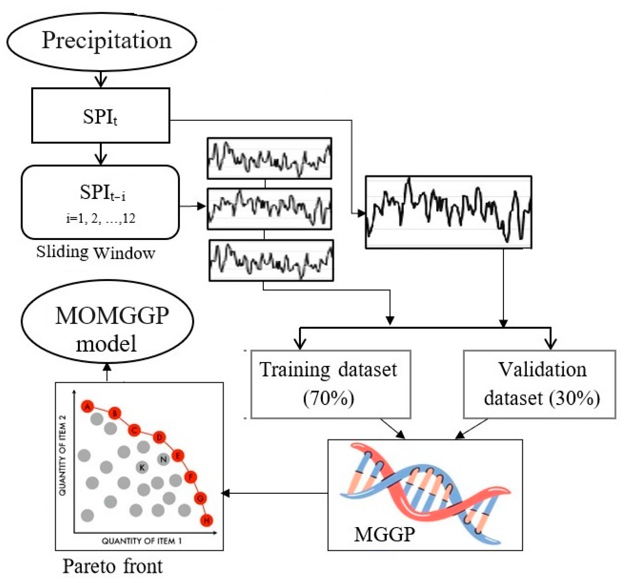
Figure 5 illustrates the proposed evolutionary MOMGGP modeling procedure for the automatic prediction of SPI with a month’s lead time. The process comprises three modules: (i) the data preprocessing module, in which the SPI datasets are reshaped into inputs/output format to be suitable for supervised learning algorithms. To this end, a sliding window method was utilized to create potential predictors for the associated label series. Here, 12 lags (i.e., previous time steps) are considered as the potential features and the current time step is considered as the label. Then, a GP/MGGP engine is run to attain the best symbolic regression models between the inputs and the target series. The evolutionary search algorithm of GP/MGGP is used as the input selection criterion to remove redundant lags that may impede the subsequent calculations and lead any ML regressor to more complicated models [33].
In the next module, the input/target series are split into train and test datasets. Here, the first 70% (the last 30%) of the data were used to train (test) the GP/MGGP models. In the last module, the multi-objective MGGP (MOMGGP) models are developed through a trade-off analysis between expressional complexity and model accuracy of MGGP solutions after 500 generations. Finally, a Pareto front plot of the potential MGGP solutions is depicted to select a parsimonious model.
To determine the degree of the complexity of a GP/MGGP model with a given maximum number of genes, the expressional complexity measure [23] was used. For example, Figure 6 illustrates a GP model possessing 4 depths, 12 nodes, and an expressional complexity of 40.

3.4. Performance Evaluation

In addition to graphical comparisons, two statistical measures were used to evaluate the performance of the models: the root mean square error (RMSE) and Nash Sutcliffe coefficient (NSE), as described below:
R M S E = i = 1 n ( S P I c S P I p ) 2 n
N S E = 1 i = 1 n ( S P I c S P I p ) 2 i = 1 n ( S P I c S P I c ¯ ) 2
where n denotes the count of months used for the training and testing phases; S P I c , S P I p and S P I c ¯ denote the observed and predicted values of the SPI and its mean value.
The RMSE shows the difference between the predicted value and the calculated SPI values, which have a value between (0, +∞), and values closer to zero indicate a higher accuracy of the forecasting model. The NSE is a dimensionless and normal parameter sensitive to limit values and takes values between (−∞, 1].

4. Results and Discussion

In this study, the SPI-6 series, which represents water balance conditions over the past 6 months, was calculated for the meteorological station using 50 years of historical precipitation records (1971–2021). The frequency of the dry spells observed (i.e., SPI-6 < 0.0) at the station revealed 295 dry events with a long-term mean of −0.81; this indicates that the station has a mild drought condition in general.

The Best GP, MGGP, and MOMGGP Solutions

GPdotNET-V5 and GPTIPS-V2 software were used to develop a monotonic GP (i.e., a single tree solution) and MGGP (i.e., a multiple tree solution) model, respectively. The main modeling attributes considered in the study are itemized below.
  • RMSE was applied as the objective function in both tools. The smaller the RMSE, the better the forecasting accuracy;
  • arithmetic operations (+, −, ×, and /), exponential function (Exp), three argument addition multiplication, square, and trigonometric functions (including sin and cos) with the same selection probability were used as arbitrary functions;
  • SPI lags (from lag 1 to lag 12) together with a set of random numbers in the range of −10 to 10 were used in the terminal set;
  • the maximum tree depth for GP and MGGP solution was set to nine and four, respectively;
  • the maximum number of genes for MGGP solution was set to five,
  • ramped half and half initialization of individuals with the population size of 300 at each run were used;
  • the run is configured to proceed for 500 generations or to terminate when a fitness (RMSE) of 0.002 is achieved.
The results of the initial GP/MGGP runs showed that the searching algorithm tends to converge quickly to an optimal solution, which presumably is the local optima. This implies that GP/MGGP deals with the highly stochastic data sets. Thus, a higher value of mutation rate (20%) was applied in the complementary runs. Thus, more diverse genetic materials were evolved at each evolution and, therefore, the GP/MGGP could overcome the problem of overfitting on the training dataset.
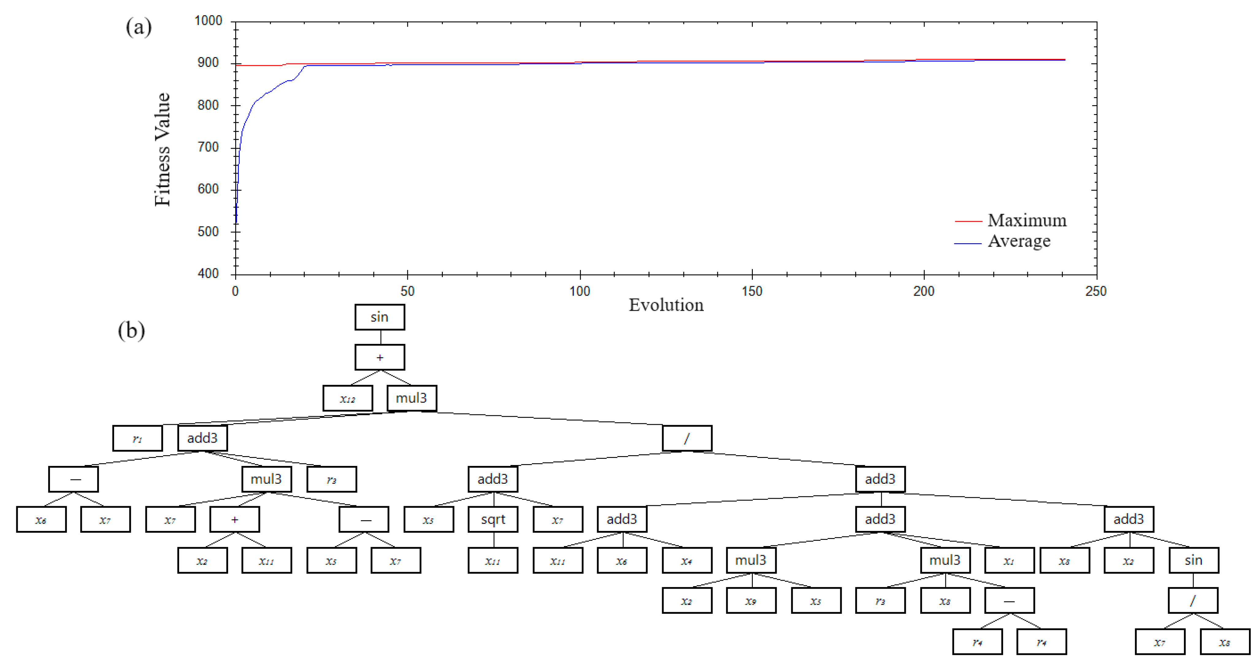
Figure 7 displays the summary of the accuracy measure of the monotonic GP models and gene expression of the best model attained for the month-ahead SPI-6 forecasting in Burdur. This figure also includes the average of all solutions (see Figure 7a) that evolved at each generation during the training period. It indicates that the initial models have weak accuracy; however, relatively accurate models are created quickly after 20 generations. The average of all models catches the maximum accuracy after approximately 80 evolutions. Thus, additional evolution (here up to 250) may increase the best model accuracy insignificantly.
The tree expression of the best GP model (See Figure 7b) demonstrates a highly nonlinear and complex model containing 48 nodes. However, the model suffers from subtrees that do not affect fitness. In the GP, such subtrees, so-called introns, occur naturally and can be trivially simplified without modifying the solution’s operation. In Figure 7b, the red dashed area shows an intron that can be replaced with 0.0. Equation (4) expresses the best simplified GP model mathematically.
S P I t = s i n ( x 12 + ( 0.683 ( x 6 x 7 + x 7 . x 2 . x 11 . x 5 x 7 + 0.181 ) x 5 + x 11 + x 7 x 11 + x 6 + x 4 + x 2 . x 9 . x 5 + x 1 + x 8 + x 2 + sin x 7 x 8 ) )
where x1 to x12 represents SPIt−12 to SPIt−1, respectively.
Figure 8 illustrates the best MGGP solution and gene weights attained for the SPI forecasting at the Burdur station. Each individual gene contains five levels. The gene weight denotes the significance degree of the associated gene with respect to its contribution to the model fitness. Since the genes are linearly combined in MGGP, low-weight genes (here, #2 and #4) could be ignored when a parsimonious solution is the goal. In analogy to the nature of precipitation, the low-performance genes at the station may represent those light rainfall events that are less effective in the total monthly precipitation value. Like the monotonic GP evolution, a summary of the accuracy measure of the MGGP that evolved indicates that the initial models have weak accuracy; however, relatively accurate models are created after 150 generations.
Table 3 lists the accuracy results of the best GP and MGGP models. While the MGGP outperformed GP during the training period, both showed more or less the same accuracy in the unseen testing datasets. Therefore, it can be concluded that either a monotonic or a multi-gene strategy may put forward similar forecasting accuracy. However, the programs are of different structural and expressional complexity that reveal a requirement for additional attention when a modeler selects the best model. Comparing the models’ inputs, we also observed that the best models were constructed with different inputs. While 1-, 2-, 5-, 6-, 7-, and 12-month lags (i.e., six input vectors) are significant predictors in MGGP, the best GP was built using 1-, 2-, 5-, 6-, 7-, 8-, 9-, 11-, and 12-month lags (i.e., nine inputs). Increasing the number of input vectors in the GP could be considered as another complexity measure that has been neglected in the present study.
According to both models’ complexity and accuracy metrics, the MGGP provides a better solution to its counterparts, and therefore, it was selected as the baseline model to evolve the multi-objective programs. To attain the MOMGGP model that represents a parsimonious solution, Pareto-front plots of the evolved MGGP population are presented in Figure 9, as explained in Section 3.3. The Figure illustrates the forecasting error (1-NSE) of the models (i.e., blue dots) on the vertical axis against its complexity on the horizontal axis. The green dots represent the Pareto-front members, and the red-circled element is the most accurate model. Therefore, the modeler could select a parsimonious model via a trade-off among the Pareto-front members. Here, we selected the brown-circled member as the parsimonious model (i.e., Pareto-optimal MOMGGP), and the associated multi-gene model, which are depicted in Figure 10. The Figure shows that the multi-objective solution contains 4 genes with a total expressional complexity of 128. The parsimonious model showed not only less complexity but also higher accuracy in the testing period (see Table 3).
To further investigate the performance of the MOMGGP model, the observed and predicted monthly SPI time series, as well as their scatter plots in both training and testing periods, are depicted in Figure 11. According to the time series plots, the MOMMGP model can capture the periodic behavior of the observed SPI series. However, it underestimates both extreme wet and extreme dry events. This point is of paramount importance when the aim is to forecast extreme events.
According to the results, the proposed parsimonious evolutionary model was found effective for short-term drought forecasting. This finding agrees with the study by Danandeh Mehr and Nourani [23], in which the Pareto-optimal GP model was suggested for rainfall–runoff prediction. Previous studies on the application of evolutionary models for drought forecasting have shown that any model with an NSE measure of greater than 0.7 in the testing period could be considered a satisfactory model [34,35]. This proves the appropriateness of the MOOGP to be applied in practice. Compared to earlier ML-based drought forecasting studies, our review showed the particular use of hybrid models for MD forecasting [36,37]. However, the proposed model remains in the category of standalone ML models, as no external optimization or preprocessing technique was employed. This is the other perfection in the proposed model that encourages its application in practice. Despite the superior performance of the MOMGGP over GP and MGGP, our study showed noticeable limitations in attaining an ideal forecast (i.e., NSE > 0.9). This is clearly due to the high nonlinear characteristics of the SPI series that make its predictability hard [37]. The relevant literature showed that data preprocessing techniques such as wavelet or variational mode decomposition may increase the accuracy of vanilla models [18,33]. However, their inclusion in the modeling process increases the solution’s complexity markedly. Further studies are required to quantify the hybrid models’ complexity that is raised through the decomposition process.
The evolved MGGP models’ complexity was limited to two structural measures. However, in the ML field, both the size and nonlinearity of the models refer to the model complexity [38]. To apply more parsimony pressure, future studies may consider additional functional complexity measures in the multi-objective optimization stage. Inasmuch as the proposed MOMGGP model was trained and tested solely for the Burdur station, the point forecasts cannot be transferred to locations far from the weather station. Following [39,40], topographic, meteorologic, and other environmental attributes, together with SPI forecasts at all stations available in the basin, could be utilized to develop a spatial distribution map of the SPI across the study area. In ungauged catchments, multi-source precipitation products could be used for SPI monitoring and prediction [41].

5. Conclusions

In this study, a new vanilla model, namely MOMGGP, was introduced for 1-month ahead forecasts of an SPI series in Burdur, Turkey. Gauge-measured precipitation data was used to attain an SPI-6 series and use it for training and validation of the new and baseline models. The proposed approach combines the Pareto-front optimization theory with a multi-gene GP concept that yields a parsimonious evolutionary model. In the proposed approach, the best prediction model is selected not only based on its accuracy but also on its simplicity. Indeed, the MOMGGP is a stepwise explicit model that could be used for practical application. Our results demonstrate that the proposed model provides a prediction accuracy of 0.721 and 0.731, respectively, in terms of NSE in the training and testing periods. This is an acceptable range for any MD prediction model. Comparing the benchmark models, the MOMGGP decreased the model complexity by up to 30%. As the goal of monotonic GP is commonly optimizing a single program, our results show that the model complexity increases dramatically after initial evolutions. This point must be considered in all GP-based hydrological models.

Author Contributions

Conceptualization, A.D.M. and R.T.; methodology, A.D.M.; software, M.R., A.T.A. and L.A.; validation, A.D.M., R.T. and D.D.; formal analysis, A.D.M., M.R. and L.A.; investigation, A.D.M., M.R. and R.T.; resources, A.D.M. and R.T.; data curation, A.D.M.; writing—original draft preparation, A.D.M. and A.T.A.; writing—review and editing, A.D.M., A.T.A. and L.A.; visualization, D.D. and L.A.; supervision, A.D.M. All authors have read and agreed to the published version of the manuscript.

Funding

This research received no external funding.

Data Availability Statement

The is available from the corresponding author upon request.

Acknowledgments

The authors appreciate three anonymous reviewers for their constructive comments on this study.

Conflicts of Interest

The authors declare no conflict of interest.

References

  1. Berbel, J.; Esteban, E. Droughts as a catalyst for water policy change. Analysis of Spain, Australia (MDB), and California. Glob. Environ. Change 2019, 58, 101969. [Google Scholar] [CrossRef]
  2. Barker, L.J.; Hannaford, J.; Chiverton, A.; Svensson, C. From meteorological to hydrological drought using standardised indicators. Hydrol. Earth Syst. Sci. 2016, 20, 2483–2505. [Google Scholar] [CrossRef]
  3. Ntano, M.M.; Busico, G.; Mastrocicco, M.; Kazakis, N. The impacts of drought on groundwater resources in the Upper Volturno basin, Southern Italy. In Proceedings of the 16th International Congress of Geological Society of Greece, Patra, Greece, 17–19 October 2022. [Google Scholar]
  4. Jehanzaib, M.; Sattar, M.N.; Lee, J.H.; Kim, T.W. Investigating effect of climate change on drought propagation from meteorological to hydrological drought using multi-model ensemble projections. Stoch. Environ. Res. Risk Assess. 2020, 34, 7–21. [Google Scholar] [CrossRef]
  5. Han, P.; Wang, P.X.; Zhang, S.Y. Drought forecasting based on the remote sensing data using ARIMA models. Math. Comput. Model. 2010, 51, 1398–1403. [Google Scholar] [CrossRef]
  6. Achite, M.; Bazrafshan, O.; Azhdari, Z.; Wałęga, A.; Krakauer, N.; Caloiero, T. Forecasting of SPI and SRI using multiplicative ARIMA under climate variability in a Mediterranean Region: Wadi Ouahrane Basin, Algeria. Climate 2022, 10, 36. [Google Scholar] [CrossRef]
  7. Moghimi, M.M.; Zarei, A.R.; Mahmoudi, M.R. Seasonal drought forecasting in arid regions, using different time series models and RDI index. J. Water Clim. Change 2020, 11, 633–654. [Google Scholar] [CrossRef]
  8. Belayneh, A.; Adamowski, J. Drought forecasting using new machine learning methods. J. Water Land Dev. 2013, 18, 3–12. [Google Scholar] [CrossRef]
  9. Yaseen, Z.M.; Ali, M.; Sharafati, A.; Al-Ansari, N.; Shahid, S. Forecasting standardized precipitation index using data intelligence models: Regional investigations of Bangladesh. Sci. Rep. 2021, 11, 3435. [Google Scholar] [CrossRef]
  10. Deo, R.C.; Kisi, O.; Singh, V.P. Drought forecasting in eastern Australia using multivariate adaptive regression spline, least square support vector machine and M5Tree model. Atmos. Res. 2017, 184, 149–175. [Google Scholar] [CrossRef]
  11. Hao, Z.; Singh, V.P.; Xia, Y. Seasonal drought prediction: Advances, challenges, and future prospects. Rev. Geophys. 2018, 56, 108–141. [Google Scholar] [CrossRef]
  12. Vidyarthi, V.K.; Jain, A. Knowledge extraction from trained ANN drought classification model. J. Hydrol. 2020, 585, 124804. [Google Scholar] [CrossRef]
  13. Danandeh Mehr, A. Drought classification using gradient boosting decision tree. Acta Geophysica 2021, 69, 909–918. [Google Scholar] [CrossRef]
  14. Mishra, A.K.; Singh, V.P. Drought modeling—A review. J. Hydrol. 2011, 403, 157–175. [Google Scholar]
  15. Anshuka, A.; van Ogtrop, F.F.; Willem Vervoort, R. Drought forecasting through statistical models using standardised precipitation index: A systematic review and meta-regression analysis. Nat. Hazards 2019, 97, 955–977. [Google Scholar] [CrossRef]
  16. Fung, K.F.; Huang, Y.F.; Koo, C.H.; Soh, Y.W. Drought forecasting: A review of modelling approaches 2007–2017. J. Water Clim. Change 2020, 11, 771–799. [Google Scholar] [CrossRef]
  17. AghaKouchak, A.; Pan, B.; Mazdiyasni, O.; Sadegh, M.; Jiwa, S.; Zhang, W.; Love, C.A.; Madadgar, S.; Papalexiou, S.M.; Davis, S.J.; et al. Status and prospects for drought forecasting: Opportunities in artificial intelligence and hybrid physical–statistical forecasting. Philos. Trans. R. Soc. A Math. Phys. Eng. Sci. 2022, 380, 20210288. [Google Scholar] [CrossRef]
  18. Danandeh Mehr, A.; Reihanifar, M.; Alee, M.M.; Vazifehkhah Ghaffari, M.A.; Safari MJ, S.; Mohammadi, B. VMD-GP: A New Evolutionary Explicit Model for Meteorological Drought Prediction at Ungauged Catchments. Water 2023, 15, 2686. [Google Scholar] [CrossRef]
  19. Yalçın, S.; Eşit, M.; Çoban, Ö. A new deep learning method for meteorological drought estimation based-on standard precipitation evapotranspiration index. Eng. Appl. Artif. Intell. 2023, 124, 106550. [Google Scholar] [CrossRef]
  20. Xu, X.; Lin, Z.; Li, X.; Shang, C.; Shen, Q. Multi-objective robust optimisation model for MDVRPLS in refined oil distribution. Int. J. Prod. Res. 2022, 60, 6772–6792. [Google Scholar] [CrossRef]
  21. Cao, B.; Zhao, J.; Gu, Y.; Ling, Y.; Ma, X. Applying graph-based differential grouping for multiobjective large-scale optimization. Swarm Evol. Comput. 2020, 53, 100626. [Google Scholar] [CrossRef]
  22. Cao, B.; Zhao, J.; Yang, P.; Gu, Y.; Muhammad, K.; Rodrigues, J.J.P.C.; de Albuquerque, V.H.C. Multiobjective 3-D Topology Optimization of Next-Generation Wireless Data Center Network. IEEE Trans. Ind. Inform. 2020, 16, 3597–3605. [Google Scholar] [CrossRef]
  23. Danandeh, M.e.h.r.; Nourani, V. A Pareto-optimal moving average-multigene genetic programming model for rainfall-runoff modelling. Environ. Model. Softw. 2017, 92, 239–251. [Google Scholar] [CrossRef]
  24. Tercan, E.; Dereli, M.A.; Tapkın, S. A GIS-based multi-criteria evaluation for MSW landfill site selection in Antalya, Burdur, Isparta planning zone in Turkey. Environ. Earth Sci. 2020, 79, 246. [Google Scholar] [CrossRef]
  25. Soylu Pekpostalci, D.; Tur, R.; Danandeh Mehr, A.; Vazifekhah Ghaffari, M.A.; Dąbrowska, D.; Nourani, V. Drought monitoring and forecasting across Turkey: A contemporary review. Sustainability 2023, 15, 6080. [Google Scholar] [CrossRef]
  26. McKee, T.B.; Doesken, N.J.; Kleist, J. The relationship of drought frequency and duration to time scales. In Proceedings of the 8th Conference on Applied Climatology 1993, Anaheim, CA, USA, 17–22 January 1993; Volume 17, pp. 179–183. [Google Scholar]
  27. Koza, J.R. Genetic Programming as a Means for Programming Computers by Natural Selection. Stat Comput 1994, 4, 87–112. [Google Scholar] [CrossRef]
  28. Tür, R. Maximum wave height hindcasting using ensemble linear-nonlinear models. Theor. Appl. Climatol. 2020, 141, 1151–1163. [Google Scholar] [CrossRef]
  29. Herath HM, V.V.; Chadalawada, J.; Babovic, V. Genetic programming for hydrological applications: To model or to forecast that is the question. J. Hydroinform. 2021, 23, 740–763. [Google Scholar] [CrossRef]
  30. Hrnjica, B.; Danandeh Mehr, A. Optimized Genetic Programming Applications: Emerging Research and Opportunities; IGI Global: Hershey, PA, USA, 2018; p. 310. [Google Scholar] [CrossRef]
  31. Eray, O.; Mert, C.; Kisi, O. Comparison of multi-gene genetic programming and dynamic evolving neural-fuzzy inference system in modeling pan evaporation. Hydrol. Rese. 2018, 49, 1221–1233. [Google Scholar] [CrossRef]
  32. Searson, D.P. GPTIPS 2: An Open-Source Software Platform for Symbolic Data Mining. In Handbook of Genetic Programming Applications; Springer: Berlin/Heidelberg, Germany, 2015; pp. 551–573. [Google Scholar] [CrossRef]
  33. Liu, Q.Y.; Li, D.Q.; Tang, X.S.; Du, W. Predictive Models for Seismic Source Parameters Based on Machine Learning and General Orthogonal Regression Approaches. Bull. Seismol. Soc. Am. 2023. [Google Scholar] [CrossRef]
  34. Omidvar, E.; Tahroodi, Z.N. Evaluation and prediction of meteorological drought conditions using time-series and genetic programming models. J. Earth Sys. Sci. 2019, 128, 73. [Google Scholar] [CrossRef]
  35. Khan MM, H.; Muhammad, N.S.; El-Shafie, A. Wavelet based hybrid ANN-ARIMA models for meteorological drought forecasting. J. Hydrol. 2020, 590, 125380. [Google Scholar] [CrossRef]
  36. Alquraish, M.; Ali Abuhasel, K.; SAlqahtani, A.; Khadr, M. SPI-Based Hybrid Hidden Markov–GA, ARIMA–GA, and ARIMA–GA–ANN Models for Meteorological Drought Forecasting. Sustainability 2021, 13, 12576. [Google Scholar] [CrossRef]
  37. Gholizadeh, R.; Yılmaz, H.; Danandeh Mehr, A. Multitemporal Meteorological Drought Forecasting Using Bat-ELM. Acta Geophysica 2022, 70, 917–927. [Google Scholar] [CrossRef]
  38. Zhu, C. Machine Reading Comprehension: Algorithms and Practice; Elsevier: Amsterdam, The Netherlands, 2021. [Google Scholar]
  39. Yang, D.; Qiu, H.; Ye, B.; Liu, Y.; Zhang, J.; Zhu, Y. Distribution and Recurrence of Warming-Induced Retrogressive Thaw Slumps on the Central Qinghai-Tibet Plateau. J. Geophys. Res. Earth Surface 2023, 128, e2022JF007047. [Google Scholar] [CrossRef]
  40. Chen, J.; Liu, Z.; Yin, Z.; Liu, X.; Li, X.; Yin, L.; Zheng, W. Predict the effect of meteorological factors on haze using BP neural network. Urban Clim. 2023, 51, 101630. [Google Scholar] [CrossRef]
  41. Wu, X.; Feng, X.; Wang, Z.; Chen, Y.; Deng, Z. Multi-source precipitation products assessment on drought monitoring across global major river basins. Atmos. Res. 2023, 295, 106982. [Google Scholar] [CrossRef]
Figure 1. Burdur Saline Lake basin in southwest Turkey.
Water 15 03602 g001
Figure 2. The SPI-6 time series was calculated using historical precipitation records at the observatory station in Burdur, Turkey.
Water 15 03602 g002
Figure 3. An example of a standard GP tree.
Water 15 03602 g003
Figure 4. An example of an MGGP solution with tree genes.
Water 15 03602 g004
Figure 5. Schematic view of the proposed MOMGGP model.
Water 15 03602 g005
Figure 6. An example of the GP model possessing an expressional complexity of 40.
Water 15 03602 g006
Figure 7. (a) Summary of the GP runs and (b) the best GP model developed for month-ahead SPI-6 forecasting at the Burdur meteorological station.
Water 15 03602 g007
Figure 8. Multi-gene expression and gene weights of the best MGGP model developed for month-ahead SPI forecasting at Burdur. The xi (i = 1, 2, …, and 12) is the normalized lagged SPI vectors used to forecast the normalized SPI.
Water 15 03602 g008
Figure 9. The Pareto-front plot of the 300 generated MGGP models in terms of their forecasting error and expressional complexity.
Water 15 03602 g009
Figure 10. Multi-gene expression and gene weights of the proposed MOMGGP model developed for month-ahead SPI forecasting in Burdur. The xi (i = 1, 2, 3, …,12) is the normalized lagged SPI vectors used to forecast normalized SPI.
Water 15 03602 g010
Figure 11. Observed and predicted monthly SPI-6 time series and their scatter plots in the training (upper panels) and testing (lower panels) datasets.
Water 15 03602 g011
Table 1. Statistical characteristics of the SPI-6 series attained at Burdur station during the 1971–2021 period.
StationDatasetMeanMinMaxSD *
BurdurEntire0.00−2.912.651.005
Training0.02−2.912.650.987
Testing−0.04−2.582.201.046
* SD: standard deviation.
Table 2. Classifications of drought states with the aid of the SPI [26].
StateThreshold
No drought0.0 ≤ SPI
Mild drought−1.0 ≤ SPI ≤ 0.0
Moderate drought−1.5 ≤ SPI < −1.0
Severe drought −2.0 ≤ SPI < −1.5
Extreme droughtSPI < −2.0
Table 3. The performance metrics of the applied predictive models at each station.
TrainingTesting
ModelsComplexityRMSENSERMSENSE
GP1900.5500.6890.5480.726
MGGP1950.5040.7400.5550.717
MOGGP1280.5220.7210.5420.731
Disclaimer/Publisher’s Note: The statements, opinions and data contained in all publications are solely those of the individual author(s) and contributor(s) and not of MDPI and/or the editor(s). MDPI and/or the editor(s) disclaim responsibility for any injury to people or property resulting from any ideas, methods, instructions or products referred to in the content.