Stochastic Precipitation Generation for the Xilingol League Using Hidden Markov Models with Variational Bayes Parameter Estimation

Abstract

Precipitation modeling holds significant importance in various fields such as agriculture, animal husbandry, weather derivatives, hydrology, and risk and disaster preparedness. Stochastic precipitation generators (SPGs) represent a class of statistical models designed to generate synthetic data capable of simulating dry and wet precipitation stretches for a long duration. The construction of Hidden Markov Models (HMMs), which treat latent meteorological circumstances as hidden states, is an efficient technique for simulating precipitation. Considering that there are many choices of emission distributions used to generate positive precipitation, the characteristics of different distributions for simulating positive precipitation have not been fully explored. The paper includes a simulation study that demonstrates how the Pareto distribution, when used as the distribution for generating positive precipitation, addresses the limitations of the exponential and gamma distributions in predicting heavy precipitation events. Additionally, the Pareto distribution offers flexibility through adjustable parameters, making it a promising option for precipitation modeling. We can estimate parameters in HMMs using forward–backward algorithms, Variational Bayes Expectation-Maximization (VBEM), and Stochastic Variational Bayes (SVB). In the Xilingol League, located in the central part of the Inner Mongolia Autonomous Region, China, our study involved data analysis to identify crucial locations demonstrating a robust correlation and notable partial correlation between the Normalized Difference Vegetation Index (NDVI) and annual precipitation. We performed fitting of monthly dry days ratios and monthly precipitation using seasonal precipitation and year-round precipitation data at these crucial locations. Subsequently, we conducted precipitation predictions for the daily, monthly, and annual time frames using the new test dataset observations. The study concludes that the SPG fits the monthly dry-day ratio better for annual daily precipitation data than for seasonal daily precipitation data. The fitting error for the monthly dry day ratio corresponding to annual daily precipitation data is 0.053 (exponential distribution) and 0.066 (Pareto distribution), while for seasonal daily precipitation data, the fitting error is 0.14 (exponential distribution) and 0.15 (Pareto distribution). The exponential distribution exhibits the poorest performance as a model for predicting future precipitation, with average errors of 2.49 (daily precipitation), 40.62 (monthly precipitation), and 130.40 (annual precipitation). On the other hand, the Pareto distribution demonstrates the best overall predictive performance, with average errors of 0.69 (daily precipitation), 34.69 (monthly precipitation), and 66.42 (annual precipitation). The results of this paper can provide decision support for future grazing strategies in the Xilingol League.

1. Introduction

Stochastic weather generators are a family of statistical models that serve to produce random simulations with statistical properties resembling those of actual weather data [1,2]. Weather generators have the benefit of generating time series of any length, which can serve to interpolate missing historical weather data or to create future weather scenarios. The data generated by the weather generator can serve to simulate watershed hydrology, ecology, and crop growth. Precipitation, temperature, wind speed, relative humidity, and air pressure constitute the bulk of the weather information produced by weather generators. Among them, precipitation data is the most significant variable in various simulation applications due to its high spatial and temporal discontinuity [3] but also the most challenging to simulate. Therefore, the stochastic generator simulation of precipitation has been a hot research topic.

Establishing HMMs is a well-liked method for working with sequential data because of their capacity to estimate and comprehend the underlying states of comparatively succinct models. Developed and explored since the late 1960s [4], HMMs are an attractive class of models frequently used for constructing SPGs. HMMs depict generating a sequence of hidden states from an underlying Markov chain, followed by observations from each state, resulting in a sequence of observable data points. The Markov property of the state process captures temporal dependencies in the data, while the emission process at each time step characterizes spatial patterns within the data. The foundational work by Hughes and Guttorp [5] introduced the use of HMMs for fitting daily precipitation, which later evolved into non-homogeneous HMMs [6,7,8]. In non-homogeneous HMMs, the transition probabilities of the Markov process within the HMM vary with time, allowing for more flexible modeling. Bellone et al. [9] presented different emission distributions for precipitation amounts and precipitation occurrence models. Li et al. [10] conducted an analysis using daily precipitation data from 47 stations spanning from 1961 to 2009 on the Chinese Loess Plateau. Their study focused on the performance assessment of six different precipitation probability distributions: exponential, gamma, Weibull, skewed normal, mixed exponential, and hybrid exponential/generalized Pareto distributions. The results indicated that the first-order Markov chain model was generally suitable for simulating daily precipitation occurrence. Moreover, distribution functions with more parameters performed better than those with fewer parameters [10]. Breinl et al. [11] used the stochastic multi-site precipitation generator TripleM (Multisite Markov Model) to simulate precipitation patterns and conducted a review of applications related to the SPG approaches. The statistical analysis of such large-scale datasets requires parameter estimation techniques that are computationally effective and adequately capture the dynamism of the underlying processes. The maximum likelihood-based Baum–Welch algorithm is an unsupervised learning algorithm that leverages the model’s Markov assumptions for efficient parameter estimation in HMMs. However, it may encounter problems when dealing with large datasets with intricate connections. Particularly with complex structural models, it may result in overfitting problems [12]. Holsclaw et al. [13] modeled daily precipitation using a Bayesian technique; however, Gibbs sampling-based Bayesian alternatives [14] are typically computationally expensive.

As gridded remote sensing data, which tend to be highly correlated, become more easily available, Variational Bayes (VB) is considered an attractive alternative for parameter estimation. VB is scalable and can incorporate prior information. Blei et al. [15] provided a review of VB methods. However, while there is a large amount of literature on VB estimation implemented for state space models and HMM models [16,17,18,19,20], these studies usually focus only on precipitation-positive distributions as a Gaussian distribution or a mixture of Gaussian distributions. Kroiz et al. [21] determined the optimal parameter configuration of the model by comparing the BIC scores when HMMs follow exponential and gamma distributions for positive precipitation under different numbers of states and mixture components, respectively, and by combining the background of the actual problem. Then, Majumder et al. [22] outlined VB estimation for HMMs with semi-continuous emission and constructed an SPG for daily precipitation using a combination of two exponential distributions. Stochastic Variational Bayes (SVB), which employs stochastic optimization principles and a Stochastic Variational inference (SVI) algorithm, can further increase the efficiency of parameter estimation. Hoffman et al. [23] provided a review of the SVI algorithm. Foti et al. [24] developed the SVI algorithm to learn the parameters of HMMs in a time-dependent data setting. In this paper, we assume that the precipitation data of each year has the same hidden weather state characteristics, i.e., exchangeability. We employ a stochastic gradient optimization approach to sample data randomly. Subsequently, we duplicate and fill the sampled data, enabling us to iterate parameter estimation using small batches of data. This innovative approach significantly enhances the efficiency of parameter estimation when compared to the traditional VBEM algorithm.

Conducting an in-depth study of precipitation patterns in the Xilingol League is essential for implementing a flexible grazing strategy in the region and ensuring the sustainable use of its grasslands. Existing studies have mainly focused on stochastic simulation of daily precipitation data during the rainy season [21,22], which has confirmed to a certain extent the rationality of SPGs for daily precipitation simulation. However, the stochastic simulation of annual daily precipitation data has not received due attention, and the study of the emission distribution used to generate positive precipitation in HMM is also lacking. Compared to prior research, this paper takes a quantitative approach to compare the traditional exponential and gamma distribution models with the introduction of the Pareto distribution featuring a stratified structure for generating positive precipitation. We employ the VB method for parameter estimation and elucidate the characteristics and advantages of each distribution model for generating precipitation data. Compared with the exponential and gamma distributions, the Pareto distribution model is more advantageous for simulating heavy precipitation events. The reason is that the Pareto distribution model can additionally set the probability interval of uniform distribution generating random numbers in the precipitation generation model according to the overall trend of precipitation, which directly determines the upper limit of the precipitation sequence, i.e., the maximum value of single-day precipitation. In this paper, building on the analysis of daily precipitation during the rainy season, we extend the functionality of the SPG to enable its efficient application in the stochastic simulation of annual daily precipitation data.

Our primary research objectives are as follows: (1) explore the different characteristics of different emission distributions in simulating positive precipitation; (2) compare the performance gap between the VBEM algorithm and SVB algorithm as parameter estimation methods for precipitation simulation; (3) compare the performance difference of SPG in simulating daily precipitation during the rainy season and annual daily precipitation; (4) perform annual precipitation prediction on three selected sites in the Xilingol League. Practically speaking, the SPG in this paper can generate daily precipitation time series data of arbitrary length, based on which the frequency and intensity data of monthly precipitation can be obtained. We could emphasize the significance of such data, especially for specific plants with brief growth cycles. Generally speaking, the SPG can aid in addressing practical issues that involve simulating and predicting daily, monthly, and annual precipitation.

2. Materials and Methods

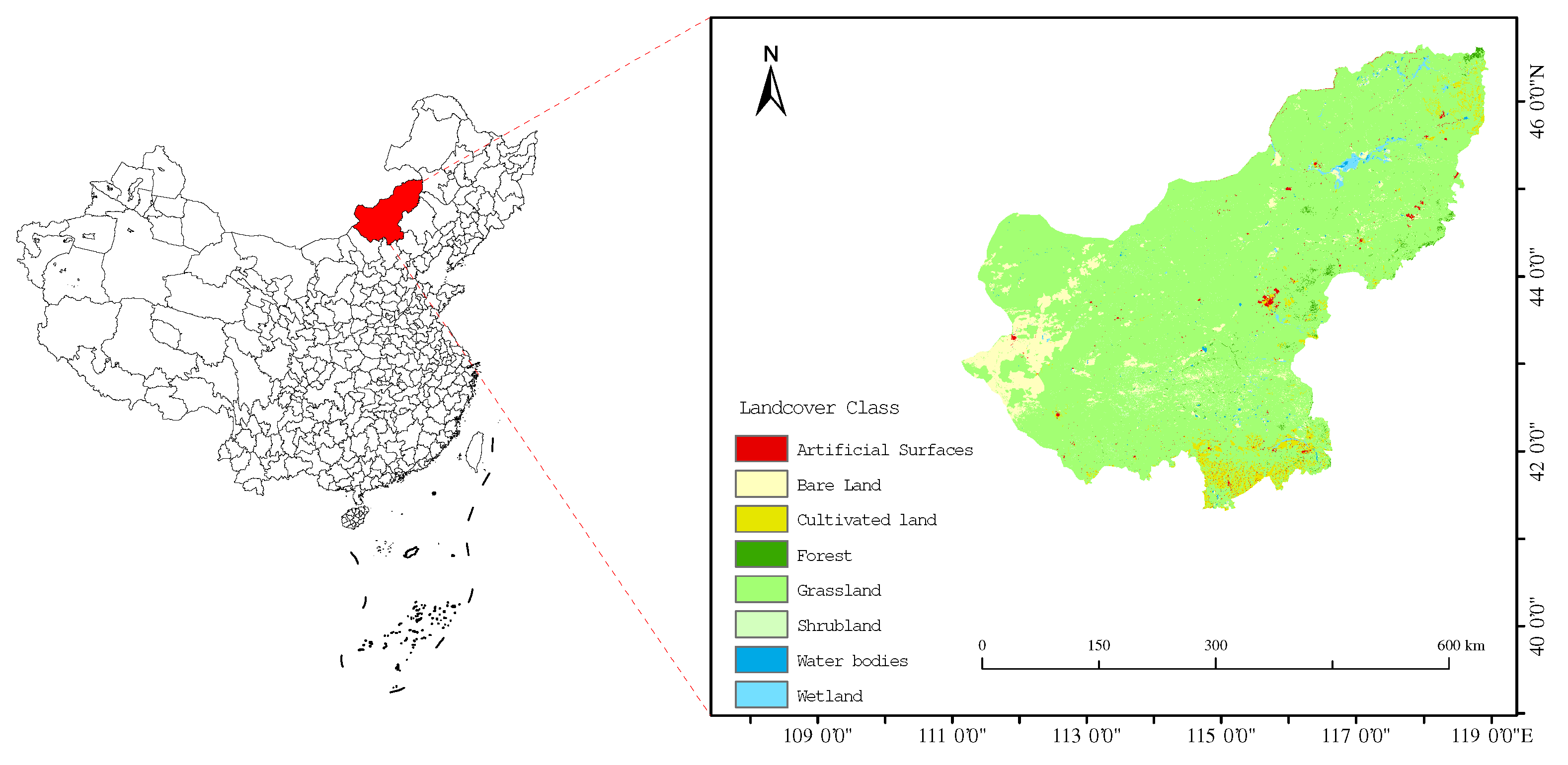
2.1. Data Sources

Located in the central part of the Inner Mongolia Autonomous Region and the southeastern edge of the Inner Mongolia Plateau, the Xilingol League has a semi-arid and arid continental monsoon climate in the middle temperate zone. It acts as a transitional region between the humid area in eastern China and the arid region in northwestern China, as well as the boundary between the agricultural and pastoral zones in northern China. The main body of the Xilingol League is a typical warm grassland area in northern China. To the east, there is the Daxinganling forest area, while to the south, it serves as an interlacing zone for agriculture and animal husbandry. Based on the land use type map of the Xilingol League in 2020 (Figure 1), it is evident that grassland dominates the region, encompassing a vast area across all banners and counties within the league. This grassland covers approximately 173,000 square kilometres, constituting roughly 86.3% of the region’s total land area. Therefore, analyzing and predicting precipitation in this region is crucial for studying vegetation growth and grazing strategies.

We use daily precipitation data from the “China_1km_prep_year” dataset [25] for the years from 2006–2019 and the GPM-IMERG dataset [26] from January 2021 to April 2023. Since the GPM-IMERG dataset has a spatial resolution of $10\mathrm{km}\times 10\mathrm{km}$, we utilized ArcGIS 10.8 software to convert its spatial resolution to $1\mathrm{km}\times 1\mathrm{km}$ to harmonize it with the data from prior years. The topic beyond this paper is to study grazing strategies in the Xilingol League. It also involves examining the growth of pasture grasses in the area, which is affected by factors such as precipitation, air temperature, and surface humidity. In addition to precipitation data, we introduced the annual mean temperature dataset, the annual NDVI dataset, and the global 1 km surface soil moisture dataset [27]. The annual mean temperature dataset is derived from the ERA5-Land dataset published by organizations such as the European Union and the European Centre for Medium-Range Weather Forecasts [28]; the annual NDVI dataset is obtained from the month-by-month NDVI raster data from the MOD13A3 dataset at https://search.earthdata.nasa.gov/search (accessed on 17 March 2023) and then obtained using the maximum synthesis method. For the research conducted in this paper, these datasets will aid us in identifying the specific regions where precipitation exhibits the highest correlation with the NDVI. These identified areas will serve as our focal regions for studying precipitation.

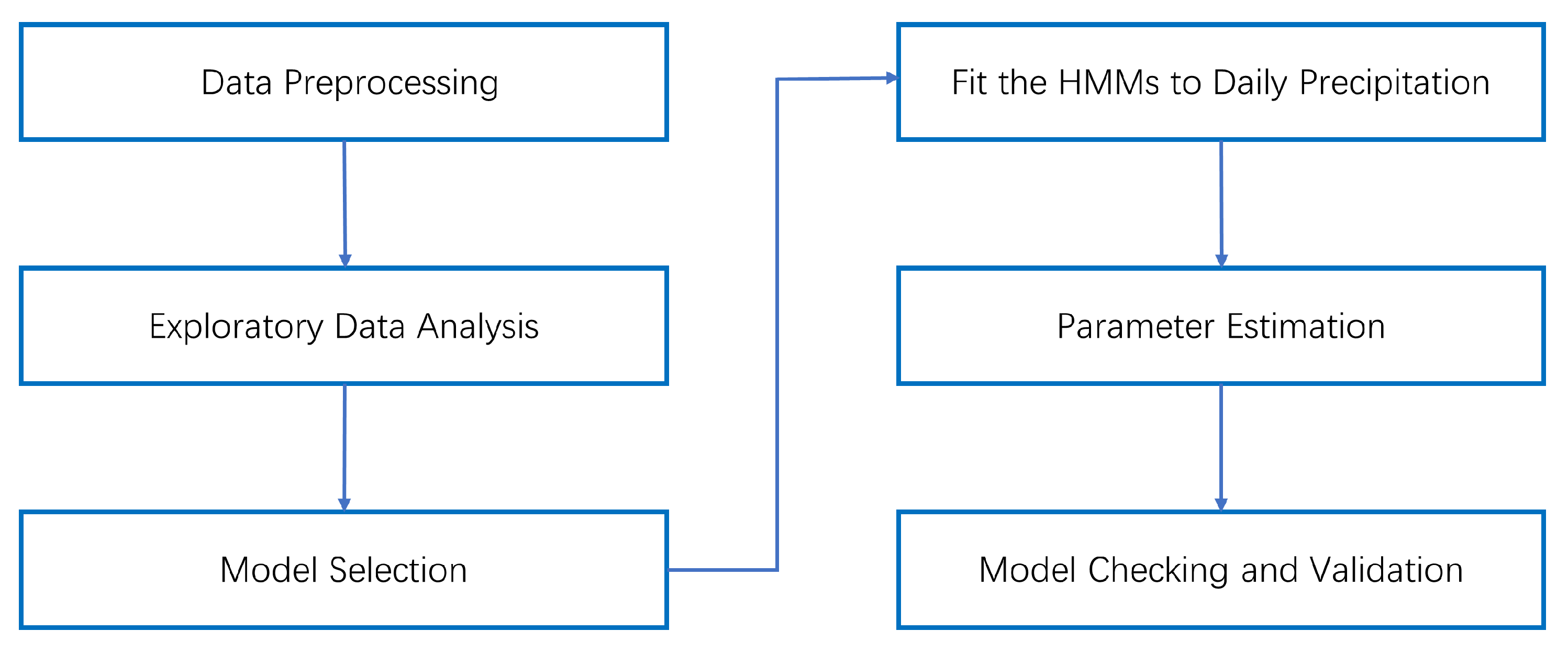
2.2. Methodology Workflow

This workflow summarizes the key steps in our study, from data collection to results interpretation, and illustrates the logical flow of our research process:

(1) We collected four kinds of raster datasets (Section 2.1) in TIFF format and cropped them to an appropriate size according to the administrative map of the Xilingol League. Then, we used ArcGIS 10.8 software to standardize the spatial resolution of all raster datasets so that they correspond point-to-point.

(2) We stacked the processed daily precipitation datasets (from 2006–2020) to create the annual precipitation dataset. Then, we conducted a correlation analysis on the annual precipitation dataset and the NDVI dataset (from 2006–2020). Subsequently, based on the four datasets, we performed partial correlation analysis with respect to the annual precipitation dataset and NDVI dataset. We selected regions where both the correlation and partial correlation of the two datasets are equal to or exceed 0.9 as the focal areas for our precipitation research. We will present the results of the data analysis in Section 3.2.1.

(3) Using randomly generated simulated precipitation datasets and Bayesian Information Criterion (BIC) scores, we determined the appropriate number of states and mixture components for fitting Hidden Markov Models (HMMs) to daily precipitation data. We will detail this process in Section 3.1.1.

(4) In the core of our HMMs, we established distribution models corresponding to three emission distributions: exponential distribution, gamma distribution, and a Pareto distribution model with a hierarchical structure. These models were used to fit the daily precipitation data. We will present the process of establishing the model in Section 2.3.

(5) We applied the three distribution models to three specific study areas selected from the Xilingol League, and we will perform parameter estimation based on the corresponding daily precipitation data (from 2006–2020). The parameter estimation methods used in this paper are the VBEM and SVB algorithms. We will present the detailed process of parameter estimation in Section 2.4.

(6) Finally, we conducted checks and validation of the model’s fitting and prediction capabilities through simulation experiments in Section 3.1 and empirical analysis in Section 3.2.

To provide a visual representation of our methodology, we have included the following workflow diagram (Figure 2):

2.3. The HMM for Precipitation

Consider a Hidden Markov Model for precipitation events. Suppose $y_{1:T}=\{y_1,\dots ,$$y_T\}$ is a precipitation time series with length $\mathrm{T}$ and $y_t\ge 0$. The series is generated by a set of potential hidden states $s_{1:T}=\left\{s_1,\dots ,s_t,\dots ,s_T\right\}$, where each state $s_t\in \{1,\dots ,K\}$. For each state j and daily precipitation data at G locations, we define indicator variables $l_{tjgm}$ that connect the hidden states to the emission distributions that generate precipitation such that: $l_{tjgm}{s}_{tj}=\mathbb{I}\left\{y_{tg}\mathrm{comes}\mathrm{from}\mathrm{the}{m}_{th}\mathrm{mixture}\mathrm{component}\mathrm{and}{s}_t=j\right\},$ with $g=1,\dots ,G$, and $m=0,1,\dots ,M$. The number of states $\left(K\right)$, locations $\left(G\right)$, and mixture components $(M+1)$ are assumed to be known. Since the weather state and mixing components are unique for any given day, $l_{tj}=\left(l_{tj0},l_{tj1},\dots ,l_{tjm}\right)$ is encoded as a one-hot vector and $l_{tj0}$ indicating no-precipitation events. For each state j and location g, $l_{tjg}=\left(l_{tjg0},\dots ,l_{tjgm}\right)$ follows a categorical distribution: $p\left(l_{tjg}\mid c_{jg},s_t=j\right)={\prod }_{m=0}^M{c}_{jgm}^{l_{tjgm}},$ where $p_j(·\mid ·)\equiv p\left(·\mid ·,s_t=j\right)$ coheres with the distribution for state $j,c_{jgm}$ are the mixture probabilities parameterizing $l_{tjg}$, with $c_{jgm}\ge 0$ for all m, and ${\sum }_{m=0}^M{c}_{jgm}=1$.

Let $x_{1:T}=\left\{x_1,\dots ,x_T\right\}$ be the precipitation time series in the observed data, where $X\mid \Lambda \sim Exp(\Lambda )$ and $\Lambda \sim Gamma(\gamma ,\eta )$. Then, the $m^{\mathrm{th}}$ mixture component (where $m>0$) from state j follows a Pareto distribution with scale ${\eta }_{jgm}$ and rate ${\gamma }_{jgm}$, i.e., $Y=X+\eta \sim Pareto(\eta ,\gamma )$; the distribution of an observation from state j is given by

$$\begin{array}{cc}\hfill p\left(y_{tg},l_{tjgm}\mid {\eta }_{jgm},{\gamma }_{jgm},c_{jgm},s_t=j\right)& =p\left(l_{tjgm}\mid c_{jgm},s_t=j\right)·p\left(y_{tg}\mid {\eta }_{jgm},{\gamma }_{jgm},l_{tjgm},s_t=j\right)\hfill \\ & =\prod _{m=0}^M{\left. [c_{jgm}\frac{{\gamma }_{jgm}{\eta }_{jgm}^{{\gamma }_{jgm}}}{y_{tg}^{{\gamma }_{jgm}+1}}\right]}^{l_{tjgm}}.\hfill \end{array}$$

The specific processes of establishing the exponential and gamma distributions as the emission distributions for generating precipitation can be respectively referred to the research works of Majumder et al. [22] and Bellone et al. [9].

2.4. VB Parameter Estimation for the HMM

The complete data likelihood in our HMM for precipitation is given by:

$$p(y,s,l\mid \Phi )=p(y,l\mid s,\Phi )·p(s\mid \Phi ),$$

where $p(s\mid \Phi )$ is the distribution of the states, which factorizes into the distribution of the initial state ${\pi }_1=p\left(s_1\right)$ and the distribution of the state transitions $p\left(s_{t+1}\mid s_t\right)$. For $j,k=1,\dots ,K,{\pi }_{1j}=Pr\left. [s_1=j\right]$ are the initial state probabilities and $a_{jk}=P\left. [s_{t+1}=k\mid s_t=j\right]$ are the state transition probabilities. $A=\left(\left(a_{jk}\right)\right)$ is the $K\times K$ state transition probabilities matrix, and $C=\left(\left(c_{jm}\right)\right)$ is the $K\times (M+1)$ matrix of mixture probabilities. $\mathrm{H}=\left(\left({\eta }_{jm}\right)\right)$ is a $K\times M$ matrix whose elements are the independently distributed rate parameters of the gamma distributions. Similarly, $\Gamma =\left(\left({\gamma }_{jm}\right)\right)$ is also a $K\times M$ matrix whose elements are the independently distributed scale parameters of the Pareto distributions, which are part of the semi-continuous emissions in each state. Taken together, $\Phi =\left({\pi }_1,A,C,\Gamma \right)$ parameterizes the HMM. We assign a prior on $\Phi$, which factorizes into a product over its components. That is, $p\left(\Phi \mid {\nu }^{\left(0\right)}\right)=p\left({\pi }_1\right)·p\left(A\right)·p\left(C\right)·p(\Gamma ),$ where ${\nu }^{\left(0\right)}$ are known hyperparameters. We assign independent Dirichlet priors to the rows of A and to the rows of C. Similarly, a Dirichlet prior is assigned to ${\pi }_1$. Note that a Dirichlet distribution is symmetric if the elements that make up its parameter vector are equal. The parameter vector’s concentration is defined as the sum of its elements. No prior information favoring one component over another is present when the Dirichlet distribution is symmetric. Finally, independent gamma priors are assigned to each element of $\mathrm{H}$ and $\Gamma$. That is,

$$\begin{array}{cc}\hfill p\left({\pi }_1\right)& =Dirichlet\left({\pi }_1\mid {\xi }^{\left(0\right)}\right),\hfill \\ \hfill p\left(A\right)& =\prod _{j=1}^{K}Dirichlet\left(a_j\mid {\alpha }_j^{\left(0\right)}\right),\hfill \\ \hfill p\left(C\right)& =\prod _{j=1}^K\prod _{g=1}^{G}Dirichlet\left(c_{jg}\mid {\zeta }_{jg}^{\left(0\right)}\right),\hfill \\ \hfill p\left(\mathrm{H}\right)& =\prod _{j=1}^K\prod _{g=1}^G\prod _{m=1}^{M}Gamma\left({\eta }_{jgm}\mid {\iota }_{jgm}^{\left(0\right)},{\delta }_{jgm}^{\left(0\right)}\right),\hfill \\ \hfill p(\Gamma )& =\prod _{j=1}^K\prod _{g=1}^G\prod _{m=1}^{M}Gamma\left({\gamma }_{jgm}\mid {\upsilon }_{jgm}^{\left(0\right)},{\omega }_{jgm}^{\left(0\right)}\right),\hfill \end{array}$$

where ${\xi }^{\left(0\right)}=\left({\xi }_1^{\left(0\right)},\dots {\xi }_K^{\left(0\right)}\right)$ denotes prior parameters of initial state probabilities ${\pi }_1$, ${\alpha }_j^{\left(0\right)}=\left({\alpha }_{j1}^{\left(0\right)},\dots ,{\alpha }_{jK}^{\left(0\right)}\right)$ denotes prior parameters of state transition probabilities $a_{jk}$, and ${\zeta }_{jg}^{\left(0\right)}=\left({\xi }_{jg0}^{\left(0\right)},\dots ,{\zeta }_{jgM}^{\left(0\right)}\right)$ denotes prior parameters of mixture probabilities $c_{jm}$. ${\gamma }_{jgm}$ and ${\eta }_{jgm}$ are the shape and rate parameters of the gamma distribution followed by $\Lambda$, respectively. When ${\gamma }_{jgm}$ is determined, we assign a gamma prior to ${\eta }_{jgm}$, with ${\iota }_{jgm}^{\left(0\right)}$ and ${\delta }_{jgm}^{\left(0\right)}$ as prior parameters. Similarly, ${\upsilon }_{jgm}^{\left(0\right)}$ and ${\omega }_{jgm}^{\left(0\right)}$ are the two parameters of the gamma prior corresponding to the shape parameter ${\gamma }_{jgm}$ in the Pareto distribution when the scale parameter ${\eta }_{jgm}$ is determined. The Pareto distribution here can be regarded as constructed by hierarchical exponential and gamma distributions, so that in the gamma distribution followed by $\Lambda$, the posterior ${\eta }_{jgm}^{\left(i_1\right)}$ of the rate parameter ${\eta }_{jgm}$ is the fixed value in the Pareto distribution when the scale parameter ${\eta }_{jgm}$ is determined.

The variational family $\mathrm{Q}$ for the posterior is restricted to distributions, which are separable in the following manner:

$$\begin{array}{cc}\hfill q(\Phi ,s,l)& =q_{\Phi }(\Phi )·q_{s,l}(s,l),\hfill \\ \hfill q_{\Phi }(\Phi )& =q\left({\pi }_1\right)·q\left(A\right)·q\left(C\right)·q(\Gamma ).\hfill \end{array}$$

The VBEM algorithm involves a cyclic process of updating the posterior for the model parameters, $q_{\Phi }(\Phi )$, and the posterior for the latent variables, $q_{s,l}(s,l)$. Algorithm 1 shows the complete VBEM algorithm. Posterior updates of $q_{\Phi }(\Phi )$ and $q_{s,r}(s,l)$ can be derived as closed-form expressions since our model is in the conjugate exponential family [17]. This approach is known as mean-field variational Bayes, and the optimization of the Evidence Lower Bound (ELBO) one parameter at a time, using all available data, is commonly referred to as Coordinate Ascent Variational Inference (CAVI) [15]. Details of the M-step (VBM) and E-step (VBE) for the VBEM algorithm can be found in Appendix A.

Algorithm 1 VBEM algorithm for HMMs

1: Initialize preparatory model parameters ${\Phi }_{\mathrm{p}}^{\left(0\right)}=\left({\pi }_1^{\left(0\right)},A^{\left(0\right)},C^{\left(0\right)},{\mathrm{H}}^{\left(0\right)}\right)$; 2: while (convergence criterion is not met) do 3:       Compute the latent variables $q_{tj}$ and $q_{jk}$ with forward–backward algorithm; 4:       Update the current estimate of preparatory model parameters $${\Phi }_{\mathrm{p}}^{\left(i_1\right)}=\left({\pi }_1^{\left(i_1\right)},A^{\left(i_1\right)},C^{\left(i_1\right)},{\mathrm{H}}^{\left(i_1\right)}\right);$$ 5: end while 6: Initialize model parameters ${\Phi }^{\left(0\right)}=\left({\pi }_1^{\left(i_1\right)},A^{\left(i_1\right)},C^{\left(i_1\right)},{\Gamma }^{\left(0\right)}\right)$ with ${\Phi }_{\mathrm{p}}^{\left(i_1\right)}$; 7: while (convergence criterion is not met) do 8:       Compute the latent variables $q_{tj}$ and $q_{jk}$ with forward–backward algorithm; 9:       Update the current estimate of preparatory model parameters $q_{\Phi }(\Phi )$; 10: end while

Stochastic Variational Bayes: Due to the necessity to compute posterior means for the parameters and latent variables at each iteration, which necessitates a pass over all of the data, the VBEM method might become constrained by the length of the data. The stochastic variational Bayes (SVB) method, which converts the VBEM algorithm into a stochastic gradient ascent algorithm for each parameter, is one of the stochastic optimization techniques that can speed up computing. SVB employs an unbiased estimate of the gradient at each iteration rather than computing gradients based on the complete dataset. Assuming exchangeable data for each year, we randomly sample the data based on stochastic gradient optimization. Afterwards, we replicate and fill the sampled data to enable iteration using minibatches of data, and these results will serve as the initial values for the complete time series iteration. Algorithm 2 gives the stochastic variational inference algorithm for HMMs. Specifically, the VBE step remains unchanged, while the VBM step involves stochastic gradient ascent with a step size of $\tau$. In the VBM step, we scale the expectations of the latent variables by a factor of N to encompass the entire dataset, and we outline the updating process of the hyperparameters in Appendix B.

Algorithm 2 Stochastic Variational Bayes for HMMs

1: Initialize preparatory model parameters ${\Phi }_{\mathrm{p}}^{\left(0\right)}=\left({\pi }_1^{\left(0\right)},A^{\left(0\right)},C^{\left(0\right)},{\mathrm{H}}^{\left(0\right)}\right)$; 2: Sample a subsequence ${\mathbf{x}}^D\subset \left\{x_1,\dots ,x_T\right\}$, where $D<T$; 3: while (convergence criterion is not met) do 4:       Set the step-size schedule ${\tau }_{i_1}$ appropriately; 5:       Compute intermediate preparatory model parameters ${\widehat{\Phi }}_{\mathrm{p}}$; 6:       Update the current estimate of preparatory model parameters $${\Phi }_{\mathrm{p}}^{\left(i_1^{*}\right)}=\left(1-{\tau }_{i_1^{*}}\right){\Phi }_{\mathrm{p}}^{(i_1^{*}-1)}+{\tau }_{i_1^{*}}·{\widehat{\Phi }}_{\mathrm{p}};$$ 7: end while 8: Initialize model parameters ${\Phi }^{\left(0\right)}=\left({\pi }_1^{\left(i_1^{*}\right)},A^{\left(i_1^{*}\right)},C^{\left(i_1^{*}\right)},{\Gamma }^{\left(0\right)}\right)$ with ${\Phi }_{\mathrm{p}}^{\left(i_1^{*}\right)}$; 9: while (convergence criterion is not met) do 10:       Set the step-size schedule ${\tau }_i$ appropriately; 11:       Compute intermediate preparatory model parameters $\widehat{\Phi }$; 12:       Update the current estimate of preparatory model parameters $${\Phi }^{\left(i\right)}=\left(1-{\tau }_i\right){\Phi }^{(i-1)}+{\tau }_i·\widehat{\Phi };$$ 13: end while

Assessing Convergence: We compute and track the ELBO at each iteration to assess the convergence of the VBEM algorithm. The ELBO for our model can be expressed as:

$$ELBO\left(q\right)={\mathbb{E}}_{q(s,l)}logp(y,s,l)+{\mathbb{E}}_{q(\Phi )}logp(\Phi )+H\left(q(s,l)\right)-{\mathbb{E}}_{q(\Phi )}logq(\Phi ),$$

where $H\left(q\right(s,l\left)\right)$ is the entropy of the variational posterior distribution over the latent variables. This simplifies to [18,19]:

$$\begin{array}{cc}\hfill ELBO\left(q\right)=logq(y\mid \tilde{\Phi })& -KL\left(q\left({\pi }_1\right)\parallel p\left({\pi }_1\right)\right)-KL(q\left(A\right)\parallel p\left(A\right))\hfill \\ & -KL\left(q\right(C)\parallel p(C\left)\right)-KL\left(q\right(\Gamma )\parallel p(\Gamma \left)\right),\hfill \end{array}$$

where $logq(y\mid \tilde{\Phi })$ is calculated using Equation (A3) in the forward algorithm of Appendix C, and the analytic formula for $\mathrm{KL}$ divergence is listed in Appendix D. We employ this relationship to calculate the ELBO at each iteration, and we declare convergence once the change in ELBO drops below a predetermined threshold.

3. Results

3.1. Simulation Study

In this paper, we use randomly generated precipitation data with a time length of 1380 as the original data. If the daily precipitation is sorted from largest to smallest, the range of the first six precipitation amounts is [48.19, 101.15] in mm, and the range of the remaining precipitation amounts is within 26.64 mm. Setting up the precipitation data in this way not only allows for assessing the average level of precipitation generated by the precipitation generator but also the accuracy of its generation of the heavy or torrential precipitation fraction.

Table 1. The correspondence between precipitation levels and daily precipitation.

Precipitation Level	Daily Precipitation Amounts Ranges
Light Precipitation	<10 mm
Moderate Precipitation	[10 mm, 25 mm]
Heavy Precipitation	[25 mm, 50 mm]
Torrential Precipitation	[50 mm, 100 mm]
Heavy Storms	[100 mm, 200 mm]
Torrential Storms	>200 mm

shows the correspondence between precipitation levels and daily precipitation, with reference to the classification of rainfall levels by the China Meteorological Administration (CMA). Due to the random nature of the precipitation generated by the stochastic precipitation generator, we generated 100 datasets based on the results of the variational posterior, and the following evaluation metrics are taken from the average of the evaluation results of the 100 datasets.

3.1.1. BIC Scores for Daily Precipitation

The model selection problem seeks an optimal balance between model complexity and the model’s ability to describe the datasets. Bayesian information criterion (BIC), introduced by Schwarz, is derived to serve as an asymptotic approximation to a transformation of the Bayesian posterior probability of a candidate model [29]. BIC is a statistical method for choosing the most suitable model from a finite set of models. Its widespread use is attributed to its computational simplicity and strong performance across various modeling frameworks, even in cases where prior distributions are difficult to define in Bayesian applications. In situations with large sample sizes, the model preferred by BIC ideally aligns with the candidate model that is a posteriori most likely, meaning it is the model that the data at hand makes most plausible. The definition of BIC or BIC scores for the models is available in Appendix E.

The Bayesian Information Criterion (BIC) scores of the models are used to measure the model goodness of fit, where a lower BIC score indicates a better model fit. However, Bellone [30] has previously demonstrated that the theoretical underpinnings of the most common likelihood-based techniques are untenable in a sequential selection setting, such as the BIC used in this paper, and should not be used as the sole criterion for model selection. However, its results can also be used as a reference for model selection and cross-sectional analysis with other metrics.

Table 2. BIC scores for daily precipitation in HMMs.

Number of Hidden States	Exponential Distribution		Gamma Distribution		Pareto Distribution
	C = 3	C = 4	C = 3	C = 4	C = 3	C = 4
3	6124.92	6118.54	6490.61	6503.58	5679.57	5680.50
4	6131.62	6120.89	6465.26	6519.02	5711.61	5700.50
5	6624.81	6493.07	6617.57	6626.71	5690.45	5691.82
6	6595.85	6472.56	6669.12	6619.91	5695.55	5692.39

presents the BIC scores obtained when utilizing the exponential, gamma, and Pareto distributions as models for generating positive precipitation within HMMs. We also compared the different numbers of states and mixture components for each distribution to find the optimal state transfer matrix and mix probability matrix of the fitting model through simulation.

3.1.2. RMSE for Heavy Precipitation Weather

Considering the variability of precipitation in different regions in the actual problem, we choose the precipitation amount ranked in the top 10 to evaluate extreme weather precipitation. The evaluation index is the Root Mean Squared Error (RMSE). Similar to the BIC table, we replace its value with the RMSEs of the 10 extreme weather precipitation amounts.

Table 3. RMSEs for heavy precipitation weather in HMMs.

Number of Hidden States	Exponential Distribution		Gamma Distribution		Pareto Distribution
	C = 3	C = 4	C = 3	C = 4	C = 3	C = 4
3	44.94	44.79	67.01	68.61	21.70	21.74
4	45.05	44.36	64.09	68.79	25.30	23.94
5	82.85	73.09	72.80	76.05	3.15	4.84
6	80.58	71.87	78.19	80.80	4.45	3.11

shows the RMSEs of the 10 extreme weather precipitation amounts for the three positive precipitation distribution models. The result indicates that the Pareto distribution consistently exhibits the lowest RMSE across various combinations of hidden states and mixture components. Unlike the exponential and gamma distributions, the Pareto distribution is closer to the true value (where the true value refers to the randomly generated original precipitation data with a time duration of 1380) for high precipitation with the number of hidden states of 5 and 6, while the high precipitation generated by the exponential and gamma distributions is further away from the true value. The result indicates that for model fitting of high precipitation levels, the exponential and gamma distributions are more suitable for model fitting with 3-state and 4-state, while the Pareto distribution is more suitable for model fitting with 5-state and 6-state.

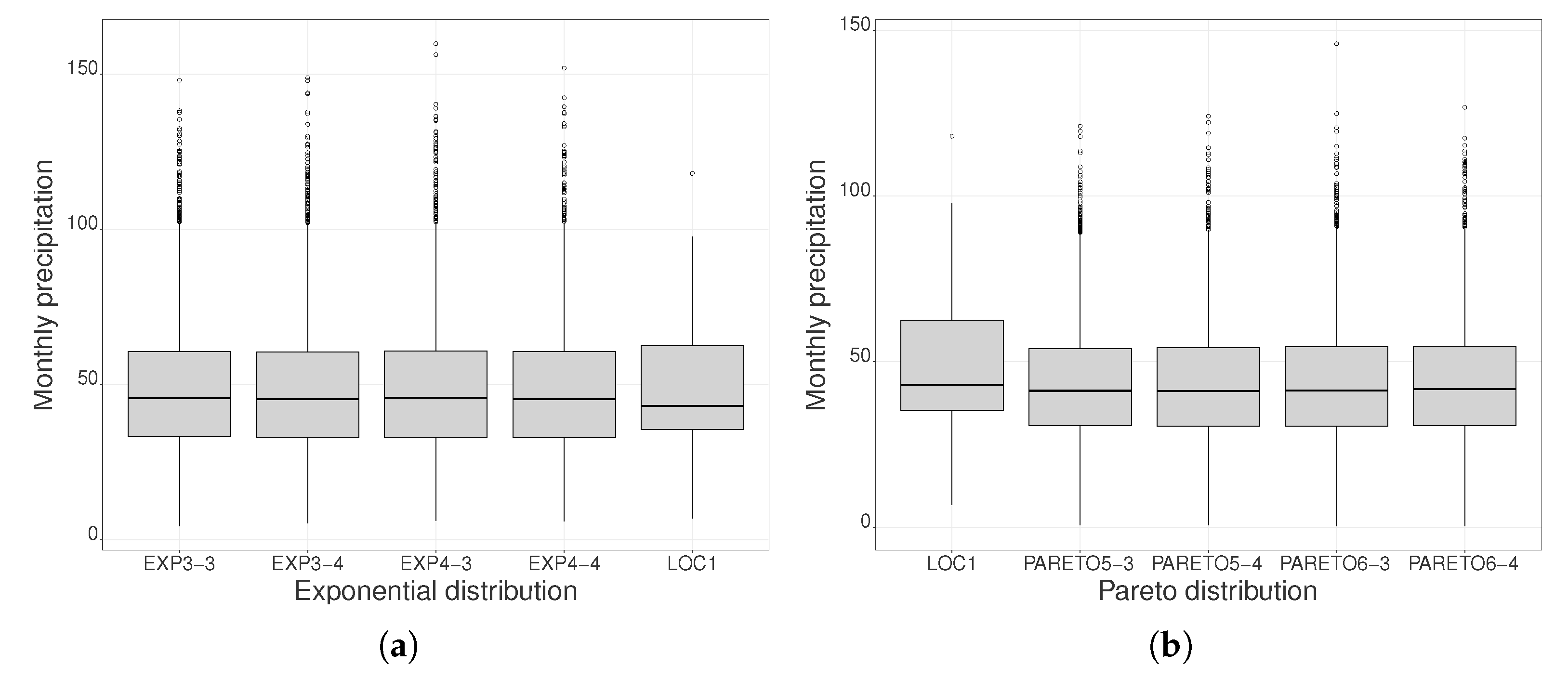
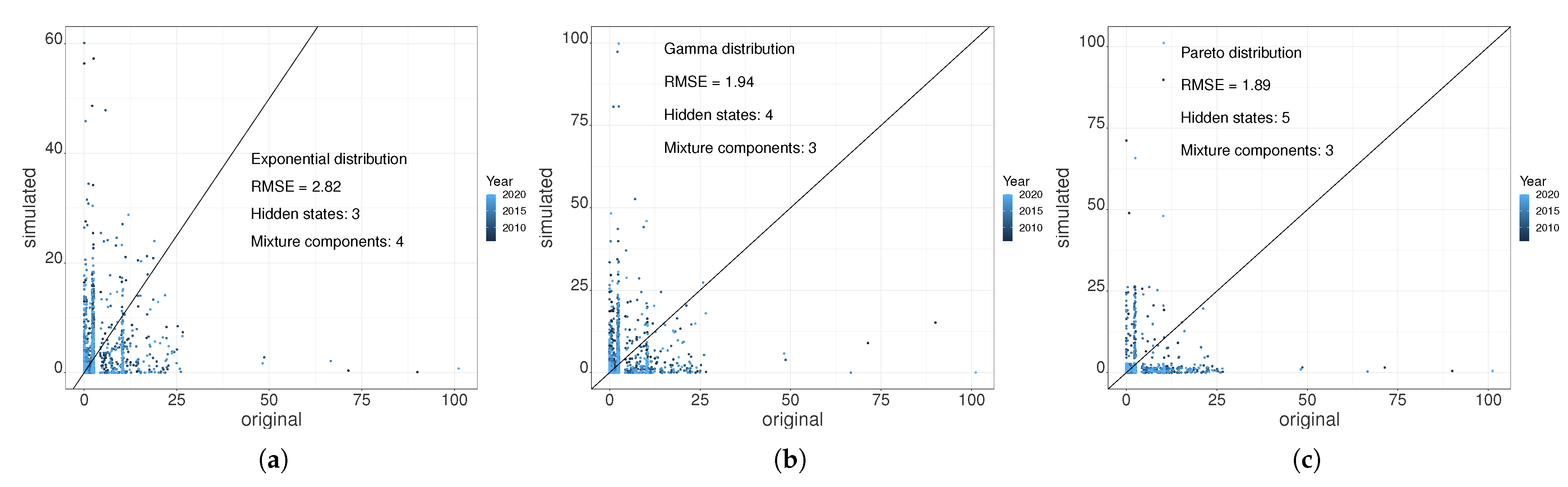
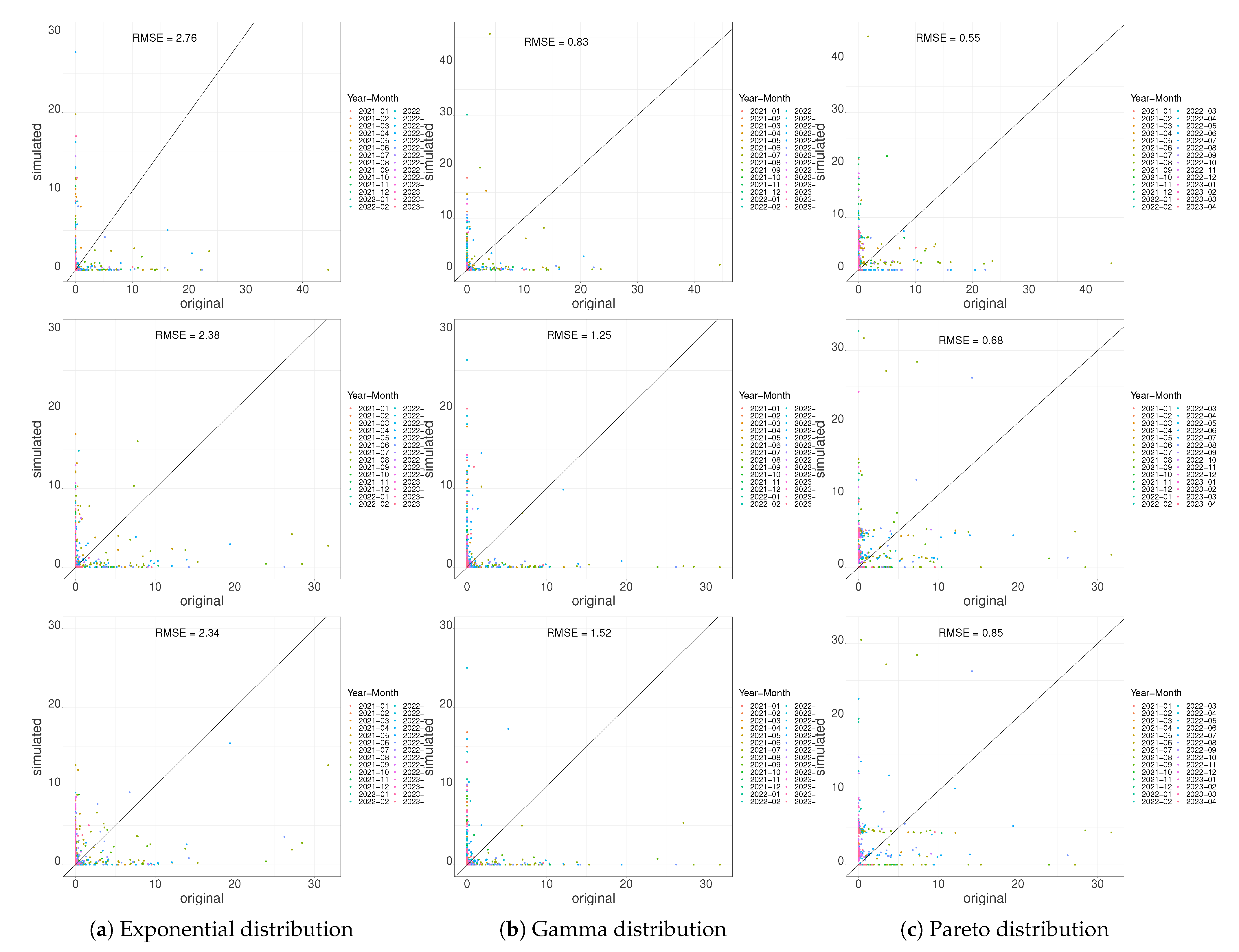
3.1.3. Scatter Plot Regression of Daily Precipitation

Based on the evaluation results of both BIC and RMSE metrics, we select the appropriate number of states and mixture components for the three positive precipitation distributions to serve as the kernel of the random precipitation generator in this paper. We observe the regression fit of the simulated precipitation data and the precipitation data generated by the stochastic precipitation generator by plotting the scatter plot of the two data types. The number of hidden states and mixture components for HMMs considers the BIC score and the RMSE of high precipitation amounts.

Note that the scatter plot is labeled with the RMSE of all data with a time step of 1380, reflecting the overall deviation of the simulated precipitation data generated by the stochastic precipitation generator from the original precipitation data. As shown in Figure 3, the Pareto distribution model has the lowest RMSE, indicating the best fit for the overall precipitation. The scatter plot also illustrates that almost all the precipitation generated by the Pareto distribution model is concentrated within 26.64 mm, aligning closely with the true value. In contrast, a significant portion of the precipitation generated by the gamma distribution model falls in the range of 25–45 mm, showing a more significant deviation from the true value, which is uncontrollable. Moreover, the exponential distribution model not only shares the same limitations as the gamma distribution model in fitting heavy precipitation but also performs poorly in representing torrential precipitation. The Pareto distribution model effectively addresses these shortcomings, offering controllable precipitation generation across all levels.

3.2. Analysis of Daily Precipitation in the Xilingol League

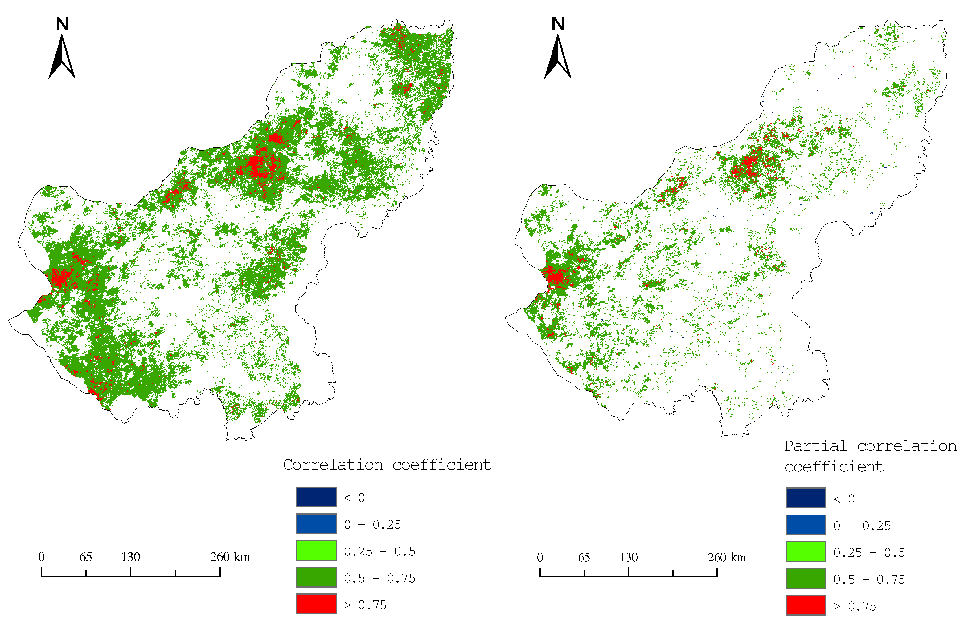
3.2.1. Annual Precipitation and NDVI Correlation Analysis

In this paper, we conducted correlation analysis and bias correlation analysis between precipitation and NDVI in the Xilingol League. The data used are annual precipitation raster data, annual NDVI raster data, annual average temperature raster data, and annual average surface soil moisture raster data for the Xilingol League region from 2006 to 2020.

From the correlation graph of NDVI and annual precipitation that passed the significance test (Figure 4), we observe the following patterns: certain concentrated areas, primarily in the north and west, with a few in the northeast and southwest, exhibit a notably strong positive correlation (r > 0.75) between NDVI and annual precipitation, covering approximately 2.2% of the region; approximately 37.1% of the areas display a significant positive correlation (r > 0.5) between NDVI and annual precipitation; there are minimal instances of significant negative correlation (r > 0.5) between NDVI and annual precipitation. In summary, around 37.1% of the areas show a significant positive correlation (r > 0.5) between NDVI and annual precipitation, while there are hardly any areas with a significant negative correlation between NDVI and annual precipitation. From the bias correlation graph of NDVI and annual precipitation that passed the t-test (Figure 4), we observe the following: the number of areas with a significant correlation between NDVI and annual precipitation, as determined by the t-test, has significantly reduced, accounting for 13.8%; the number of areas with a significant strong positive correlation has also decreased to some extent, accounting for 1.2%. Furthermore, in this paper, we will focus on the regions with strong positive correlation or partial correlation that have passed the significance test or t-test to predict future precipitation patterns.

The final selection of raster point information to be analyzed and predicted for precipitation is shown in

Table 4. The regions with a significant, strong positive correlation and partial correlation between NDVI and annual precipitation that have passed the significance test and t-test, respectively.

Location	Longitude	Latitude	Correlation Coefficient	Partial Correlation Coefficient
1	${114}^{\circ }{21}^{\prime }$ E	${44}^{\circ }{51}^{\prime }$ N	0.90	0.90
2	${115}^{\circ }{52}^{\prime }$ E	${44}^{\circ }{59}^{\prime }$ N	0.91	0.93
3	${115}^{\circ }{54}^{\prime }$ E	${44}^{\circ }{59}^{\prime }$ N	0.93	0.90

.

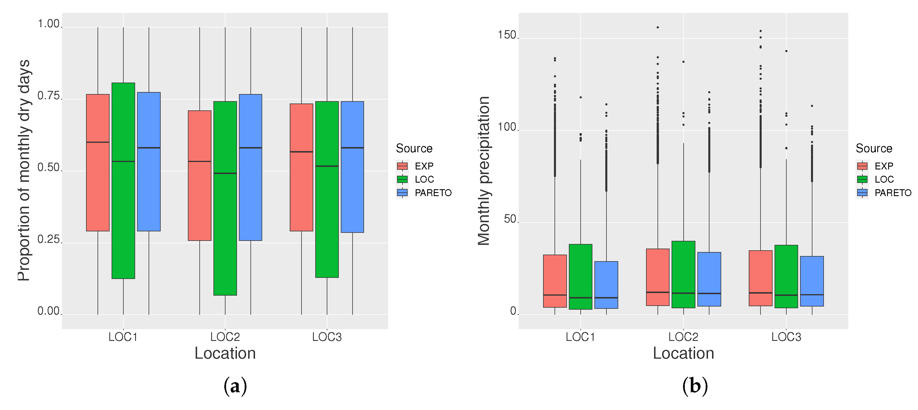
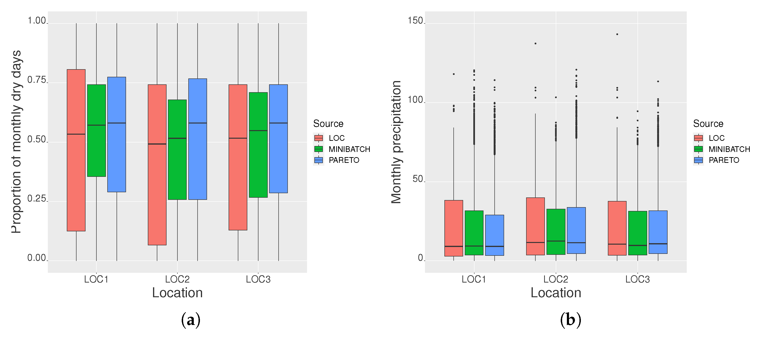
3.2.2. Seasonal Precipitation Sequences

In this paper, we analyze seasonal precipitation series generated by the exponential and Pareto distributions using box plots compared to the actual observation values. Based on our simulation results, we choose 3-state and 4-state models for the exponential distribution and 5-state and 6-state models for the Pareto distribution. It is worth noting that the results we present in this paper rely on precipitation data obtained from 100 groups of simulations, so encountering more outlier points is to be expected. The following figures illustrate precipitation patterns at the location ${114}^{\circ }{21}^{\prime }$ E, ${44}^{\circ }{51}^{\prime }$ N as an example.

Figure 5a shows that the upper and lower quartiles of monthly precipitation totals are lower than the actual observation value, and the median and maximum values are higher than the actual observation value for each condition of the exponential distribution model. In general, the upper quartiles, lower quartiles, and median are closer to the actual observation value. Among them, the maximum value of monthly precipitation under the 4-state and 3-component conditions is closer to the actual observation value than the other conditions. Therefore, the precipitation series generated under the 4-state and 3-component conditions is the most similar to the actual observation value. Figure 5b shows that the Pareto distribution model has less than the actual observation value for each indicator of total monthly precipitation for all conditions. On the whole, the precipitation series generated under the 6-state and 4-component conditions are more similar to the actual observation values.

Figure 6a shows that the simulations of the model constructed by both distributions for the proportion of seasonal monthly dry days are significantly different from the actual observation values. Figure 6b shows that the upper and lower quartiles of the precipitation series of the exponential distribution at position 1 are closer to the actual observation value, and the median of the precipitation series of the Pareto distribution is closer to the actual observation value; the upper and lower quartiles of the precipitation series of the Pareto distribution at locations 2 and 3 are closer to the actual observation value, and the median of the precipitation series of the exponential distribution is closer to the actual observation value. In summary, the seasonal monthly precipitation totals generated by the two distributions have mutual advantages and disadvantages in terms of upper and lower quartiles and median indicators. The exponential distribution model performs better in terms of minimum values, and the Pareto distribution model performs better in terms of the number and range of outlier points. In contrast, the performance on the number and range of anomaly points is the indicator we are more interested in, i.e., the generation of heavy precipitation under extreme weather conditions.

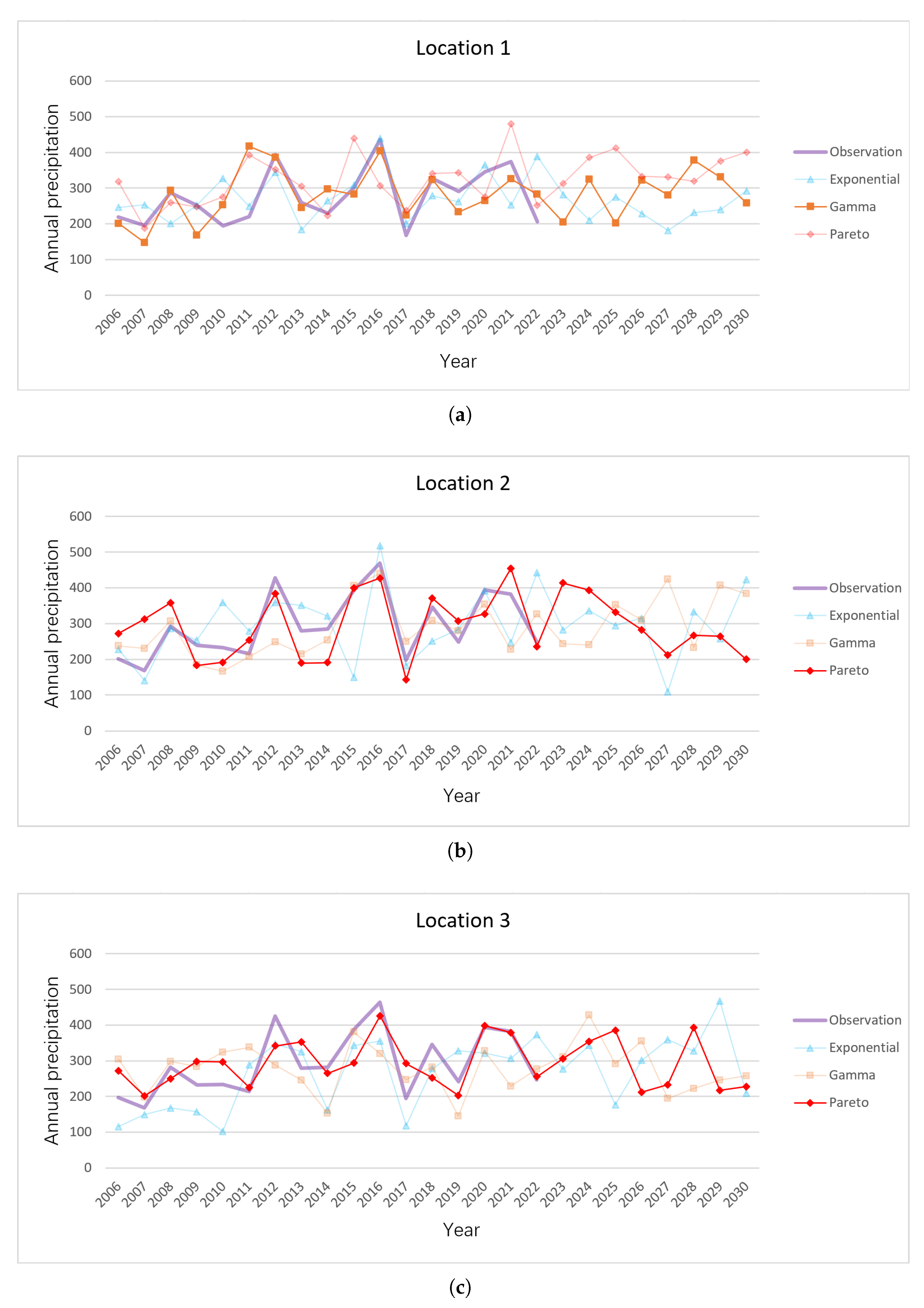
3.2.3. Annual Precipitation Sequence

Figure 7a shows that the two distributions perform better for the generation of annual precipitation series compared to seasonal precipitation series in terms of the proportion of monthly dry days. Among them, the upper quartile of the Pareto distribution model is closer to the actual observation value at all three positions, and from the comparison of the medians, the Pareto distribution model is closer to the actual observation value at position 1, and the exponential distribution model is closer to the actual observation value at positions 2 and 3. Figure 7b demonstrates that, at all locations, the upper quartile of the exponential distribution model aligns more closely with the actual observation value, while the median and lower quartile of the Pareto distribution model are in better agreement with the actual observation value. Additionally, the Pareto distribution model displays significantly fewer outliers, and the range of its values better matches the actual observation values compared to the exponential distribution model.

On the whole, for the time series of annual precipitation, the Pareto distribution model fits better than the exponential distribution model for the average level of precipitation as well as the intense precipitation. To improve the iteration rate of parameter estimation, we introduce the SVB method. In this paper, stochastic gradient optimization with step size ${\tau }_i={(1+i)}^{-0.9}$ is run for the first 500 iterations, followed by 200 iterations using the CAVI method on all data to ensure convergence. The initial value of the CAVI method before iteration is the value of the stochastic gradient optimization with 500 iterations, which theoretically runs about 15 times faster than the CAVI method (this multiple is equal to the number of years of precipitation data), so it can significantly increase the rate of parameter estimation. Figure 8 presents box plots of the proportion of dry days and precipitation generated from the parameters estimated using the SVB method and the CAVI method in the Pareto distribution model. Figure 8 reveals that the parameters estimated through iteration with stochastic gradient optimization on mini-batches of data have minimal impact on the final generated results and, in some cases, even yield better performance for certain metrics at specific locations. Therefore, the introduction of the SVB method is necessary when it is necessary to generate precipitation sequences for a large number of location points.

We used daily precipitation data from 2006 to 2020 to train our models. The previous work validated the suitability of the Pareto distribution model through two indicators: monthly precipitation and the ratio of sunny days from 2006 to 2020. The theoretical basis for this approach was developed, drawing from the research conducted by Majumder et al. [22]. Next, we assessed the performance of each distribution model in predicting precipitation using observed data from January 2021 to April 2023. The evaluation metrics for model prediction performance include Root Mean Square Error (RMSE) for simulated daily precipitation, monthly precipitation, annual precipitation, and the actual ground truth data. We generated 100 sets of daily precipitation sequences for the years 2006 to 2030 using each of the three models. By calculating the RMSE for annual precipitation from 2006 to 2020, we ultimately selected the precipitation sequence corresponding to the minimum RMSE out of the 100 sets as the optimal result for each model.

From

Table 5. RMSEs of precipitation in three time dimensions of day, month, and year from January 2021 to April 2023.

Location	Distribution	Daily Precipitation	Monthly Precipitation	Annual Precipitation
1	Exponential	2.76	35.66	154.59
1	Gamma	0.83	26.82	63.63
1	Pareto	0.55	35.21	81.64
2	Exponential	2.38	46.38	167.72
2	Gamma	1.25	36.54	123.8
2	Pareto	0.68	36.14	110.97
3	Exponential	2.34	39.82	68.9
3	Gamma	1.52	34.32	50.95
3	Pareto	0.85	32.72	6.64

, we observe that the gamma distribution model exhibits the lowest RMSE values for monthly and annual precipitation at location 1, but it does not significantly outperform the Pareto distribution model. Overall, the Pareto distribution model demonstrates a clear advantage in predicting precipitation across the three time dimensions of year, month, and day. The best prediction is achieved for annual precipitation at location 3. In contrast, the exponential distribution model performs the worst, particularly in predicting annual precipitation at location 1 and monthly precipitation at location 2. Figure 9 illustrates the fitting of daily precipitation by different distribution models at the three locations. It is evident that the Pareto distribution model outperforms other distribution models across all three locations. The exponential distribution model exhibits the poorest overall performance (reflected in the RMSE values for daily precipitation in Table 5), particularly in predicting daily precipitation exceeding 20 mm. The gamma distribution model shows less stable performance in predicting daily precipitation exceeding 20 mm, which deviates from the simulation results presented in Section 3.1.3, indicating lower generalization ability of the gamma distribution model for predicting daily precipitation.

It is important to note that Table 5 shows the Pareto distribution has the lowest RMSE values for daily precipitation, while the RMSE values for monthly and annual precipitation may not be the lowest. This difference is due to our calculation of RMSE for daily precipitation based on sorted daily precipitation data. Therefore, the RMSE values for daily precipitation do not necessarily reflect the model’s predictive performance in the other two time dimensions. However, to accurately display the corresponding dates for daily precipitation, the data visualized on the scatter plot (Figure 9) has not undergone sorting. In addition, based on the fitting of regression lines to precipitation data points in Figure 9: for days with relatively high daily precipitation (exceeding 20 mm), simulated precipitation data and actual observed data share similar colors, indicating that they belong to the same month or adjacent months. However, for data points with values that are close to each other, their distances from the regression line are relatively far, suggesting that the simulated precipitation data corresponding to the actual observed data did not occur on the same day.

3.2.4. Analysis of Annual Precipitation Trends

We compiled the annual precipitation data for 2006–2030 at the three locations in the Xilingol League. Figure 10 presents the annual precipitation computed based on actual historical daily data from 2006 to 2022 and the annual precipitation calculated from daily precipitation sequences simulated by the three distribution models from 2006 to 2030. The selection of the predictive distribution models relies on the RMSE for annual precipitation in 2021 and 2022. At location 1, the gamma distribution model corresponds to the lowest RMSE, while at locations 2 and 3, the Pareto distribution model exhibits the lowest RMSE. Therefore, the primary choice for predicting annual precipitation for the years 2023 to 2030 is the distribution model corresponding to the minimum RMSE.

Based on the predictive results, it is clear that annual precipitation at all three locations falls within the range of approximately 200 mm to 400 mm. According to the primary predictive model at location 2 (Pareto distribution model), annual precipitation for the years 2026 to 2030 consistently falls below 300 mm, suggesting the need for precautions against the potential impact of reduced natural precipitation on grass growth and adjustments in grazing strategies. Additionally, at location 2, the exponential distribution model generates an unusual prediction of 109.51 mm for the year 2027. This prediction somewhat indicates the potential for reduced natural precipitation. Furthermore, the exponential distribution model predicts a historical peak (467.86 mm) in annual precipitation at location 3 in the year 2029, indicating the necessity of precautions against the potential impact of heavy precipitation on grass growth and adjustments in grazing strategies. In contrast, the predictive results for location 1 appear relatively stable, suggesting a lesser need for additional control measures.

For those interested in analyzing pasture growth and obtaining more ecological insights through seasonal variations in precipitation, they can compile monthly precipitation data and frequency statistics based on the available daily precipitation data.

4. Conclusions

In the simulation experiments section of this study, the researchers employed the Hidden Markov Model (HMM) framework, incorporating three emission distributions: the exponential distribution, gamma distribution, and Pareto distribution. They used Bayesian Information Criterion (BIC) to determine the appropriate order for the state transition matrix and the mixture probability matrix required for accurately generating daily precipitation sequences. Specifically, for the exponential and gamma distributions, state transition matrices of orders 3 and 4 were found suitable for model fitting. In the case of the Pareto distribution, we chose state transition matrices of orders 5 and 6 for model fitting. In the empirical research section, we chose locations within the Xilingol League where annual precipitation significantly affects NDVI as our research subjects. Building on the work of Majumder et al. [22], we first validated the suitability of the Pareto distribution model for fitting daily precipitation using rainy-season daily precipitation data from 2006 to 2020, which involved calculating monthly precipitation and dry days ratios. Subsequently, we further validated the Pareto distribution model’s suitability for fitting daily precipitation using full-year daily precipitation data, calculating monthly precipitation and dry days ratios.

Finally, we evaluated the predictive performance of the Stochastic Precipitation Generator (SPG) using observed precipitation data from January 2021 to April 2023. Our findings indicate that, compared to the other two distributions, the Pareto distribution exhibited relatively better overall predictive performance across daily, monthly, and annual time dimensions. However, as analyzed from the results in Figure 9, none of the emission distributions could precisely allocate precipitation amounts to each individual day. Even the optimal Pareto distribution model could only provide a rough indication of when heavy or torrential precipitation might occur within a given month. Despite this limitation, when it comes to predicting extreme precipitation events or monthly and annual precipitation, Hidden Markov Models (HMMs) with Pareto distribution as the emission distribution may be the best candidates for Statistical Precipitation Generators (SPGs) in the Xilingol League. Nevertheless, this conclusion should be further validated at other locations.

5. Discussion

In Section 3.2 of this paper, we employed Hidden Markov Models (HMMs) to fit daily precipitation data in the Xilingol League. Building upon the theoretical foundations laid out by Bellone et al. and Majumder et al., we used three different distributions to simulate the generation of positive daily precipitation. In comparison to prior work, we extended the theoretical derivation process for the application of the hierarchical Pareto distribution model and conducted parameter estimation using the Variational Bayesian method. The rationality of this distribution model’s parameter estimation algorithm and its applicability in fitting daily precipitation were validated both in the simulation study (Section 3.1) and empirical research (Section 3.2). During the process of model and algorithm validation, we introduced continuous precipitation data for the entire year to further ascertain the applicability of the Stochastic Precipitation Generator (SPG). Additionally, this paper explored the performance of SPG in practical forecasting, compared the actual effects of the three distribution models in predicting precipitation across daily, monthly, and annual timeframes, and drew corresponding conclusions (Section 4). These findings have practical implications for guiding future grazing strategies in the Xilingol League region. In summary, we have comprehensively demonstrated the performance of the Stochastic Precipitation Generator (SPG) in generating random precipitation from both a model innovation and application expansion perspective, providing a more comprehensive view compared to previous research efforts.

Our research operates under the presumption of temporal stationarity, which involves considering two types of stationarity. Within a year’s data, stationarity is the first. This is tackled by focusing solely on seasonal data, an approach that aligns with previous studies. Moreover, we assume that the states remain constant from one year to the next, allowing for the interchangeability of precipitation data for the same month across different years. Stochastic optimization has made use of this premise. This assumption appears reasonable, as it is unlikely that the fundamental climate conditions have undergone substantial changes over the 15-year period covered by our data. However, a more thorough investigation is required to confirm this assumption for long periods during which climatic patterns may undergo alterations. From the research results presented in this paper, it is evident that SPG still exhibits certain limitations. Figure 6 and Figure 7 demonstrate that the HMMs, with parameters estimated using the VBEM algorithm, closely simulate the percentage of monthly dry days in the annual data’s time dimension compared to the historical data, especially when contrasted with the time dimension of the rainy season data. The conclusion also implies that the SPG’s ability to simulate precipitation frequency during the rainy season or non-continuous precipitation frequency is not ideal. Furthermore, as discussed in Figure 9, it is evident that the daily precipitation data generated by SPG cannot accurately correspond to specific dates. In other words, the precipitation sequences generated by SPG cannot serve as daily weather forecasts. This assumption is logical since precise daily rainfall predictions require real-time synchronization of various meteorological factors.

Future precipitation modeling efforts will emphasize explicitly incorporating spatial dependencies by increasing the emission distribution using copula functions. While existing models capture the spatial patterns in the data to some extent, parameterizing the dependence will help identify the state or domain where it exerts the most substantial influence. It is especially crucial for precipitation modeling due to its less smooth spatial distribution compared to temperature. Majumder et al. [31] used copula to estimate spatial correlations in HMMs, but this was conducted within the framework of maximum likelihood estimation using the Baum–Welch algorithm rather than in a Bayesian context. We would also like to use the reduced climate model output as a covariate of the model, as Robertson et al. [6] did. This method has two advantages—it would allow us to tune its behavior, and we would also be able to specify a more complex non-flush HMM (NHMM) in which the Markov chain parameters can vary according to month or even season [22,32]. However, it is essential to note that NHMM introduces additional computational complexity. The transition matrix parameters tend to be associated with covariates via logistic or probit link functions, and the final model may no longer belong to the family of covariate indices. From the perspective of the practical problem under study, we would like to achieve multivariate time series prediction, i.e., to study the growth of forage-based on multi-scale precipitation data, multiple meteorological factors and grazing strategies in different regions of the Xilingol League, and thus be able to propose reasonable scenarios for future grazing strategies in the region. We may use background knowledge such as Long Short-Term Memory (LSTM) networks and transformer-based modeling frameworks in deep learning.

References

1. Wilks, D.S. Interannual variability and extreme-value characteristics of several stochastic daily precipitation models. Agric. For. Meteorol. 1999, 93, 153–169. [Google Scholar] [CrossRef]
2. Kou, X.; Ge, J.; Wang, Y.; Zhang, C. Validation of the weather generator CLIGEN with daily precipitation data from the Loess Plateau, China. J. Hydrol. 2007, 347, 347–357. [Google Scholar] [CrossRef]
3. Wilks, D.S. Multisite generalization of a daily stochastic precipitation generation model. J. Hydrol. 1998, 210, 178–191. [Google Scholar] [CrossRef]
4. Rabiner, L.R. A tutorial on hidden Markov models and selected applications in speech recognition. Proc. IEEE 1989, 77, 257–286. [Google Scholar] [CrossRef]
5. Hughes, J.P.; Guttorp, P. Incorporating spatial dependence and atmospheric data in a model of precipitation. J. Appl. Meteorol. Climatol. 1994, 33, 1503–1515. [Google Scholar] [CrossRef]
6. Robertson, A.W.; Kirshner, S.; Smyth, P. Downscaling of daily rainfall occurrence over northeast Brazil using a hidden Markov model. J. Clim. 2004, 17, 4407–4424. [Google Scholar] [CrossRef]
7. Kirshner, S. Modeling of Multivariate Time Series Using Hidden Markov Models. Ph.D. Thesis, University of California, Irvine, CA, USA, 2005. [Google Scholar]
8. Robertson, A.W.; Kirshner, S.; Smyth, P.; Charles, S.P.; Bates, B.C. Subseasonal-to-interdecadal variability of the Australian monsoon over North Queensland. Q. J. R. Meteorol. Soc. A J. Atmos. Sci. Appl. Meteorol. Phys. Oceanogr. 2006, 132, 519–542. [Google Scholar] [CrossRef]
9. Bellone, E.; Hughes, J.P.; Guttorp, P. A hidden Markov model for downscaling synoptic atmospheric patterns to precipitation amounts. Clim. Res. 2000, 15, 1–12. [Google Scholar] [CrossRef]
10. Li, Z.; Brissette, F.; Chen, J. Assessing the applicability of six precipitation probability distribution models on the Loess Plateau of China. Int. J. Climatol. 2014, 34, 462–471. [Google Scholar] [CrossRef]
11. Breinl, K.; Di Baldassarre, G.; Girons Lopez, M.; Hagenlocher, M.; Vico, G.; Rutgersson, A. Can weather generation capture precipitation patterns across different climates, spatial scales and under data scarcity? Sci. Rep. 2017, 7, 5449. [Google Scholar] [CrossRef]
12. Attias, H. Inferring parameters and structure of latent variable models by variational Bayes. arXiv 2013, arXiv:1301.6676. [Google Scholar]
13. Holsclaw, T.; Greene, A.M.; Robertson, A.W.; Smyth, P. A Bayesian hidden Markov model of daily precipitation over South and East Asia. J. Hydrometeorol. 2016, 17, 3–25. [Google Scholar] [CrossRef]
14. Scott, S.L. Bayesian methods for hidden Markov models: Recursive computing in the 21st century. J. Am. Stat. Assoc. 2002, 97, 337–351. [Google Scholar] [CrossRef]
15. Blei, D.M.; Kucukelbir, A.; McAuliffe, J.D. Variational inference: A review for statisticians. J. Am. Stat. Assoc. 2017, 112, 859–877. [Google Scholar] [CrossRef]
16. MacKay, D.J. Ensemble Learning for Hidden Markov Models; Technical Report; Cavendish Laboratory, University of Cambridge: Cambridge, UK, 1997. [Google Scholar]
17. Ghahramani, Z.; Beal, M. Propagation algorithms for variational Bayesian learning. Adv. Neural Inf. Process. Syst. 2000, 13. [Google Scholar]
18. Beal, M.J. Variational Algorithms for Approximate Bayesian Inference. Ph.D. Thesis, Gatsby Computational Neuroscience Unit, University College London, London, UK, 2003. [Google Scholar]
19. Ji, S.; Krishnapuram, B.; Carin, L. Variational Bayes for continuous hidden Markov models and its application to active learning. IEEE Trans. Pattern Anal. Mach. Intell. 2006, 28, 522–532. [Google Scholar]
20. McGrory, C.A.; Titterington, D.M. Variational Bayesian analysis for hidden Markov models. Aust. N. Z. J. Stat. 2009, 51, 227–244. [Google Scholar] [CrossRef]
21. Kroiz, G.C.; Basalyga, J.N.; Uchendu, U.; Majumder, R.; Barajas, C.A.; Gobbert, M.K.; Kel, M.; Amita, M.; Neerchal, N.K. Stochastic Precipitation Generation for the Potomac River Basin Using Hidden Markov Models; UMBC Physics Department: Baltimore, MD, USA, 2020. [Google Scholar]
22. Majumder, R.; Neerchal, N.K.; Mehta, A. Stochastic Precipitation Generation for the Chesapeake Bay Watershed using Hidden Markov Models with Variational Bayes Parameter Estimation. arXiv 2022, arXiv:2210.04305. [Google Scholar]
23. Hoffman, M.D.; Blei, D.M.; Wang, C.; Paisley, J. Stochastic variational inference. J. Mach. Learn. Res. 2013, 14, 1303–1347. [Google Scholar]
24. Foti, N.; Xu, J.; Laird, D.; Fox, E. Stochastic variational inference for hidden Markov models. arXiv 2014, arXiv:1411.1670. [Google Scholar]
25. Qin, R.; Zhao, Z.; Xu, J.; Ye, J.S.; Li, F.M.; Zhang, F. HRLT: A high-resolution (1 day, 1 km) and long-term (1961–2019) gridded dataset for temperature and precipitation across China. Earth Syst. Sci. Data Discuss. 2022, 14, 4793–4810. [Google Scholar] [CrossRef]
26. Huffman, G.J.; Stocker, E.F.; Bolvin, D.T.; Nelkin, E.J.; Tan, J. GPM IMERG Final Precipitation L3 1 Day 0.1 Degree × 0.1 Degree V07, Edited by Andrey Savtchenko, Greenbelt, MD, Goddard Earth Sciences Data and Information Services Center (GES DISC). Available online: https://disc.gsfc.nasa.gov/datasets/GPM_3IMERGDF_07/summary (accessed on 15 September 2023).
27. Zheng, C.; Jia, L.; Zhao, T. A 21-year dataset (2000–2020) of gap-free global daily surface soil moisture at 1-km grid resolution. Sci. Data 2023, 10, 139. [Google Scholar] [CrossRef] [PubMed]
28. Muñoz Sabater, J. ERA5-Land Monthly Averaged Data from 1950 to Present. Copernicus Climate Change Service (C3S) Climate Data Store (CDS). 2019. Available online: https://cds.climate.copernicus.eu/cdsapp#!/dataset/10.24381/cds.68d2bb30?tab=overview (accessed on 29 March 2023).
29. Neath, A.A.; Cavanaugh, J.E. The Bayesian information criterion: Background, derivation, and applications. Wiley Interdiscip. Rev. Comput. Stat. 2012, 4, 199–203. [Google Scholar] [CrossRef]
30. Bellone, E. Nonhomogeneous Hidden Markov Models for Downscaling Synoptic Atmospheric Patterns to Precipitation Amounts. Ph.D. Thesis, Department of Statistics, University of Washington, Seattle, WA, USA, 2000. [Google Scholar]
31. Majumder, R.; Mehta, A.; Neerchal, N.K. Copula-Based Correlation Structure for Multivariate Emission Distributions in Hidden Markov Models; UMBC Faculty Collection; UMBC Mathematics and Statistics Department: Baltimore, MD, USA, 2020. [Google Scholar]
32. Nyongesa, A.M.; Zeng, G.; Ongoma, V. Non-homogeneous hidden Markov model for downscaling of short rains occurrence in Kenya. Theor. Appl. Climatol. 2020, 139, 1333–1347. [Google Scholar] [CrossRef]
Figure 1. Land cover class of the Xilingol League in 2020.
Water 15 03600 g001
Figure 2. A workflow diagram illustrating the research methodology.
Water 15 03600 g002
Figure 3. Regression scatter plots of original precipitation data against simulated precipitation data for the three distributions. (a) Exponential distribution; (b) gamma distribution; (c) Pareto distribution.
Water 15 03600 g003
Figure 4. Plot of correlation coefficients between NDVI and annual precipitation that passed significance test (left) and plot of second-order partial correlation coefficients that passed t-test (right) in the Xilingol League from 2006–2020.
Water 15 03600 g004
Figure 5. Box plots of seasonal monthly precipitation totals generated by the exponential distribution model for each condition (a) and the Pareto distribution model for each condition (b), with LOC1 representing the actual observation value at location 1 in Table 4.
Water 15 03600 g005
Figure 6. Box plots of the proportion of seasonal monthly dry days (a) and seasonal monthly precipitation totals (b) at three locations generated by the exponential distribution model and the Pareto distribution model under optimal conditions.
Water 15 03600 g006
Figure 7. Box plots of the proportion of monthly dry days (a) and total monthly precipitation (b) for the year at the three locations generated by the exponential distribution model and the Pareto distribution model under optimal conditions.
Water 15 03600 g007
Figure 8. Box plots of the proportion of monthly dry days throughout the year (a) and total monthly precipitation throughout the year (b) at three locations generated from the parameters estimated using the SVB method and the CAVI method in the Pareto distribution model.
Water 15 03600 g008
Figure 9. Regression scatter plots of original daily precipitation data against simulated daily precipitation data for the three distributions from January 2021 to April 2023.
Water 15 03600 g009
Figure 10. Annual precipitation trends (2006–2030) at three Xilingol League locations: (a) Location 1; (b) Location 2; (c) Location 3.
Water 15 03600 g010