1. Introduction
The impact of adverse weather conditions on traffic demand, traffic safety, and traffic flow is a well-documented phenomenon [
1]. Generally, precipitation events, such as rainfall, exert a notable influence on travel dynamics. On average, they result in a reduction in travel speeds ranging from 1.2% to 18.4% and can lead to a decrease in traffic volume by approximately 1.1% to 16.5% [
2]. Consequently, the presence of water on the road surface emerges as a pivotal factor in ensuring traffic safety. It not only affects drivers’ visibility but also predisposes the occurrence of hydroplaning [
3,
4]. The likelihood of hydroplaning is contingent upon several factors, including water depth, roadway geometry, vehicle speed, tread depth, tire inflation pressure, and the overall condition of the pavement surface [
5].
Various countries have established guidelines to ensure the efficient removal of runoff from road surfaces, aiming to prevent skidding, pooling, and related hazards. Notably, Spanish regulations govern road surface drainage [
6] and delineate roadway protection within a specific cross-section. This protection is defined as the vertical difference in elevation between the lowest point of the roadway and the water level corresponding to the design flow rate. In accordance with these regulations, the drainage system for both the roadbed and shoulders must facilitate the collection, conveyance, and evacuation of runoff while adhering to the prescribed cross-sectional profile. That is, roadway protection greater than or equal to 0.05 m. Although the project may justify the adoption of a lower value, the water level must not reach the hard shoulder.
Within the context of Australian road design guidelines [
7], specific criteria are prescribed for geometric road design, with a particular emphasis on drainage considerations. These criteria stipulate that road surface geometry should be configured to limit the drainage path to a maximum length of 60 m. For road sections where the operational or design speed exceeds 80 km/h, it is recommended to maintain a maximum water depth of 2.5 mm as desirable, with an absolute limit of 4.0 mm. In all other scenarios, both the desirable and absolute maximum allowable water depth are set at 5.0 mm. These guidelines play a crucial role in ensuring safe and efficient road design in Australia, addressing concerns related to water accumulation and road geometry.
In the United States, as per guidelines provided by the Federal Highway Administration [
5], hydroplaning is acknowledged to potentially occur at speeds as low as 89 km/h when water depth reaches a mere 2 mm. However, the occurrence of hydroplaning is subject to a range of variables, which can lead to this phenomenon happening at even lower velocities and shallower water depths [
8,
9,
10]. Consequently, in critical road sections, the risk of hydroplaning can be effectively mitigated through prudent highway geometry design, which involves reducing the drainage path length for water flowing over the pavement, thereby preventing the accumulation of water. Implementing such measures involves strategies like enhancing pavement surface texture depth, incorporating open-graded asphaltic pavements to channel water away from the tire contact area, or deploying drainage structures along the roadway to capture and expeditiously evacuate water flowing over the pavement [
11].
In the pursuit of determining the optimal spacing for embankment downspouts, numerous studies have delved into the intricate interplay between factors such as embankment downspout spacing, embankment height, slope, and rainfall characteristics (e.g., [
12,
13,
14]). Typically, these investigations leverage hydraulic and hydrologic models to simulate runoff patterns over embankments, facilitating the estimation of downspout spacing required to avert spillage and consequent erosion within the embankment. The findings of these studies offer valuable insights that can inform the design of road surface drainage systems and the development of overarching guidelines for embankment downspout spacing. Nonetheless, it is imperative to bear in mind that the optimal spacing remains contingent upon a multitude of variables, including localized climatic conditions and the construction material employed, necessitating case-specific adjustments for optimal results.
The precise definition of inlet spacing between road drainage elements holds paramount significance in the effort to minimize water flow on roadways. Diverse methodologies have been proposed by various authors in this context. Wong [
12] introduced an approach founded on kinematic wave theory for determining road drainage inlet spacing under continuous grade conditions. This method correlates with the permissible maximum flood width, the physical attributes of the roadway, the empirical relationship between maximum discharge and intercepted flow, as well as the rainfall intensity–duration curve. Meanwhile, Nickow and Hellman [
14] employed a genetic algorithm to present a decision-making framework for cost-effective stormwater inlet design within highway drainage systems. In this context, optimal design is defined as the most economical combination of inlet types, sizes, and locations that effectively drain a given length of pavement.
Ku et al. [
13] presented a computational model designed for the optimal planning of road surface drainage facilities rooted in the varied flow theory. This model is specifically tailored to calculate flow profiles within linear drainage channels. It estimates the inflow from the road surface into the channel by considering rainfall intensity and road width as key variables. Notably, the inlet spacing determined through varied flow analysis tends to be greater than that derived from uniform flow analysis. However, this spacing diminishes with increasing slope. Consequently, a larger outlet spacing corresponds to a reduced number of outlets positioned along a road curb, illustrating the intricate relationship between design parameters and flow dynamics.
Kwak et al. [
15] devised an optimal methodology for conducting a comprehensive analysis of road surface runoff, accounting for diverse road conditions to ensure a precise evaluation of the road’s drainage capacity. Factors taken into consideration encompass road width (set at 6 m) and slopes (ranging from a longitudinal road slope of 2% to 10%, a transverse road slope of 2%, and a transverse gutter slope of 2% to 7%). The analytical framework utilized essential parameters from the spatially varied flow module, with attention to basin geometry (simplified or modified basin), travel time (in the context of road surface flow or gutter flow), and the interception efficiency of the grate inlet. This approach enables a more comprehensive and accurate assessment of the road’s ability to manage surface runoff, accommodating various real-world road scenarios.
Han et al. [
16] proposed a prediction model for water film depth (WFD) that hinges on the geometric attributes of road infrastructure and the effectiveness of drainage systems under varying rainfall intensities. Specifically, pavement WFD on rainy days is defined as the depth of water accumulation during short-duration (1 h) rainfall events. This research centers its attention on WFD at locations like water-retaining belts and curb stones. The interplay of different road configurations and combinations yields varied water depths, even when water accumulation remains constant. As such, constructing a WFD-based model entails a multi-faceted approach, encompassing rainfall calculations, the development of a water accumulation model, the determination of drainage facility displacement, and the derivation of WFD formulas for road surfaces through the application of the Manning equation, tailored to the distinct geometric characteristics of the road.
Li et al. [
17] introduced an updated two-dimensional flow simulation program, FullSWOF [
18], which constitutes a significant advancement in hydraulic modeling. This model comprehensively solves shallow water equations governing overland flow while incorporating submodules for modeling infiltration by zones and the interception of flow by grate inlets. In the context of this study, a comprehensive dataset comprising 1000 road-curb inlet modeling cases was established. These cases spanned a wide array of combinations involving 10 longitudinal slopes ranging from 0.1% to 1%, 10 cross slopes ranging from 1.5% to 6%, and 10 upstream inflow rates ranging from 6 L/s to 24 L/s, all aimed at determining inlet length. A second set of 1000 modeling cases, sharing the same longitudinal and cross slopes, explored 10 different curb inlet lengths, varying from 0.15 m to 1.5 m, with the goal of assessing inlet efficiency. Consequently, regression equations for inlet length and inlet efficiency were meticulously developed as functions of the input parameters, offering valuable insights into the design and optimization of road-curb inlets.
Aranda et al. [
19] presented a novel approach grounded in hydraulic numerical simulation, harnessing the Iber model [
20], to assess the efficacy of grate inlets. This method is well aligned with the design standards upheld in various countries. The methodology delineated in this study streamlines the process of conducting sensitivity analyses for diverse scupper configurations. It grants comprehensive control over the hydraulic performance of each individual grate inlet within a range of scenarios. The availability of detailed hydraulic data serves as the cornerstone for comparative evaluations of different solutions, thereby facilitating informed decision-making processes and ultimately culminating in the realization of efficiency-centric solutions.
This article introduces a methodology underpinned by numerical methods for the design of road drainage systems, achieved through the solution of 2D shallow water equations utilizing the Iber model. The primary objectives of this paper encompass the development of a tool and a set of criteria for the systematic analysis of the hydraulic dynamics of runoff on road surfaces, the formulation of a comprehensive methodology to ascertain the effectiveness and efficiency of road drainage systems, and the practical demonstration of the proposed methodology through an illustrative case study, offering a real-world application and validation of the approach.
4. Results and Discussion
This section presents the results obtained through the 72 simulations conducted in the case study. The set of data obtained for each simulation corresponds to a two-dimensional model in such a way that information on flow depth, level, and velocity, as well as the Froude number, is available on each mesh element, thus being able to evaluate the design criteria according to the adopted regulations.
4.1. Hydraulic Performance
The aim of this analysis is to evaluate the hydraulic performance of the drainage element, verifying that each downspout is capable of absorbing all the flow collected by each nozzle. Otherwise, if a nozzle-downspout system is not capable of collecting all the flow coming from its basin, it would transfer additional flow to the next nozzle. This fact is aggravated as the length of the embankment increases.
Table 6 shows the percentage of the evacuated volume of water with respect to the total volume for the 72 models analyzed for different downspout separations, gutter width, and nozzle type.
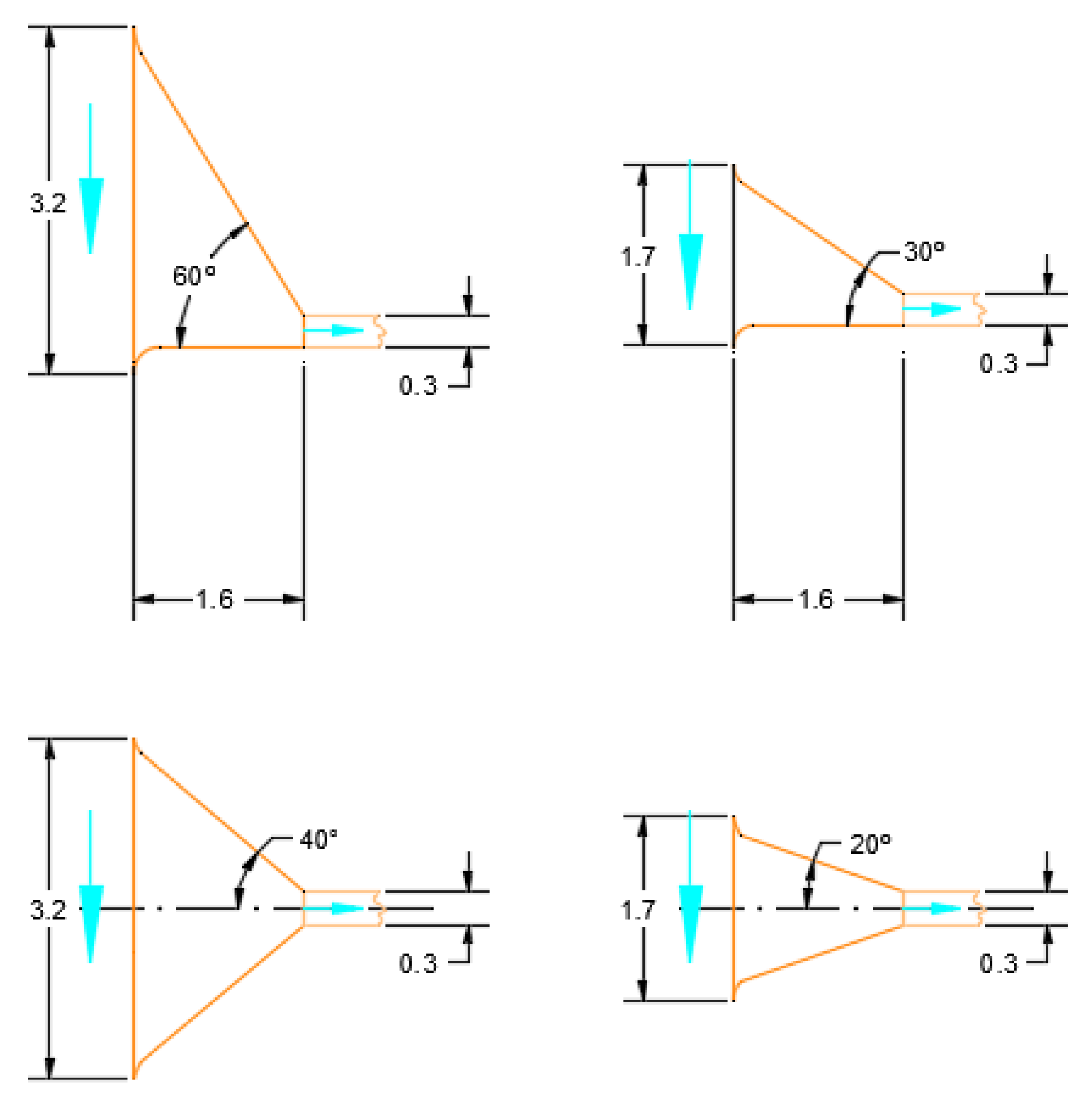
4.2. Nozzle Size
In this section, the effect of the size of the nozzle (
Figure 2) is studied.
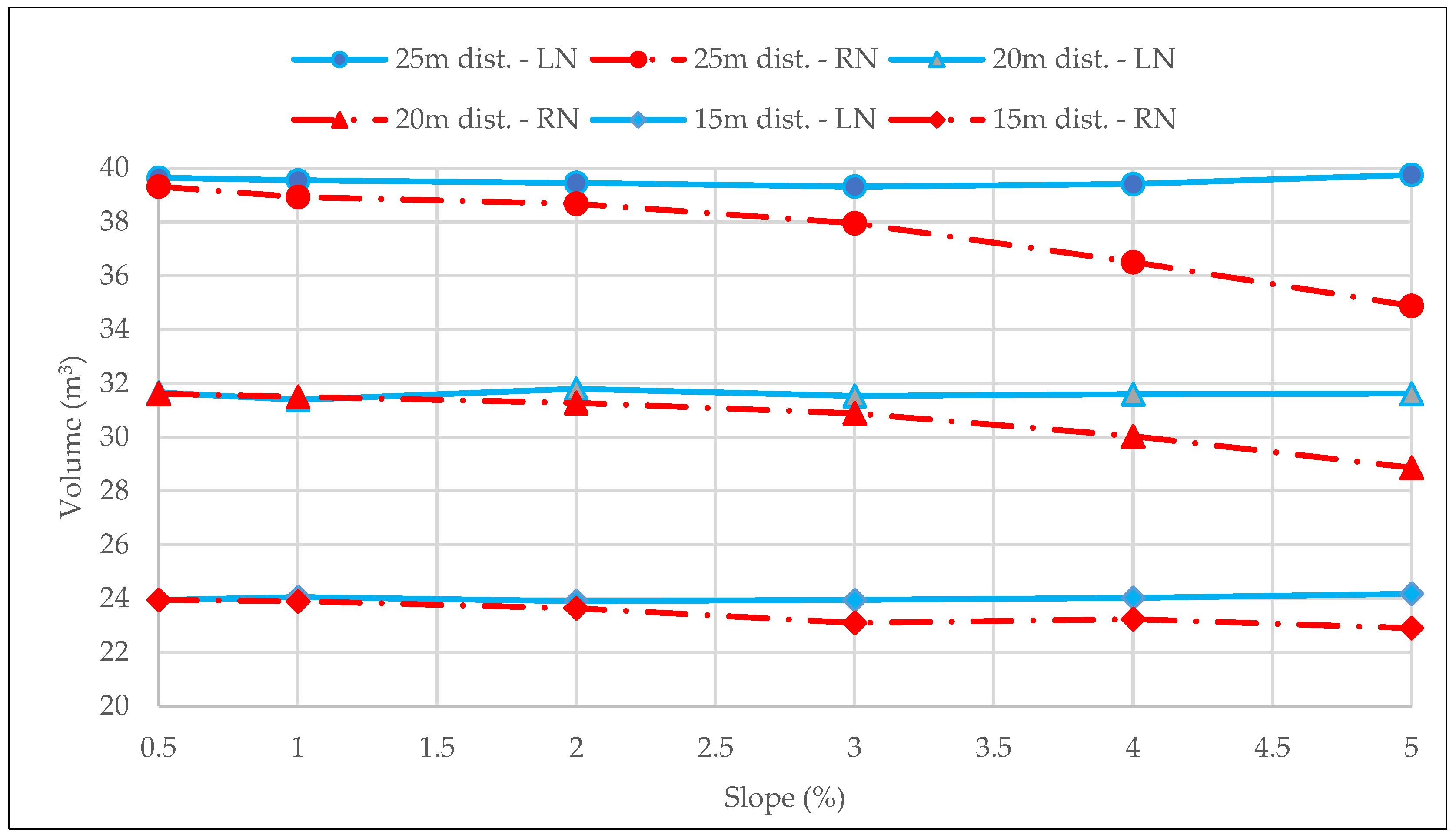
Figure 5 and
Figure 6 show the volume evacuated by each nozzle (considering equal drainage area) for both nozzle typologies and all longitudinally considered slopes.
As can be seen in
Figure 5 and
Figure 6, when the slope is equal to or less than 2%, both nozzles have equal hydraulic capacity. However, for slopes greater than 2%, the small nozzle presents a decrease in its hydraulic capacity that increases with the slope. This phenomenon can also be seen when comparing
Figure 5 and
Figure 6. For small nozzles, the volume evacuated by B1 is higher than B2 due to the lower hydraulic capacity of the reduced nozzle, which causes an increase in the gutter water level and, thus, in the flow evacuated by B1, since this is proportional to the water level.
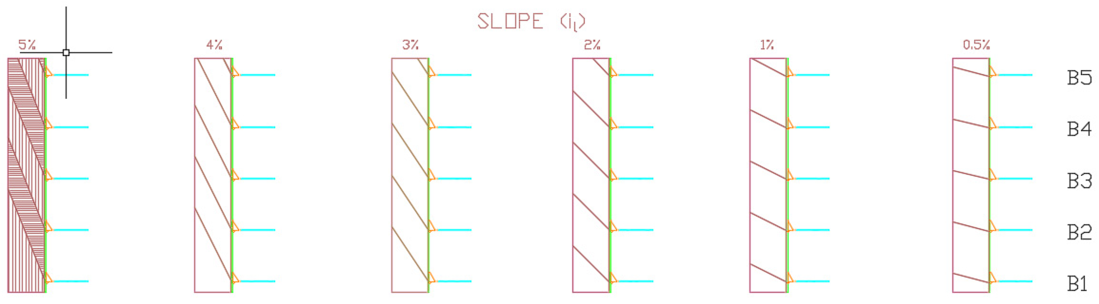
4.3. Longitudinal Slope
This section shows the influence of the longitudinal slope on the elements that constitute the drainage of the platform: the gutter, nozzle, and downspout.
Table 7 and
Table 8 show the maximum water depth reached in the model with a 30 cm wider gutter, combining different longitudinal slopes and embankment downspout distancing for a large and a reduced nozzle, respectively.
Table 9 and
Table 10 show the maximum water depth reached in the model with a 20 cm wider gutter, combining different longitudinal slopes and embankment downspout distancing for a large and a reduced nozzle, respectively.
In view of the results, it can be concluded that the 30 cm wide downspout satisfactorily meets any type of design; that is, it is not a conditioning element, reaching maximum values of 6.3 cm for a minimum slope of 0.5%, a 20 cm wide gutter, and a large nozzle.
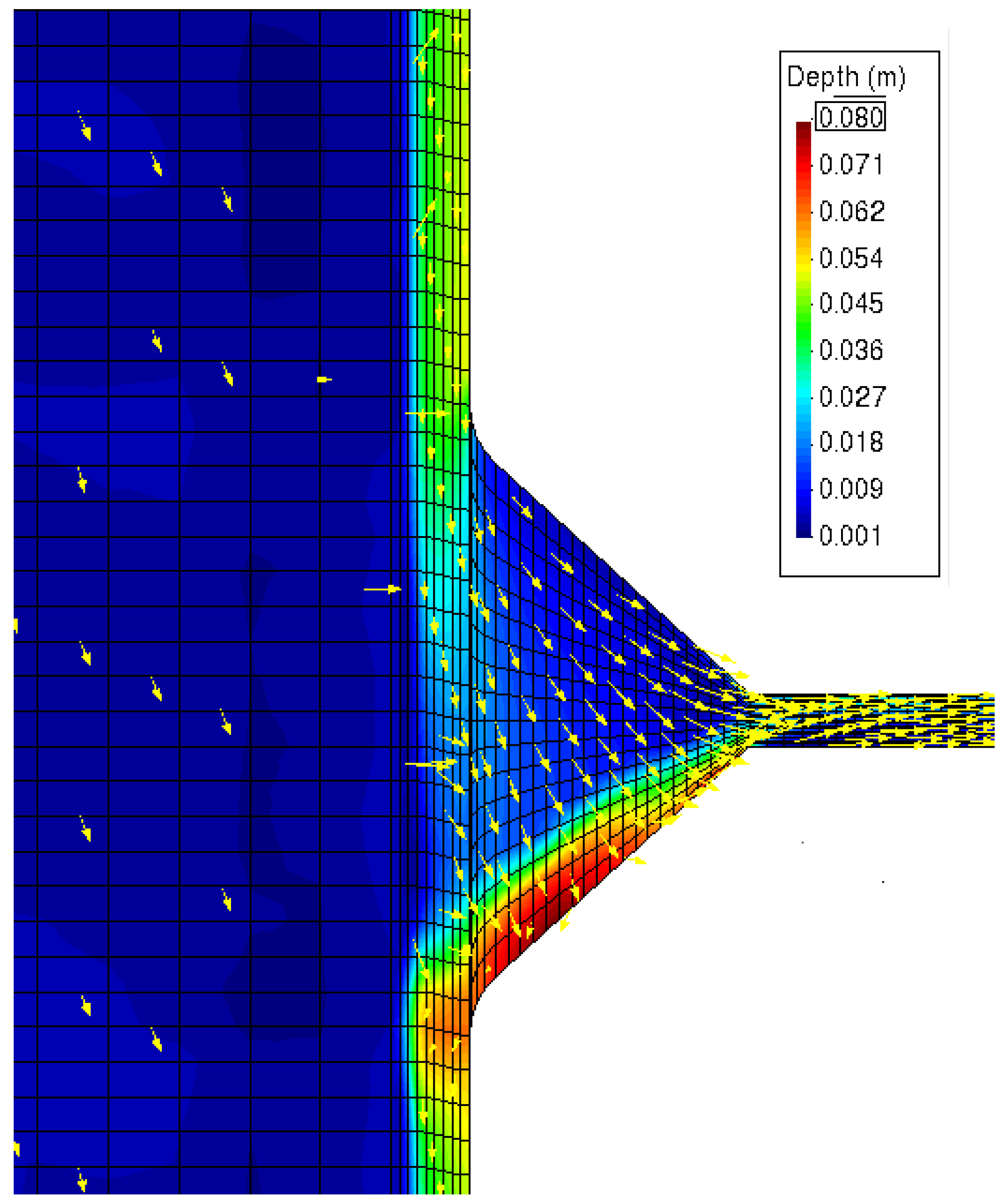
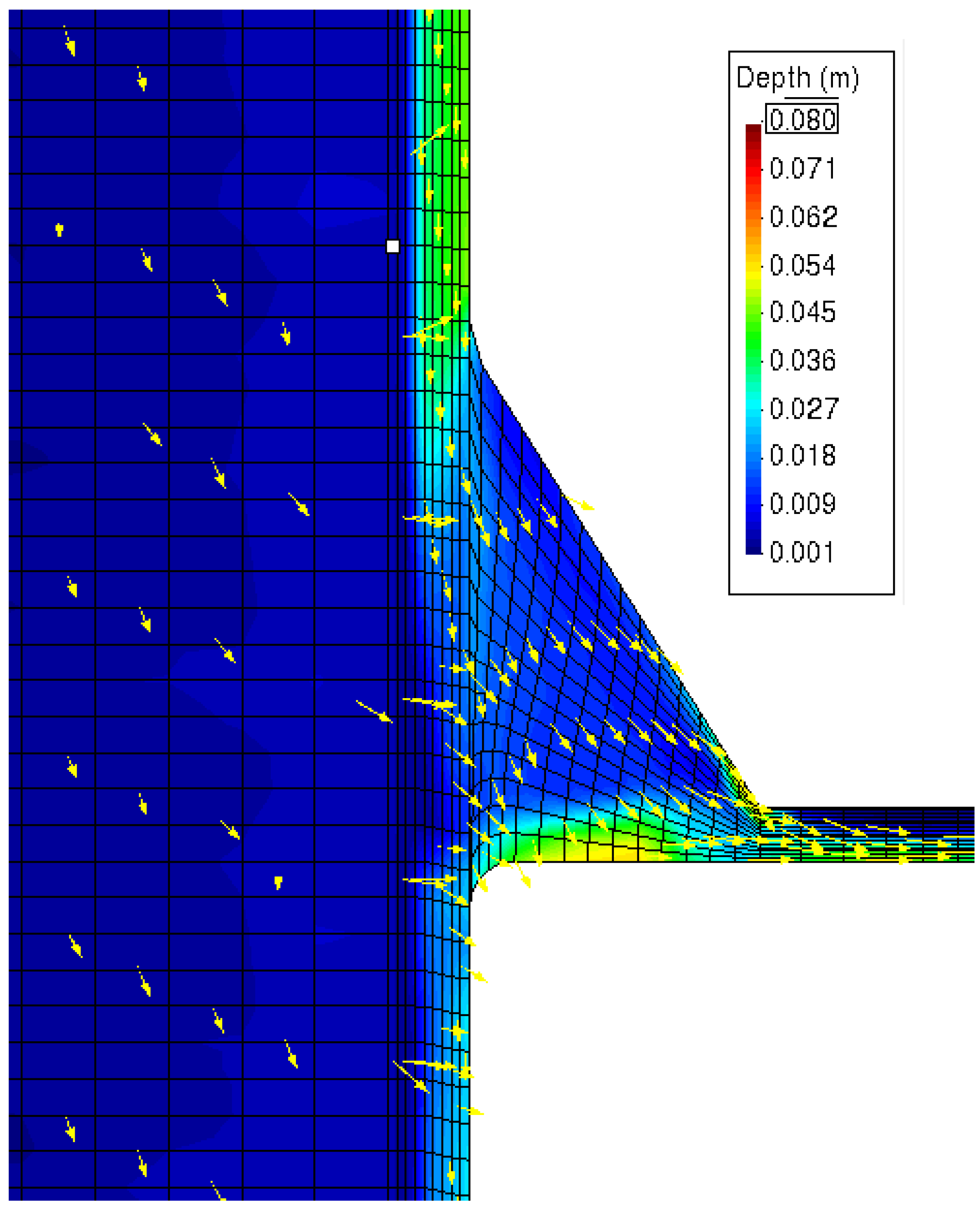
Finally, the slope considerably influences the nozzle water depths. For low slopes (<2%) and low velocities, the flow follows the edge of the nozzle inlet. However, for slopes greater than 3%, the flow is concentrated on the opposite edge of the inlet (
Figure 7).
4.4. Gutter Width and Embankment Downspout Distancing
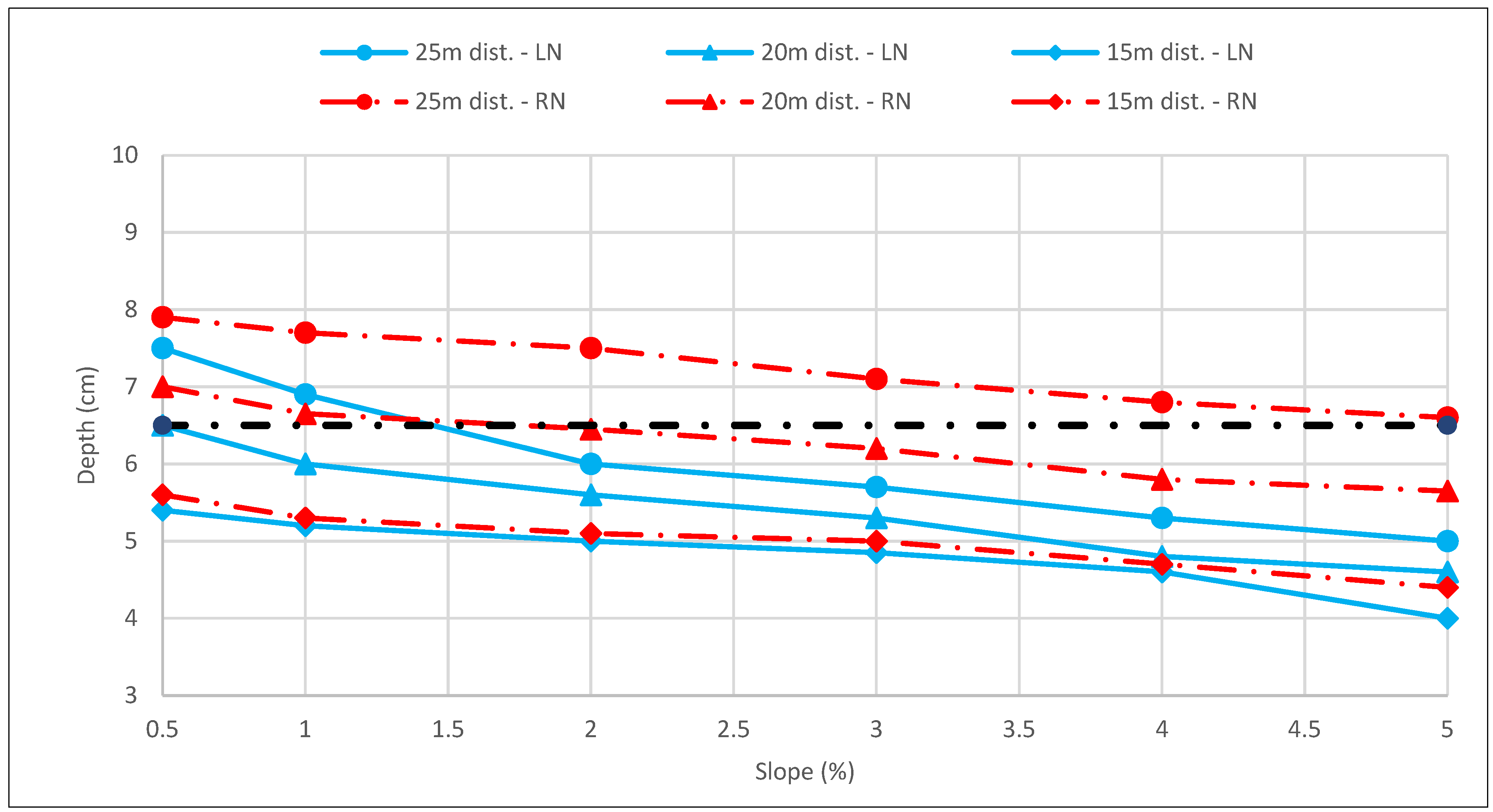
The influence of the gutter width and the embankment downspout distancing on the gutter are those associated with the flow velocity and depth in a channel. As the slope increases, there is a decrease in the water depth (
Figure 8) and, consequently, an increase in velocity.
This information is relevant since it conditions the suitability of the design because, according to Instruction 5.2-IC, this maximum water depth must have a guard on the shoulder platform greater than 5 cm.
Thus, for a 30 cm wide gutter, the guard is variable depending on the slope. As a summary, it can be concluded that, for slopes of less than 1%, downspout separations of 15 m can be used for both reduced and large nozzles, and if the separation is 20 m, only large nozzles should be used. For slopes greater than 2%, downspouts must be installed every 15 or 20 m with reduced or large nozzles.
Notwithstanding, for a 20 cm wide gutter, the scenario is different (
Figure 9). Separations of 15 m can be used with large nozzles for slopes of less than 1% and reduced nozzles for slopes between 1% and 5%. For separations of 20 m between downspouts, large nozzles can be used at 1.5% and reduced nozzles at slopes greater than 3.5%. Lastly, separations between downspouts of 25 m can only be used with large nozzles and with slopes greater than 2.5%.
4.5. Nozzle Type: Symmetrical and Asymmetrical
In this section, the influence of the nozzle type is analyzed: symmetrical vs. asymmetrical (
Figure 2) performance was compared in a model with 3 m downspouts with a 20 m separation between them.
The results indicate that for slopes ≤ 1%, the hydraulic capacity obtained in both cases is practically the same. However, for greater slopes, the hydraulic capacity of the symmetrical nozzle decreases progressively (
Table 11).
Figure 10 shows the comparison between the longitudinal profile in the gutter when symmetrical and asymmetrical nozzles are arranged for a longitudinal slope of 5%, where a considerable increase in the water depth is observed at the exit of the symmetrical nozzle compared to the asymmetrical one. The water depth in the gutter increases slightly on slopes ≥ 3%, and it presents a better distribution in the nozzle on the asymmetrical one for all slopes (
Figure 11 and
Figure 12).
For the application to a practical case, the authors recommend the creation of a synthetic model in accordance with the geometry and the hydrological characteristics of the site, such as a design hyetograph with a time resolution of five minutes (according to the concentration times of each downspout catchment). Regarding the former, it is necessary to highlight the importance of an adequate design of the width of the road, shoulders, gutter, and slope, which depends on the section. The variation in the slope is easily modifiable since once the model is available, it is only necessary to assign heights from an external file (e.g., raster or meshing point cloud).
With all the above, the proposed methodology is easily applicable to any type of road to be dimensioned. Furthermore, this methodology is also applicable for infrastructure already built in order to determine the degree of efficiency of the existing drainage system, thus anticipating future problems related to the road safety of the platform.
The methodology presented here addresses the problem of platform drainage through a rigorous mathematical model. The authors, experts in hydraulic calculation, have reviewed the current calculation methods, reaching the conclusion that the current methodologies are based on empirical formulas to obtain the water depth and flow in each of the designed downspouts. However, the methodology proposed here provides water depth, speed, and flow at any point of the model in a rigorous way.
5. Conclusions
This work explores the design of drainage downspout systems on road embankments through two-dimensional hydraulic modeling. A methodology that enables an efficient design of both the outlet and the spacing between downspouts was proposed, facilitating an optimal reduction in the runoff on the platform.
The application of this methodology revealed that the volume of runoff evacuated is greater with lower longitudinal slopes and with lower separations between downspouts. In all cases studied, a gutter width of 30 cm and a large nozzle ensure total runoff evacuation, even for separations of up to 30 m.
The influence of the longitudinal slope on the drainage elements has been studied, revealing that the 30 cm wide downspout satisfactorily meets the requirements in any design typology, while the depths of the nozzles vary depending on the slope. In such cases, the water depth reaches maximum values of 6.3 cm for a minimum longitudinal slope of 0.5%.
The influence of nozzle size shows that for slopes greater than 2%, smaller nozzles have lower hydraulic capacity than the larger ones. A 30 cm wide gutter with slopes lower than 1% and downspout separations of 15 m can be used for any size of nozzles, while a 20 m separation should be used only for large nozzles. Where slopes are greater than 2%, downspouts must be installed every 15–20 m. On the other hand, for a 20 cm wide gutter and a downspout separation of 15 m, large nozzles can be used for slopes lower than 1% and reduced nozzles for slopes between 1% and 5%. In the case of downspout separation of 20 m between, large nozzles can be used for slopes of 1.5% and reduced nozzles for slopes greater than 3.5%. Lastly, separations between downspouts of 25 m can only be used with large nozzles with slopes greater than 2.5%.


