Article

Simulation of Contaminant Transport through the Vadose Zone: A Continuum Mechanical Approach within the Framework of the Extended Theory of Porous Media (eTPM)

1
Institute of Structural Mechanics and Dynamics in Aerospace Engineering, Faculty of Aerospace Engineering and Geodesy, University of Stuttgart, Pfaffenwaldring 27, 70569 Stuttgart, Germany
2
Porous Media Laboratory, Institute of Structural Mechanics and Dynamics in Aerospace Engineering, Faculty of Aerospace Engineering and Geodesy, University of Stuttgart, Pfaffenwaldring 27, 70569 Stuttgart, Germany
*
Author to whom correspondence should be addressed.
Water 2023, 15(2), 343; https://doi.org/10.3390/w15020343
Submission received: 23 November 2022 / Revised: 5 January 2023 / Accepted: 10 January 2023 / Published: 13 January 2023
(This article belongs to the Section Water Quality and Contamination)

Abstract

:
The simulation of contaminant transport through the vadose zone enjoys high significance for decision makers and contaminated site planners since the vadose zone can serve as a filter, but many contaminants can be transported from this region to aquifers. The intention of this paper is to utilize the extended Theory of Porous Media (eTPM) to develop a ternary model for the simulation of contaminant transport in the vadose zone whose application is subsequently shown via a numerical example. The simulation was conducted for 140 days, during which the contamination source was removed after 25 days. The results indicate that the contaminant reached the water table after 76 days. The concentration of the contaminant reaching the groundwater was 17% less than that of the contaminant source.

1. Introduction

The vadose zone is the connection point between the surface of the earth, precipitation, surface water, and aquifers and enjoys great significance in the hydrological cycle, including water and energy in the land surface system of the earth [1,2]. This zone adjusts the water flow from the land surface to the groundwater and vice versa, and it plays a crucial role in the transport of solutes and their retention. The most severe contamination threats to groundwater quality emanate from coincidental surface releases of various types of wastes and products associated with industrial, agricultural, or urban development, such as leachate from municipal landfills [3]. These contaminants are transferred through the vadose zone, which is partially saturated with air and water. Although the vadose zone functions as a buffer and filter zone, in which attenuation, absorption, screening, degradation as well as chemical and biological transformations of contaminants occur, most of the hazardous contaminants are reactive in soil, and they infiltrate through the vadose zone and permeate unsaturated soil in order to reach the aquifer and continue to migrate in the direction of the groundwater flow [4]. Hence, the contamination of the vadose zone can be considered as a continuous source of contamination for aquifers, and it affects the quality and quantity of groundwater resources [5,6], leading to significant risks for human health and the environment.
The risk assessment, which is required by decision makers for the long-term management of the contaminated vadose zone, necessitates an understanding of the water flow and the fate of contaminants and their concentration at certain points [7]. Because the direct measurement and monitoring of contaminants’ concentration and the impact of a contaminated vadose zone on the groundwater quality are difficult and costly processes in many cases, mathematical modelling methods can instead be employed to quantify such impacts. Furthermore, the results of such models can be utilised for testing alternative conceptual models, predicting future conditions, providing information required for remediation design, interpreting and analysing field experimental data, and subsequently evaluating corrective measures.
In view of this, several mathematical models have been developed based on various analytical and numerical studies. In general, there are two different approaches to the simulation of flow and contaminant transport in the vadose zone, namely analytical [8,9,10] and numerical methods [11,12]. Due to the complexity of phase partitioning and reaction, there are only a few analytical models considering multiple phases and multiple solutes [13,14], multiple solute transport with reactions in multiple phases [15], and combined transient water and solute transport [16]. In order to deal with problems concerning saturated and unsaturated zones, there are different numerical approaches, including the finite difference method (FDM) [17,18], the finite volume method (FVM) [19], the finite element method (FEM) [20,21], and the Meshfree method [22], each of which has various treats that tailor the model to the special application for which it was designed. Rao et al. combined explicit finite difference formulations with multiple domain algorithms and developed models for one and two-dimensional transient contaminant transport flow [23,24]. Kačur et al. introduced a continuum mechanical model for fluid flow in unsaturated deformable porous media, where the fluid could undergo phase transitions [12]. Kuntz et al. developed a numerical simulation of the reactive transport of compounds in the vadose zone to investigate whether steady-state flow simulations accurately describe reactive contaminant transport under transient conditions in the field [25]. Bunsri et al. developed a model for water movement and contaminant transport through unsaturated soil based on Richard’s equation and utilizing the finite element method [26]. Rajsekhar et al. described virus transport in partially saturated soil using the finite volume method; they considered the virus sorption on the liquid–solid and air–liquid interfaces as well as the inactivation of viruses suspended in the liquid phase and viruses attached to both interfaces [27]. Furthermore, different software packages, including HYDRUS, Modeflow, and Chemflux, have been developed over the last few years, each having its own advantages and disadvantages [28,29]. HYDRUS describes the vadose zone process using the one-dimensional Richards equation, which requires moderate computational effort [30].
Most of the flow and contaminant transport models of the vadose zone do not consider the entire coupling of the thermo–hydro–mechanical interaction, phase transitions, deformability of the soil, physical phenomena concurrent with water flow, air flow, heat transfer, and contaminant transport, and in particular, the effects of air flow, temperature, and chemical reactions. The Theory of Porous Media (TPM) [31,32,33,34] facilitates a comprehensive continuum mechanical framework based on the Mixture Theory [35], enhanced by the concept of volume fractions, for the simulation of different processes in a saturated or partially saturated medium. Furthermore, it paves the way for the description of geophysical and geochemical environmental problems [18,21,36,37,38,39,40,41,42].
This study aims to provide a numerical simulation of contaminant transport in the vadose zone within the framework of the extended Theory of Porous Media. In developing the simulation, the vadose zone is modeled as triphasic system consisting of a soil phase ( S ) , saturated by water as a liquid phase ( L ) and a gaseous air phase ( G ) . The phases are assumed to be immiscible and statistically and homogeneously distributed over the control volume. Each phase can be composed of or can contain miscible components, which can be considered as contaminants. Their motion through porous media in regard to different transport regimes, such as diffusion and advection, can be simulated.
In this paper, the development of a triphasic model based on the Theory of Porous Media (TPM) is initially presented. The model is expanded by considering a contaminant as a solute in the water utilizing the extended Theory of Porous Media (eTPM). For the conceptual and numerical testing of the model, a numerical example is considered and its simulation results are presented.

2. Materials and Methods

2.1. Theory of Porous Media (TPM)

The fundamentals of the TPM were developed from the combination of two basic concepts, namely the Theory of Mixtures [43] and the concept of volume fractions [44,45,46], which enable the consideration of the local composition of the overall aggregate. The vadose zone as a partially saturated soil, denoted as φ , is composed of phases φ α with α { S , L , G } , namely pure soil as a solid ( S ) matrix, which generates the control volume B S and its boundary B S , saturated by a fluid ( F ) which consists of liquid ( L ) and gas ( G ) , expressed as follows:
φ = α φ α = φ S φ F , where φ F = φ L φ G .
The TPM utilizing the Theory of Mixtures smears each heterogeneously distributed constituent of the true structure over a control volume. The applied homogenization procedure of each phase of the vadose zone over a representative elementary volume (REV) leads to the ternary superimposed continuum model, see Figure 1.
As a consequence of the superposition of the homogenized phases, each phase φ α occupies each spatial point of the control volume simultaneously. The volume fraction n α of each phase is defined with
n α x , t = dv α dv ,
where x denotes the position vector in the current configuration at time t , dv α is the partial element volume of the phase φ α , and dv is the element volume of the bulk medium [32,38]. With the definition of the volume fraction, which assigns a volumetric dimension to each phase in every spatial point x , each phase can be identified within the mixture. Due to the applied homogenization, the partial density ρ α is defined as the partial mass dm α of phase φ α divided by the bulk volume dv , expressed by
ρ α = dm α dv .
With Equation (2), the partial and realistic density ρ α R are connected via
ρ α = n α ρ α R .
Regarding the constraint that no vacant space within the control volume B S is allowed, and with the result that the solid matrix is entirely saturated by the fluid phases water and air, the saturation condition can be written as
α = 1 κ n α x , t = α = 1 κ dv α dv = α = 1 κ ρ α ρ α R = 1 ,
where x denotes the position vector in the actual configuration of the material point X α .
Balance equations describe the equilibrium condition that each natural system strives for. Applied mechanics deals with four balance equations, which draw a conclusion from the mass, the momentum, the moment of momentum, and the energy of a continuous body. Analogously to a single-component material, these balance equations can be written for all phases in the framework of the TPM, considering all interactions for the description of chemical and physical exchange processes, such as the mass or energy exchange between the phases. The balance equations in the aforementioned order can be written as follows:
n α α ρ α R + n α ρ α R α + n α ρ α R div x α = ρ ^ α ,
div T α + ρ α ( b x α ) = ρ ^ α x α p ^ α ,
T α = T α T ,
ρ α ε α α T α · D α ρ α r α + div q α = e ^ α p ^ α · x α ρ ^ α ( ε α 1 2 x α · x α ) .
The quantities ρ ^ α , p ^ α , e ^ α , ε α , r α , q α represent mass, momentum, and energy supply, as well as the specific internal energy, an internal heat source, and the heat flux over the surface, respectively. Moreover, b , D α and T α denote the body force vector, the symmetric part of the spatial velocity gradient, and the partial Cauchy stress tensor, respectively. The detailed kinematic relations are described in Appendix A. Since the sum of the local balance equations over all phases must comply with balance equations for a one-component material and for the whole mixture, the sum of the supply terms has to be zero [47]:
α = 1 κ ρ ^ α = 0 , α = 1 κ p ^ α = o , α = 1 κ e ^ α = 0 .
The specific internal energy ε α can be rewritten in terms of the Helmholtz free energy function ψ α and the specific entropy η α with the following equation:
ε α = ψ α + θ α η α ,
where θ α is the absolute phase temperature. Establishing the common entropy inequality for all phases is a necessary and sufficient condition for the existence of a dissipation mechanism within the mixture [32] and provides thermodynamically consistent restrictions for constitutive modelling. Hence, the entropy inequality must be evaluated for the whole mixture by the sum over all κ phases with the following equation:
α = 1 κ ρ α η α α + ρ ^ α η α α = 1 κ [ 1 θ α ρ α r α div ( 1 θ α q α ) ] ,
where ’div’ denotes the spatial divergence operator.

2.2. Extended Theory of Porous Media (eTPM)

To represent miscible substances within the macroscopic immiscible phases φ α , the TPM has to be extended [48]. The extended TPM (eTPM) offers a comprehensive approach for the simulation of different physical and chemical processes, such as the transport processes of miscible substances, i.e., solutes, in their carrier phases (solvents). On the basis of the eTPM, the composition of the porous medium, which is the object of our investigation, can be rewritten as
φ = α φ α with φ α = β φ α β .
where φ α β denotes the ν miscible substances φ β solved in the carrier phase φ α . To consider the contribution of the solute to the whole mixture, the mixture molar concentration and the solvent molar concentration of the solute can be defined as follows:
c mol β = dn mol β dv ,
c mol α β = dn mol β dv α ,
where dn mol β = dm β \ M mol β denotes the number of moles, while dm β and M mol β define the local mass of a solute φ β in terms of the molar mass. Analogously to Equations (3) and (4), different mass densities can be defined for the miscible components. The mass concentration of component ρ β in the solvent ρ α is given with
ρ α β = dm β dv α ,
and its partial density as
ρ β = dm β dv = dv α dv dm β dv α = n α ρ α β .
The mass and molar concentration (Equations (15) and (16)) are connected via the molar mass with
ρ α β = c mol α β M mol β .
In analogy to the macroscopic and immiscible quantities, the balance equations, kinematics, and constraints of the supply terms are valid for the mixture components.

2.3. Model Assumptions

The vadose zone is composed of the soil matrix φ S saturated by water, represented by the liquid phase φ L , and by air, represented by the gas phase φ G . The liquid phase is composed of the contaminant φ LC solved in the carrier phase φ L , so that the mixture body under investigation can be described with
φ = φ S φ L φ LC φ G
Since the volume fraction of the water contaminant is negligible in comparison to that of the carrier phases, no volume change dependent on a concentration variation is considered, and the saturation condition is given as follows:
n S + n L + n G = 1 .
For the description of the biphasic fluid mixture, it is convenient to introduce the saturation function s β , which defines the ratio of the pore fluids in the available pore space with
s β = n β n F , β { L , G } ,
where n F = n L + n G denotes the porosity variable, which leads to
s L + s G = 1 .
Therein, s L and s G denote the saturation degrees of the liquid and gas phases, respectively.
Soil and water are considered to be incompressible; thus, their realistic densities ρ S R and ρ L R are constant, resulting in ρ S R S = ρ L R L = 0. The air is assumed to behave as an ideal gas, and its density change depends on the temperature θ and the effective air pressure p LR , with ρ L R = ρ L R θ , p L R . Mass transfer is not taken into consideration, such that
ρ ^ S = ρ ^ L = ρ ^ G = 0 .
The constraint for the interaction forces (Equation (10) 2 ) evaluated for the investigation of the contaminated vadose zone reads
α = 1 κ p ^ α = p ^ S + p ^ F = o ,
with
p ^ F = p ^ L + p ^ LC + p ^ G .
All constituents investigated contain the same temperature with θ S = θ L = θ L . Thus, there is no energy supply e ^ α between the phases, such that Equation (18) 3 vanishes with
e ^ S = e ^ L = e ^ G = 0 .
Additionally, both a constant temperature and no internal heat supply source r α are considered, so that the energy balance within the set of governing equations can be excluded. Moreover, quasi-static conditions are assumed for all macroscopic phases as well as for the contaminant, so that the acceleration terms can be neglected. Although this restricts the validity of the model to slow processes, it represents a reasonable assumption since acceleration terms fundamentally enact no part for the vadose zone, except in some circumstances such as during an earthquake. In addition, the square of the velocities x α · x α and x LC · x LC are not taken into consideration.

2.4. Field Equations

Considering the introduced assumptions, the quasi-static, triphasic, multi-component model is derived to describe water flow and contaminant transport in the vadose zone. A set of coupled field equations, balance equations of mass and momentum, is required to calculate the unknown quantities while considering the restrictions associated with the volume fractions and interaction forces. The local forms of the mass balance equations for the solid, liquid, and gas phase are given with
n F S + n F 1 div x S = 0 , n F s L S + n F s L div x S + div n F s L w L S = 0 , n F s L ρ L R S + n F s L ρ L R div x S + div n F s L w GS = 0 ,
where w L S = x L x S and w G S = x G x S denote the relative difference velocities between the liquid and gas phase, and the solid deformation. The local mass balance equation of the contaminant is derived as
n L c mol LC M mol C LC + n L c mol LC M mol C div x LC = 0 .
Considering the constant molar mass M mol C and the time derivative with respect to the solid phase leads to
n F s L S c mol LC + n F s L c mol LC S + div j mol LC + n F s L c mol LC div x S = 0 ,
where j LC mol = n F s L c mol LC w LC S indicates the molar flux of the contaminant, which is given with the difference velocity w LC S = x LC x S . Considering the given assumptions, the partial local momentum balance equations for the individual phases and the contaminant read as follows:
div T S + 1 n F ρ S R b = p ^ S , div T L + n F s L ρ L R b = p ^ L , div T G + n F s G ρ G R b = p ^ G , div T LC + ρ LC b = p ^ LC .

2.5. Constitutive Model

In addition to the kinematics and balance equations, constitutive equations are required in order to complete the system of equations and to identify and define the partial Cauchy stress tensors T S , T L , T G and T LC , the linear momentum productions p ^ G , p ^ L , and p ^ LC , the saturation s L and the effective gas density ρ G R . Proceeding from general thermodynamical considerations [49,50] and the evaluation of the entropy inequality (see Appendix B), the partial Cauchy stresses are given with the following relations:
T S = 1 J S λ S ln J S I + μ S K S n S p F R I , T L = n L p L R I + T LC , T LC = n L μ LC I , T G = n L p G R I .
In the equation above, K S = 1 2 B S I denotes the Karni–Reiner strain tensor, with B S = F S F S T being the left Cauchy–Green tensor. The quantities p LR , p GR , and p F R denote the effective pressure of the wetting pore water, the effective pressure of the non-wetting pore air, and the effective overall fluid pressure, respectively, and μ L C denotes the chemical potential of the contaminant.
Incorporating the momentum production terms into the corresponding momentum balances, the individual relation for the filter velocities, which can be defined as the product of the volume fraction (see Appendix A.2), are given as follows:
n G w GS = k r G μ G K S [ grad p G R + ρ G R b ] ,
n L w LS = k r L μ L K S [ grad p L R + ρ L R b ] ,
where μ G and μ L indicate the shear viscosity of air and water, K S is intrinsic soil permeability, and k r G and k r L are the relative permeability of air and water. These relations represent the standard Darcy law derived from the experiments for the multi-phase flow problems [51]. In addition, the flux of the contaminant in the water can be established with
j mol LC = n L c mol LC w LC S = D Fick 1 R θ grad μ LC + n L c mol LC w L S
where D Fick , R and θ denote the diffusivity of the contaminant within the water, universal gas constant and absolute temperature.

2.6. Numerical Treatment

By utilizing the FEM in the framework of a standard Galerkin procedure, the weak formulation of the local balance equations is formulated. The transformation of the strong local form of the mechanical balance equations into a weak global representation is realised by multiplying them with the following independent weighting functions:
W = { δ u S , δ p L R , δ p G R , μ LC } .
In order to derive the weak formulation of the momentum balance of the overall mixture, this equation is multiplied scalar by the respective test function δ u S representing a virtual deformation of the solid phase. Integrating over the domain B S and restating the term governed by the divergence operator by utilizing the product rule and the Gaußian integral theorem yields the weak formulation as
B S α S , L , G T α · grad δ u S d v B S α S , L , G ρ α b · δ u S d v = B S t · δ u S d a .
Therein, T LC is neglected (cf. Appendix A.1). The surface integral appears, which is governed by the overall surface traction t = T S + T L + T G n acting on the so-called Neumann boundary B S of the overall mixture.
Analogously to the overall momentum balance, the weak forms of the volume balances of the water and air can be derived by weighting them with the test functions δ p LR and δ p G R , respectively. This yields
B S n L w LS · grad δ p L R d v B S n L S + n L tr D S δ p L R d v = B S n L w LS · n δ p L R d a .
and
B S n G ρ G R w GS · grad δ p G R d v B S n G ρ G R S + ρ G R n G S + n G ρ G R tr D S δ p G R d v = B S n G ρ G R w GS · n δ p G R d a ,
where n L w LS · n and n G ρ G R w GS · n denote the flux of the water volume and air mass through the Neumann boundary B S . The weak form of the concentration balance for the solute is derived with
B S n L c mol L C S δ μ L C d v B S j mol L C · grad δ μ L C d v + B S n L c mol L C tr D S δ μ L C d v = B S j mol L C · n δ μ L C d a .

3. Results and Discussion
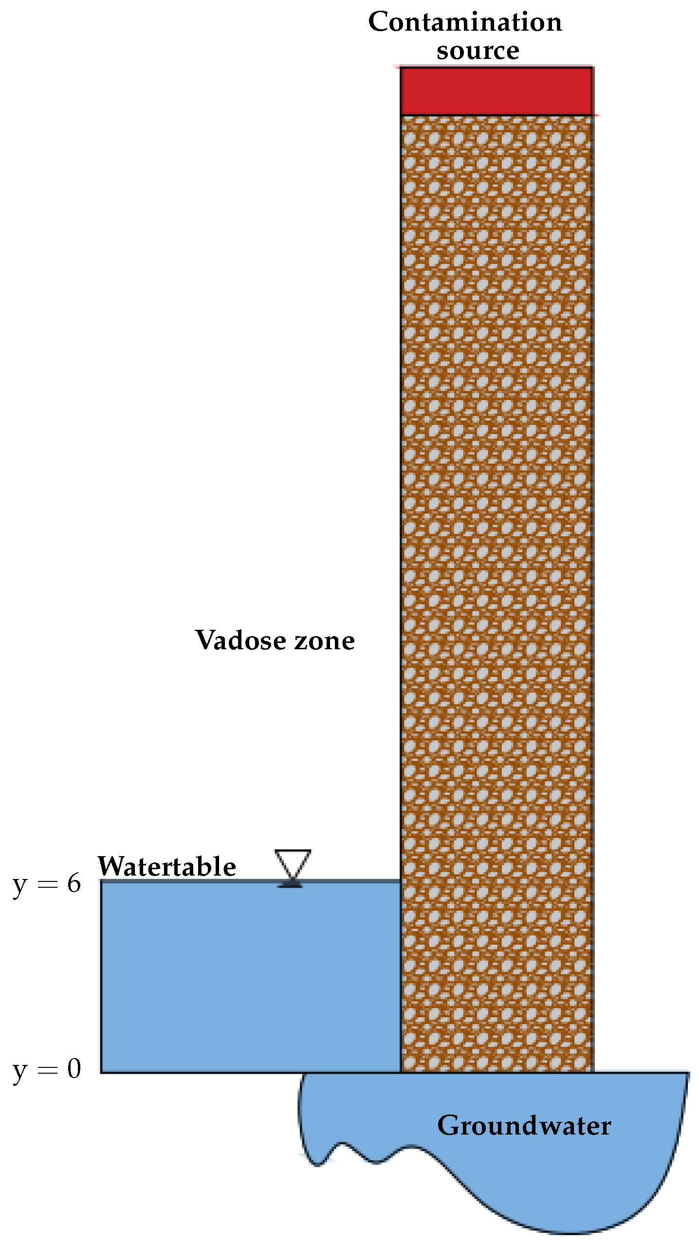
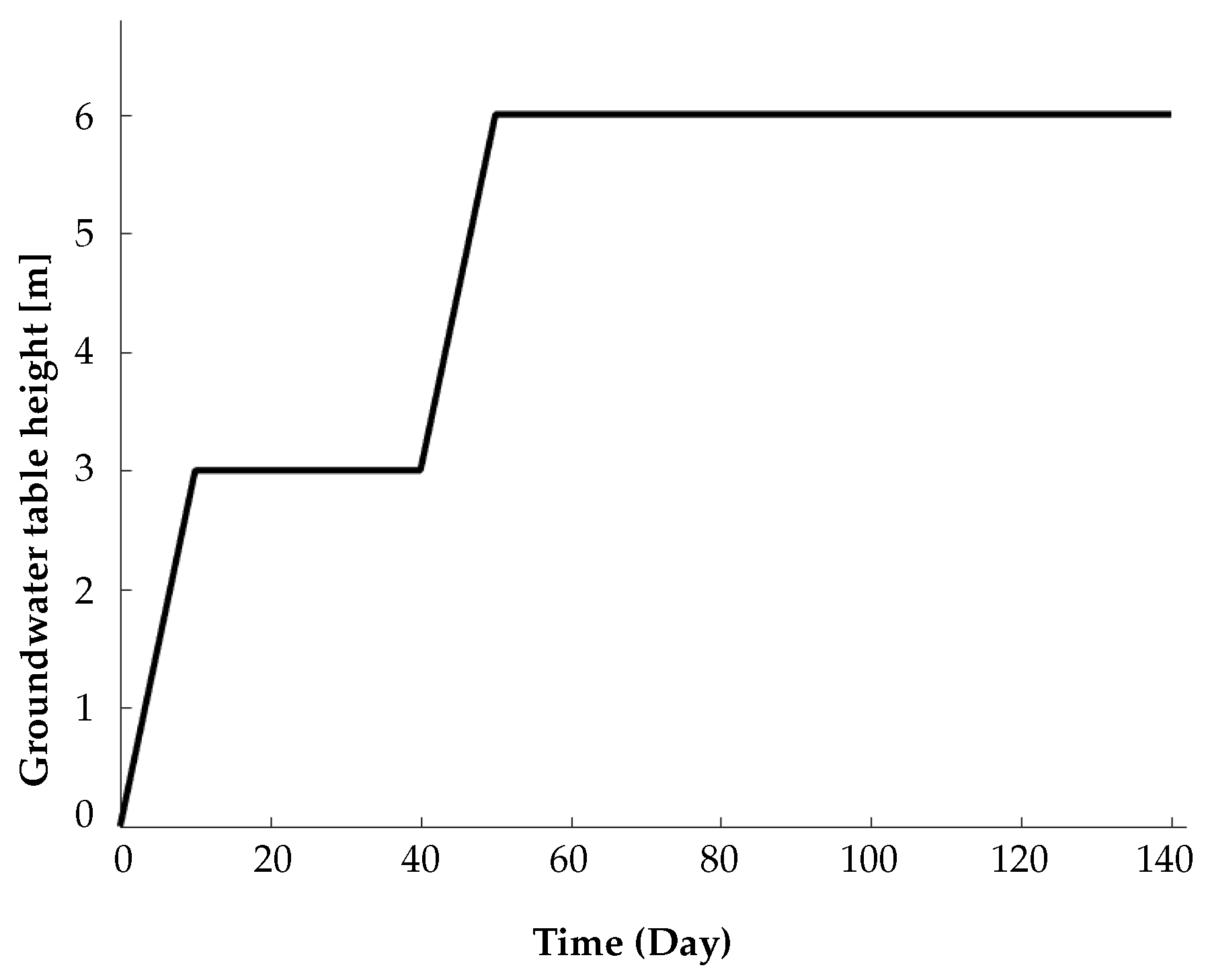
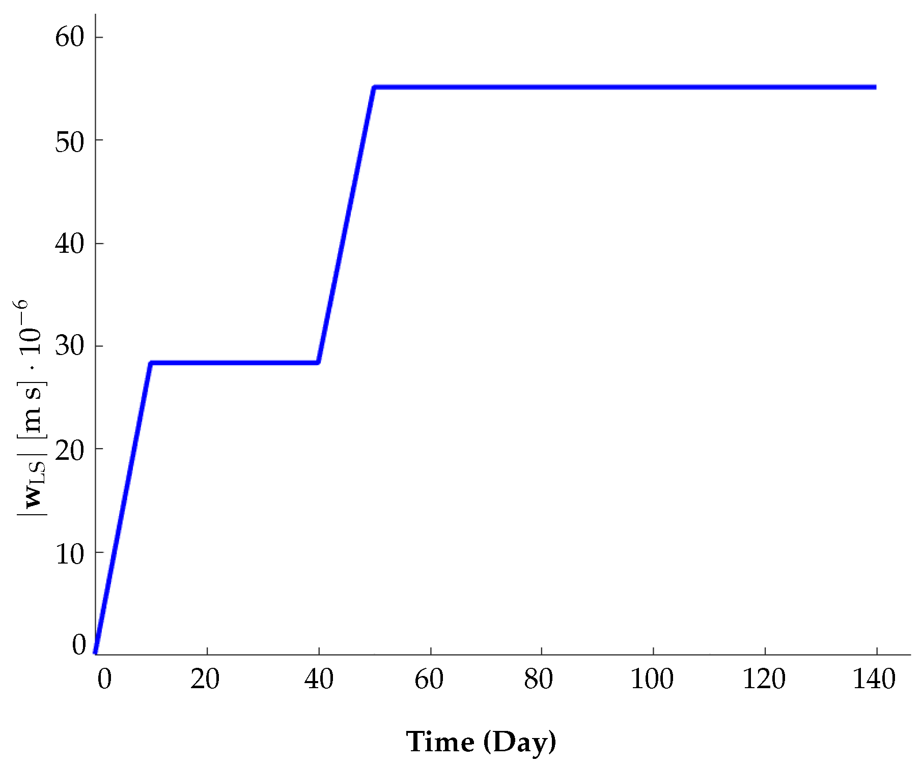
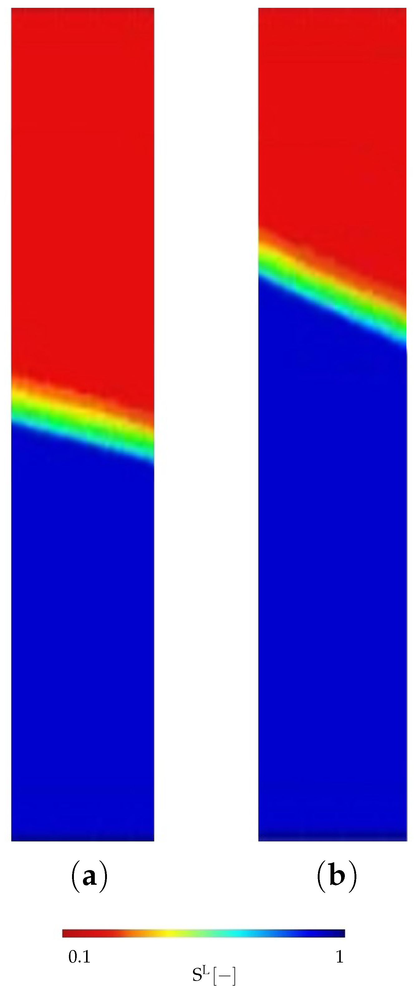
The simulation of contaminant fate in the vadose zone is an ongoing research topic, wherein a variety of numerical studies are performed to determine the dynamics of the vadose zone. The computations presented here resulted from a triphasic TPM formulation; they were used together with the numerical tools presented in the previous sections and implemented into the finite element program FEAP, developed by Taylor, UC Berkeley. To ensure stable numerical results, the so-called Taylor–Hood elements were used with quadratic ansatz functions for the displacements, while the linear ansatz functions were used for the remaining degrees of freedom. The triphasic model was applied to a numerical example. Table 1 illustrates the material parameters and initial values, which were used to describe the vadose zone and contaminant transport.
The numerical example corresponds to a two-dimensional description of the contaminant transport through the vadose zone (cf. Figure 2). The vadose zone has a height of 40 m and a width of 5 m. Furthermore, the left side of the vadose zone is assumed to be more or less impermeable. In addition, the right side of the vadose zone is impermeable; only the last 10 m on the right side are permeable, and the filter on the right-hand side of the structure is assumed to be governed by K S = 10 8 m . The vadose zone is governed by an intrinsic permeability of K S = 10 10 m . Based on the triphasic formulation, it is assumed that a water table on the left side of the vadose zone is slowly increased. As a result, water streams into the vadose zone and finally reaches a stationary state.

Numerical Example

The level of the groundwater table can vary because of natural phenomena such as precipitation and oceanic oscillations such as tides and waves in the coastal aquifers [52]; the variation can also be caused by human activities. The change in the groundwater table is determinative of the variation of the saturation degree, seepage velocity, and contaminant fate. In order to develop a remediation process, it can be beneficial to know how varying the groundwater table and saturation degree in the vadose zone can affect the contaminant fate. Concerning this, the sketched vadose zone (see Figure 2) is numerically investigated together with the changing of the groundwater table on its left side. The example shows a two-dimensional description of the contaminant transport through the vadose zone to the water table. The investigated vadose zone has a dimension of 5.0 m × 40.0 m. The simulation was conducted for 140 days. The groundwater table on the left side of the vadose zone is slowly increased to the height of h 1 = 3 m within the time t 1 = 10 days ; thereafter, it is kept constant for a duration of 30 days . Afterwards, the groundwater table is further increased in height for another t 2 = 10 days , and then it is kept constant (see Figure 3). This leads to water flow in the x-direction. Figure 4 shows the change in | w L S | in the right corner of the vadose zone, which suits the change in the groundwater table on the left-hand side of the vadose zone. | w L S | increases each time with the rise of the groundwater table. When the groundwater table is constant, | w L S | remains constant, too. Figure 5 illustrates the distribution of the saturation degree s L and the pore fluid flow at different times prior to the stationary state. The water table gradually starts to increase with the increase of the groundwater table on the left side of the vadose zone. In the stationary state, the pore liquid saturation reaches its final distribution. The mesh has to be strongly refined in the zones with high gradients of effective saturation. The contaminant source was only available in the initial 25 days; it was subsequently removed. Figure 6 demonstrates the contaminant distribution within 140 days. During the first 40 days, the contaminant only moves downwards in the y-direction, without a gradient in the x-direction. The rising water table has no significant influence on the contaminant transport. Afterwards, the contaminant reaches the lower part of the studied vadose zone and begins to move in two directions, namely x and y. The maximum flux of the contaminant in the x-direction occurs in the lowest 8 m of the vadose zone, which is saturated after 78 days. The results indicate that the contaminant reached the groundwater after 76 days, in which 83% of the initial concentration entered the vadose zone. In the homogeneous horizontal contaminant transport situation, the plume must conform to an idealized wedge-like shape; however, in the vadose zone with the assumed boundary condition in this numerical example, the plume is completely deformed. When the contaminant flows over the vadose zone, there is no corresponding distortion for the wedge in the overall geometry of the system.

4. Conclusions

A comprehensive triphasic TPM model was developed to predict contaminant transport through the vadose zone. The developed model was applied to a numerical example, in which the contaminant source was removed after 25 days. The water level on the left boundary of the model rose from 0 to 6 m in 30 days. The results show that the contaminant has no flux in the x-direction at the highest level of 12 m. The contaminant flux increases as the contaminant moves downwards in the remaining 28 m. The concentration of the contaminant reaching the groundwater was 17% less than that of the contaminant source. The contaminant reached the ground water after 84 days. The study shows that the contamination of the vadose zone can be seen as a contaminant source for groundwater. The next step of this study could be the simulation of the filtration effect of the vadose zone and the reactive transport of contaminants through the vadose zone. The distribution of the pore gas suction is only possible if the formulation is triphasic. Moreover, the maximum gas suction can substantially affect the liquid flow situation. Despite the fact that it diminishes with time due to the gas inflow through the specimen’s top surface, this effect demonstrates the most significant distinction between the triphasic and biphasic formulations. The water efflux can also demonstrate the distinction between triphasic and biphasic formulations.

Author Contributions

Study concept and design: S.M.S. and T.R. Simulation and implementation of the model in FEAP: S.M.S. and A.T. Analysis of data: S.M.S. Interpretation of data: S.M.S. Writing manuscript: S.M.S. Critical revision: All authors. All authors have read and agreed to the published version of the manuscript.

Funding

This work was completed as part of the REMEDIATE (Improved decision-making in contaminated land site investigation and risk assessment) Marie-Curie Innovation Training Network. The network received funding from the European Union’s Horizon 2020 Programme for Research, Technological Development, and Demonstration, under grant agreement no. 643087. REMEDIATE is coordinated by the QUESTOR Centre at Queen’s University Belfast, http://questor.qub.ac.uk/REMEDIATE/. This work was funded by the Deutsche Forschungsgemeinschaft (DFG, German Research Foundation)—312860381 (Priority Programme SPP 1886, Subproject 12), 390740016 (Germany’s Excellence Strategy EXC 2075/1, Project PN 2-2A), and 436883643 (Research Unit Programme FOR 5151, Project P7).

Conflicts of Interest

The authors declare no conflict of interest.

Abbreviations

The following abbreviations are used in this manuscript:
eTPMExtended Theory of Porous Media
REVRepresentative Elementary Volume
TPMTheory of Porous Media

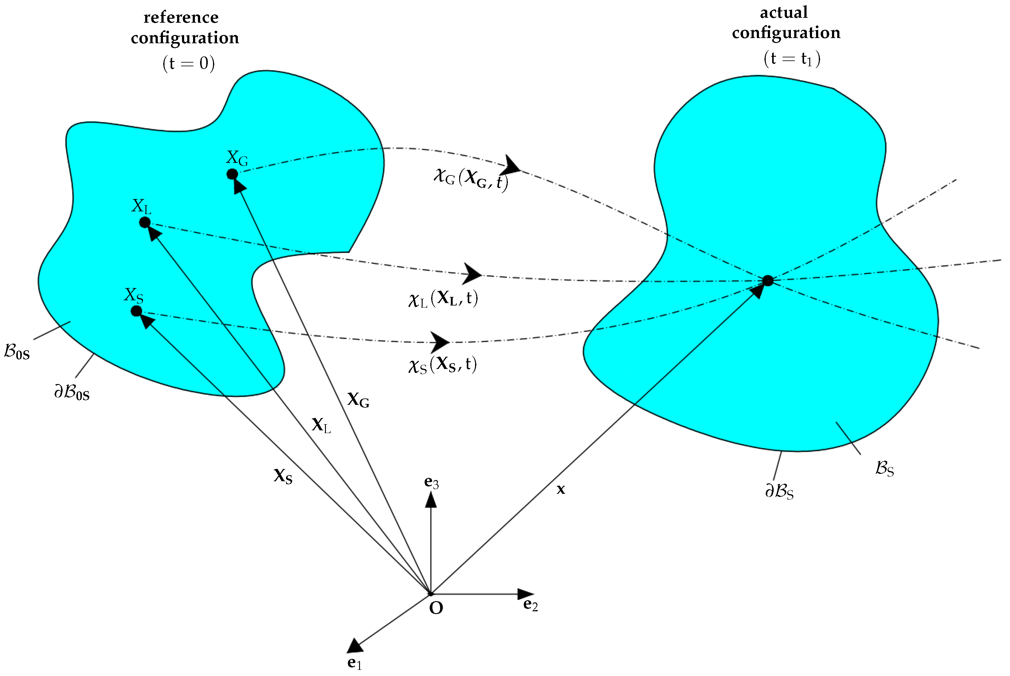
Appendix A. Kinematic

In considering of the vadose zone as a multi-phase material, the smearing of the constituents over the whole domain implies that in the actual configuration, each spatial position x of the domain is simultaneously occupied by all constituents–all material points X S , X L , and X G . The requirement of having independent states of motion for the constituents implies that each particle does not necessarily trace back to a common reference position, but it can have individual reference positions X α (see Figure A1). Thus, each constituent is allocated to its own independent motion function χ α as follows:
X α = χ α 1 ( x , t ) if det ( χ α X α ) 0 .
The velocity and acceleration fields for each constituent are introduced by using the material time derivatives in a Lagrangean setting expressed with
x α = χ α ( X α , t ) t , x α = 2 χ α ( X α , t ) t 2 .
The material deformation gradient F α and its inverse can be obtained as follows:
F α = χ α ( X α , t ) X α = grad α x , ( F α ) 1 = χ α 1 ( x , t ) x = grad X α ,
where ’ grad α ’ indicates the differential operator referring to the reference configuration X α of the phase φ α , while ’grad’ refers to the actual position x . In addition, the Jacobian determinant can be written as J α = det F α . The material velocity gradient is defined as the total time derivative of the material deformation gradient with respect to the motion of the constituent φ α as follows:
( F α ) α = x ( X α , t ) X α α = X α X α = L α F α .
In the equation above, L α denotes the spatial velocity gradient of the constituent φ α and can be additively split into a symmetric and a skew-symmetric part:
L α = D α + W α ,
where D α is the symmetric rate of the deformation tensor, and W α is the skew-symmetric rate of the rotation tensor.
Figure A1. Motion of soil, water, and air particles in the vadose zone.
Water 15 00343 g0a1

Appendix A.1. Evaluation of Entropy Inequality

Before evaluating the entropy inequality within the framework of the eTPM, rearrangements and substitutions are necessary. The first adaption is made by extending the entropy inequality of the material time derivative of the saturation condition, which acts as an additional thermodynamic restriction within the entropy inequality. Since the derivative of the saturation condition is equal to zero, it is legitimate to multiply this expression by a Lagrange multiplier λ , as applied by Liu [53]. After implementing the single-mass balances, the material time derivative of the saturation condition with respect to the deforming solid reads as follows:
λ n S D S · I λ n L D L · I λ n G D G · I λ n G ρ G R ρ G R G λ grad n L · w L S λ grad n G · w GS = 0 .
Furthermore, the entropy inequality is enlarged by the balance of the mass of the contaminant coupled with the Lagrange multiplier λ LC . It reads as follows:
λ LC c mol LC D L · I + λ LC n L c mol LC LC + λ LC c mol LC grad n L · w LCL + λ LC n L c mol LC D LC · I = 0 .
The total sum of the entropy inequality for the proposed triphasic model with a liquid contaminant, in connection with the constraints and adaptions, reads
ρ S ψ S S ρ L ψ L L ρ G ψ G G ρ LC ψ LC LC + T S · D S + T L · D L + T G · D G + T LC · D LC p S · x S p L · x L p G · x G p LC · x LC + λ n S D S · I + λ n L D L · I + λ n G D G · I + λ n L ρ L R ρ L R L + λ grad n L · w L S + λ grad n G · w GS λ LC c mol LC D L · I + λ LC n L c mol LC LC + λ LC c mol LC grad n L · w LC L + λ LC n L c mol LC D LC · I 0 .
In order to evaluate the entropy inequality based on the approach used by Coleman and Noll [54], the following dependencies for the Helmholtz free energy functions are postulated:
ψ S = ψ S C S , ψ L = ψ L s L , ψ G = ψ G ρ G R , ψ Lc = ψ Lc c mol LC .
Thus, the derivatives of the free energy functions read
ψ S S = 2 F S ψ S C S F S T · D S , ψ L L = ψ L s L s L L , ψ G G = ψ G ρ G R ρ G R G , ψ LC LC = ψ LC c mol LC c mol LC LC ,
where C S = F S T F S and D S denote the right Cauchy–Green tensor and the the symmetric part of the deformation velocity. The momentum production term of the solid can be substituted by
p ^ S = p ^ L p ^ G p ^ LC .
Moreover, s L L , which is required to derive ψ L L , is achieved by utilizing the definition of the saturation function with
s L L = 1 n F n L L s L n F L .
The substitution of n L L and n F L from the mass balances leads to the following equation:
s L L = 1 n F n L D L · I + s L n S D S · I + s L grad n F · w L S .
Based on the standard procedure of Coleman and Noll [54], the entropy inequality has to hold for an arbitrary choice of free process variables. The energy-preserving parts of the entropy inequality are associated with arbitrary values of the freely available variables as follows:
A = { D S , D L , D G , D LC , ρ L R L , c mol LC LC } .
By substituting Equation (A10), Equation (A11), and Equation (A13) into Equation (A8), and by sorting according to the energy-preserving and dissipative parts, the entropy inequality can be restated as follows:
  { T S + λ n S I + n S s L 2 ρ L R ψ L s L I 2 ρ S F S ψ S C S F S T } · D S + { T L + λ n L I + n L s L ρ L R ψ L s L I λ LC n L c mol LC I } · D L + { T G + λ n G I } · D G + { T LC + λ LC n L c mol LC I } · D LC + { λ n G ρ G R ρ G ψ G ρ G R } ρ G R L + { λ LC n L ρ LC ψ LC c mol LC } c mol LC LC +   D i s 0 ,
where the dissipation term is defined as
D i s = { p ^ L λ grad n L s L 2 ρ L R ψ L s L grad n F + λ LC c mol LC grad n L } · w L S { p ^ G λ grad n G } · w GS { p ^ LC λ LC c mol LC grad n L } · w LC L .

Appendix A.2. Evaluation of Energy Preserving Terms

Since the energy-preserving terms in entropy inequality neither increase nor decrease the entropy of the system, they have to be equal to zero; in this way, the constitutive relations for the pressures and stresses acting on the phases and contaminant can be derived as follows:
T S = 2 ρ S F S ψ S C S F S T n S ( λ + s L 2 ρ L R ψ L s L Υ ) I , T L = n L ( λ + s L ρ L R ψ L s L Υ ¯ ) I + T LC , T G = λ n G I , T LC = λ LC n L c mol LC I ,
where
λ = ρ G n G ρ G R ψ G ρ G R = ρ G R 2 ψ G ρ G R , λ LC = ρ LC n L c mol LC ψ LC c mol LC .
The Lagrange multiplier λ can be identified as the effective pore air p GR . Postulating the following Helmholtz free energy functions for air as an ideal gas,
ψ G = R sp G θ ln ρ G R ,
results in
ρ G = p 0 + p G R R sp G θ ,
where R sp G and θ are specific air constants and the mixture absolute temperature, respectively. Following this, the Cauchy stress tensor of water can be rewritten as
T L = n L Υ I + T LC ,
Subsequently, the variables Υ , Υ ¯ are introduced by the effective pressures p GR , p L R and the pore pressure p F R as follows:
Υ ¯ = p G R + s L ρ L R ψ L s L = p L R , Υ = p L R + s L 2 ρ L R ψ L s L = p F R .
Hence, the Cauchy stress tensor for water can be restated as follows:
T L = n L p LR I + T LC ,
Since T LC n L Υ I , T LC is neglected. It can be seen that the pore pressure p F R is in agreement with the well-known definition of the pore pressure, given as Dalton’s Law, which relates the overall fluid pressure to the pressure of each fluid as follows:
p F R = ( 1 s L ) p G R + s L p L R .
Furthermore, the capillary pressure can be defined as a difference between the pressures of the non-wetting and wetting phases using the equation below:
p C = p G R p L R ,
which can be reformulated by utilizing the free energy and the saturation degree of the water phase as follows:
p C = s L ρ LR ψ L s L ,
Since the change of saturation degree results in the change of the capillary pressure at the macroscopic level, p C can be defined as a function of the saturation degree, expressed as follows:
p C = p C s L ,
The definition of pore fluid mobilities needs a relation between the liquid saturation s L and the capillary pressure p C , which can be expressed by the van Genuchten model:
s eff L p C = 1 + α gen p C j gen h gen ,
where α gen , j gen , h gen are the material parameters, while s eff L is the effective saturation function and describes the area between the two residual saturations [55], which is defined with the equation below:
s eff L = s L s res L 1 s res L s res G ,
Here, s res L and s res G are the residual saturation of water and air, respectively.
Utilizing Equation (A28), the capillary pressure can be rewritten as follows:
p C s L = 1 α gen s eff L ( 1 h gen ) 1 1 j gen ,
With an assumption of s eff L s L , the Helmholtz free energy for water can be derived with
ψ L = p C s L ρ LR d s L .
The following ansatz functions are considered for the soil and contaminant, respectively:
ψ S = 1 ρ 0 S R 1 2 λ S ln J S 2 μ S ln J S + 1 2 μ S I C S 3 , ψ LC = 1 M mol C c mol LC { R θ ln c mol LC c 0 LC + 1 + μ 0 LC } .
where λ S and μ S are the Lame constants. The outcome of these assumptions are the following stress relations:
T S = 1 J S λ S ln J S I + μ S K S n S p F R I , T L C = n L μ L C I .
where K S = 1 2 B S I denotes the Karni–Reiner strain tensor, with B S = F S F S T as the left Cauchy–Green tensor. Moreover, μ L C denotes the chemical potential of the contaminant.

Appendix B. Evaluation of Dissipation Terms

In order to fulfil the second thermodynamic law, the dissipative terms have to be equal to or greater than zero. The momentum production of the gas phase can be written as follows:
p ^ G = p G R grad n G Λ w GS w GS ,
where Λ w LS is a positive material parameter associated with the relative permeability of the gas phase. Substituting Equation (A34) into Equation (30) 3 and subsequently rearranging it leads to the determination of the seepage velocity of the gas phase n G w GS , expressed as follows:
n G w GS = ( n G ) 2 Λ w GS [ grad p G R + ρ G R b ] .
Upon comparison with Darcy’s Law, it can be rewritten as follows:
n G w GS = k r G K S μ G [ grad p G R + ρ G R b ] ,
where K S denotes the intrinsic permeability of soil, and k r G is the relative permeability factor, which, according to the van Genuchten model, is given with the following equation:
k r G = 1 s eff L γ gen 1 s eff L 1 h gen 2 h gen .
The momentum production for the contaminant can be formulated as follows:
p ^ LC = μ LC grad n L Λ w LC L w LC L ,
where Λ w LCL is a positive definite tensor that indicates the friction between the contaminant and water. Inserting Equation (A33) 2 and Equation (A38) into the balance equation of momentum for the contaminants and neglecting the volume force yield the following equation:
div n L μ LC + μ LC grad n L Λ w LC L w LC L = 0 ,
which, rearranged with respect to the diffusive differential velocity w LCL , results in the equation below:
w LC L = n L Λ LC L grad μ LC .
The difference velocity w LCL can be rewritten with respect to the soil motion as follows:
w LC S = n L Λ LC L grad μ LC diffusive + w L S advective .
Postulating a Fick-type formulation for the diffusive part, the friction tensor can be defined as follows:
Λ LC L = n L 2 c mol LC R θ D Fick ,
where D Fick denotes the diffusivity of the contaminant within the water, and the flux of the contaminant in the water with respect to the soil can be derived as follows:
j mol LC = n L c mol LC w LC S = D Fick R θ grad μ LC + n L c mol LC w L S .
The momentum production term for water can be postulated with
p ^ L = p LR grad n L p C { s G grad n L s L grad n G } + μ LC grad n L Λ w L S w L S ,
where Λ w L S is a positive material parameter associated with the relative permeability of water. Substituting Equations (A23) and (A44) into Equation (30) 2 yields the following equation:
div n L p L R I n L μ LC I + n L ρ L R b + p L R grad n L p C s G grad n L s L grad n G + μ LC grad n L Λ w L S w LS = 0 .
Rearranging this in order to determine the seepage velocity of the water leads to:
n L w L S = n L Λ w L S [ grad p L R ρ L R b p C n L s G grad n L s L grad n G + grad μ LC ] ;
compared with Darcy’s Law, the prefactor n L Λ w L S can be restated as
n L Λ w L S = k r L K S μ L ,
where μ L indicates the shear viscosity of water, K S is the intrinsic soil permeability, and k r L is the relative permeability, given with
k r L = s eff L ϵ gen 1 1 s eff L 1 h gen h gen 2 .
The capillary pressure-driven term in the velocity can be neglected because the air-filled non-conductive pore channels prevent the water flow, and water flow within the vadose zone can be treated as the saturated zone [56]. Moreover, the term derived from the contaminant can also be neglected. Hence, the seepage velocity of the water reads as follows
n L w L S = k r L K S μ L [ grad p LR ρ LR b ] .

References

  1. Pfletschinger, H.; Prömmel, K.; Schüth, C.; Herbst, M.; Engelhardt, I. Sensitivity of vadose zone water fluxes to climate shifts in arid settings. Vadose Zone J. 2014, 13, vzj2013.02.0043. [Google Scholar] [CrossRef] [Green Version]
  2. Moradi, A.; Smits, K.M.; Lu, N.; McCartney, J.S. Heat transfer in unsaturated soil with application to borehole thermal energy storage. Vadose Zone J. 2016, 15, 1–17. [Google Scholar] [CrossRef] [Green Version]
  3. Javadi, A.A.; AL-Najjar, M.M.; Evans, B. Flow and contaminant transport model for unsaturated soil. In Theoretical and Numerical Unsaturated Soil Mechanics; Springer: Berlin/Heidelberg, Germany, 2007; pp. 135–141. [Google Scholar]
  4. Dahan, O. Real-time monitoring of the vadose zone as a key to groundwater protection from pollution hazard. WIT Trans. Ecol. Environ. 2015, 196, 351–362. [Google Scholar]
  5. Harter, T.; Hopmans, J.W.; Feddes, R. Role of Vadose Zone Flow Processes in Regional Scale Hydrology: Review, Opportunities and Challenges; Kluwer: Alphen aan den Rijn, The Netherlands, 2004. [Google Scholar]
  6. Nimmo, J.R. Unsaturated zone flow processes. Encycl. Hydrol. Sci. 2005, 4, 2299–2322. [Google Scholar]
  7. Leeson, J.; Edwards, A.; Smith, J.; Potter, H. Hydrological Risk Assessments for Landfills and the Derivation of Groundwater Control and Trigger Levels; Environmental Agency: Solihull, UK, 2002.
  8. Culver, T.B.; Shoemaker, C.A.; Lion, L.W. Impact of vapor sorption on the subsurface transport of volatile organic compounds: A numerical model and analysis. Water Resour. Res. 1991, 27, 2259–2270. [Google Scholar] [CrossRef]
  9. Clement, T.P.; Hooker, B.S.; Skeen, R.S. Numerical modeling of biologically reactive transport near nutrient injection well. J. Environ. Eng. 1996, 122, 833–839. [Google Scholar] [CrossRef]
  10. Guyonnet, D.; Perrochet, P.; Côme, B.; Seguin, J.J.; Parriaux, A. On the hydro-dispersive equivalence between multi-layered mineral barriers. J. Contam. Hydrol. 2001, 51, 215–231. [Google Scholar] [CrossRef]
  11. Islam, J.; Singhal, N. A one-dimensional reactive multi-component landfill leachate transport model. Environ. Model. Softw. 2002, 17, 531–543. [Google Scholar] [CrossRef]
  12. Kačur, J.; Malengier, B.; Remešikova, M. Solution of contaminant transport with equilibrium and non-equilibrium adsorption. Comput. Methods Appl. Mech. Eng. 2005, 194, 479–489. [Google Scholar] [CrossRef]
  13. Waddill, D.W.; Widdowson, M.A. Three-dimensional model for subsurface transport and biodegradation. J. Environ. Eng. 1998, 124, 336–344. [Google Scholar] [CrossRef]
  14. Baehr, A.L.; Stackelberg, P.E.; Baker, R.J. Evaluation of the atmosphere as a source of volatile organic compounds in shallow groundwater. Water Resour. Res. 1999, 35, 127–136. [Google Scholar] [CrossRef]
  15. Sun, Y.; Petersen, J.N.; Buscheck, T.A.; Nitao, J.J. Analytical solutions for reactive transport of multiple volatile contaminants in the vadose zone. Transp. Porous Media 2002, 49, 175–190. [Google Scholar] [CrossRef]
  16. Sander, G.; Braddock, R. Analytical solutions to the transient, unsaturated transport of water and contaminants through horizontal porous media. Adv. Water Resour. 2005, 28, 1102–1111. [Google Scholar] [CrossRef]
  17. Weeks, E.P.; Earp, D.E.; Thompson, G.M. Use of atmospheric fluorocarbons F-11 and F-12 to determine the diffusion parameters of the unsaturated zone in the Southern High Plains of Texas. Water Resour. Res. 1982, 18, 1365–1378. [Google Scholar] [CrossRef]
  18. Seyedpour, S. Simulation of Contaminant Transport in Groundwater: From Pore-Scale to Large-Scale; Shaker Verlag: Herzogenrath, Germany, 2021. [Google Scholar]
  19. Frost, N.K.; Patel, M.K.; Lai, C.H. CFD analysis of one-dimensional infiltration in vadose zone. J. Algorithms Comput. Technol. 2007, 1, 477–494. [Google Scholar] [CrossRef]
  20. Sheng, D.; Smith, D.W. Numerical modelling of competitive components transport with non-linear adsorption. Int. J. Numer. Anal. Methods Geomech. 2000, 24, 47–71. [Google Scholar] [CrossRef]
  21. Seyedpour, S.; Henning, C.; Kirmizakis, P.; Herbrandt, S.; Ickstadt, K.; Doherty, R.; Ricken, T. Uncertainty with Varying Subsurface Permeabilities Reduced Using Coupled Random Field and Extended Theory of Porous Media Contaminant Transport Models. Water 2023, 15, 159. [Google Scholar] [CrossRef]
  22. Seyedpour, S.M.; Kirmizakis, P.; Brennan, P.; Doherty, R.; Ricken, T. Optimal remediation design and simulation of groundwater flow coupled to contaminant transport using genetic algorithm and radial point collocation method (RPCM). Sci. Total Environ. 2019, 669, 389–399. [Google Scholar] [CrossRef] [Green Version]
  23. Rao, P.; Medina, M.A., Jr. A multiple domain algorithm for modeling two dimensional contaminant transport flows. Appl. Math. Comput. 2006, 174, 117–133. [Google Scholar] [CrossRef]
  24. Rao, P.; Medina, M.A., Jr. A multiple domain algorithm for modeling one-dimensional transient contaminant transport flows. Appl. Math. Comput. 2005, 167, 1–15. [Google Scholar] [CrossRef]
  25. Kuntz, D.; Grathwohl, P. Comparison of steady-state and transient flow conditions on reactive transport of contaminants in the vadose soil zone. J. Hydrol. 2009, 369, 225–233. [Google Scholar] [CrossRef]
  26. Bunsri, T.; Sivakumar, M.; Hagare, D. Simulation of water and contaminant transport through vadose zone-redistribution system. In Hydraulic Conductivity-Issues, Determination and Applications; InTech: Rang-Du-Fliers, France, 2011. [Google Scholar]
  27. Rajsekhar, K.; Sharma, P.K.; Shukla, S.K. Numerical modeling of virus transport through unsaturated porous media. Cogent Geosci. 2016, 2, 1220444. [Google Scholar] [CrossRef]
  28. Kaykhosravi, S.; Khan, U.T.; Jadidi, A. A comprehensive review of low impact development models for research, conceptual, preliminary and detailed design applications. Water 2018, 10, 1541. [Google Scholar] [CrossRef] [Green Version]
  29. Silva, J.A.K.; Šimůnek, J.; McCray, J.E. A modified HYDRUS model for simulating PFAS transport in the vadose zone. Water 2020, 12, 2758. [Google Scholar] [CrossRef]
  30. Twarakavi, N.K.C.; Šimůnek, J.; Seo, S. Evaluating interactions between groundwater and vadose zone using the HYDRUS-based flow package for MODFLOW. Vadose Zone J. 2008, 7, 757–768. [Google Scholar] [CrossRef] [Green Version]
  31. Ehlers, W. Poröse Medien: Ein Kontinuumsmechanisches Modell auf der Basis der Mischungstheorie; Universität-GH Essen: Essen, Germany, 1989. [Google Scholar]
  32. de Boer, R. Theory of Porous Media: Highlightsinthe Historical Development and Current State; Springer: Berlin/Heidelberg, Germany, 2000. [Google Scholar]
  33. Ehlers, W. Foundations of multiphasic and porous materials. In Porous Media; Springer: Berlin/Heidelberg, Germany, 2002; pp. 3–86. [Google Scholar]
  34. Ehlers, W.; Bluhm, J. Porous Media: Theory, Experiments and Numerical Applications; Springer Science & Business Media: Berlin/Heidelberg, Germany, 2013. [Google Scholar]
  35. Bowen, R. Toward a thermodynamics and mechanics of mixtures. Arch. Ration. Mech. Anal. 1967, 24, 370–403. [Google Scholar] [CrossRef]
  36. Ustohalova, V.; Ricken, T.; Widmann, R. Estimation of landfill emission lifespan using process oriented modeling. Waste Manag. 2006, 26, 442–450. [Google Scholar] [CrossRef]
  37. Robeck, M.; Ricken, T.; Widmann, R. A finite element simulation of biological conversion processes in landfills. Waste Manag. 2011, 31, 663–669. [Google Scholar] [CrossRef]
  38. Ricken, T.; Sindern, A.; Bluhm, J.; Widmann, R.; Denecke, M.; Gehrke, T.; Schmidt, T.C. Concentration driven phase transitions in multiphase porous media with application to methane oxidation in landfill cover layers. ZAMM-J. Appl. Math. Mech. Für Angew. Math. Und Mech. 2014, 94, 609–622. [Google Scholar] [CrossRef]
  39. Seyedpour, S.; Ricken, T. Modeling of contaminant migration in groundwater: A continuum mechanical approach using in the theory of porous media. PAMM 2016, 16, 487–488. [Google Scholar] [CrossRef]
  40. Schulte, M.; Jochmann, M.A.; Gehrke, T.; Thom, A.; Ricken, T.; Denecke, M.; Schmidt, T.C. Characterization of methane oxidation in a simulated landfill cover system by comparing molecular and stable isotope mass balances. Waste Manag. 2017, 69, 281–288. [Google Scholar] [CrossRef] [PubMed]
  41. Seyedpour, S.M.; Janmaleki, M.; Henning, C.; Sanati-Nezhad, A.; Ricken, T. Contaminant transport in soil: A comparison of the Theory of Porous Media approach with the microfluidic visualisation. Sci. Total. Environ. 2019, 686, 1272–1281. [Google Scholar] [CrossRef] [PubMed]
  42. Seyedpour, S.M.; Valizadeh, I.; Kirmizakis, P.; Doherty, R.; Ricken, T. Optimization of the Groundwater Remediation Process Using a Coupled Genetic Algorithm-Finite Difference Method. Waste 2021, 13, 383. [Google Scholar] [CrossRef]
  43. Truesdell, C.; Toupin, R. The classical field theories. In Principles of Classical Mechanics and Field Theory/Prinzipien der Klassischen Mechanik und Feldtheorie; Springer: Berlin/Heidelberg, Germany, 1960; pp. 226–858. [Google Scholar]
  44. Mills, N. Incompressible mixtures of Newtonian fluids. Int. J. Eng. Sci. 1966, 4, 97–112. [Google Scholar] [CrossRef]
  45. Bowen, R.M. Compressible porous media models by use of the theory of mixtures. Int. J. Eng. Sci. 1982, 20, 697–735. [Google Scholar] [CrossRef]
  46. Stefan, J. Über das Gleichgewicht und Die Bewegung, Insbesondere Die Diffusion von Gasgemengen; Universitätsbibliothek Johann Christian Senckenberg: Frankfurt, Germany, 2007. [Google Scholar]
  47. Truesdell, C. Rational Thermodynamics; Springer Science & Business Media: Berlin/Heidelberg, Germany, 2012. [Google Scholar]
  48. Ricken, T.; Werner, D.; Holzhütter, H.G.; König, M.; Dahmen, U.; Dirsch, O. Modeling function–perfusion behavior in liver lobules including tissue, blood, glucose, lactate and glycogen by use of a coupled two-scale PDE–ODE approach. Biomech. Model. Mechanobiol. 2015, 14, 515–536. [Google Scholar] [CrossRef]
  49. Ehlers, W. Constitutive equations for granular materials in geomechanical context. In Continuum Mechanics in Environmental Sciences and Geophysics; Springer: Berlin/Heidelberg, Germany, 1993; pp. 313–402. [Google Scholar]
  50. Svendsen, B.; Hutter, K. On the thermodynamics of a mixture of isotropic materials with constraints. Int. J. Eng. Sci. 1995, 33, 2021–2054. [Google Scholar] [CrossRef]
  51. Helmig, R. Multiphase Flow and Transport Processes in the Subsurface: A Contribution to the Modeling of Hydrosystems; Springer: Berlin/Heidelberg, Germany, 1997. [Google Scholar]
  52. Kong, J.; Xin, P.; Hua, G.F.; Luo, Z.Y.; Shen, C.J.; Chen, D.; Li, L. Effects of vadose zone on groundwater table fluctuations in unconfined aquifers. J. Hydrol. 2015, 528, 397–407. [Google Scholar] [CrossRef]
  53. Liu, I.S. Method of Lagrange multipliers for exploitation of the entropy principle. Arch. Ration. Mech. Anal. 1972, 46, 131–148. [Google Scholar] [CrossRef]
  54. Coleman, B.D.; Noll, W. The thermodynamics of elastic materials with heat conduction and viscosity. In The Foundations of Mechanics and Thermodynamics; Springer: Berlin/Heidelberg, Germany, 1974; pp. 145–156. [Google Scholar]
  55. Finsterle, S. Inverse Modellierung zur Bestimmung Hydrogeologischer Parameter eines Zweiphasensystems. Ph.D. Thesis, ETH Zurich, Zürich, Switzerland, 1992. [Google Scholar]
  56. Fredlund, D.G.; Rahardjo, H.; Rahardjo, H. Soil Mechanics for Unsaturated Soils; John Wiley & Sons: Hoboken, NJ, USA, 1993. [Google Scholar]
Figure 1. Representative elementary volume (REV) of the vadose zone and its homogenization.
Water 15 00343 g001
Figure 2. Depiction of the applied boundary conditions and geometry.
Water 15 00343 g002
Figure 3. Numerical simulation of the change in the groundwater level on the left side of the vadose zone.
Water 15 00343 g003
Figure 4. Theoretical progression of the | w L S | over time in the right corner of the vadose zone.
Water 15 00343 g004
Figure 5. Water saturation degree S L at (a) t = 40 days , (b) t = 140 days .
Water 15 00343 g005
Figure 6. Contaminant concentration profile.
Water 15 00343 g006
Table 1. Material parameters and initial values.
ParameterSymbolValueUnit
soil material properties (silty sand) ρ S R 2865 kg m 3
μ S 3076 kN m 2
λ S 4615 kN m 2
K S 10 10 m 2
initial soil volume fraction n 0 S 0.58
universal gas constant R 8.3144 J mol K
temperature θ 0 293.15 K
hydraulic parameters of the vadose zone α gen 2 × 10 4
j gen 2.3
h gen 1.4
residual saturation of water s res L 0.1
residual saturation of air s res G 0.1
dynamic viscosity of water and air μ L 10 3 n s m 2
μ L 1.8 × 10 5 n s m 2
initial pressure p 0 L R 101.325 kPa
diffusion coefficient of contaminant (1,4-dioxane) D 0.947 × 10 9 m 2 s
Disclaimer/Publisher’s Note: The statements, opinions and data contained in all publications are solely those of the individual author(s) and contributor(s) and not of MDPI and/or the editor(s). MDPI and/or the editor(s) disclaim responsibility for any injury to people or property resulting from any ideas, methods, instructions or products referred to in the content.

