Modelling Transport and Fate of Copper and Nickel across the South Saskatchewan River Using WASP—TOXI

Abstract

The South Saskatchewan River (SSR) is one of the most important river systems in Saskatchewan and, arguably, in Canada. Most of the Saskatchewan residents, industries, and powerplants depend on the SSR for their water requirements. An established 1D modelling approach was chosen and coupled with the Hydrologic Engineering Center’s River Analysis System (HEC-RAS). The WASP (Water Quality Analysis Simulation Program) stream transport module, TOXI, is coupled with flow routing for free-flow streams, ponded segments, and backwater reaches and is capable of calculating the flow of water, sediment, and dissolved constituents across branched and ponded segments. Copper and nickel were chosen as two metals with predominantly anthropogenic (agriculture, mining, and municipal and industrial waste management) and geogenic (natural weathering and erosion) sources, respectively. Analysis was carried out at ten different sites along the South Saskatchewan River, both upstream and downstream of the City of Saskatoon, in the years 2020 and 2021. Model performance was evaluated by comparing model predictions with concentrations of copper and nickel measured in a previously published study. The model performed well in estimating the concentrations of copper and nickel in water samples and worked reasonably well for sediment samples. The model underestimated the concentration values at certain segments in both water and sediment samples. In order to calibrate the model more accurately, extra diffusive contaminant loads were added. While several default parameter values had to be used due to the unavailability of primary historical data, our study demonstrates the predictive power of combining WASP—TOXI and HEC-RAS models for the prediction of contaminant loading. Future studies, including those on the impacts of global climate change on water quality on the Canadian prairies, will benefit from this proof-of-concept study.

1. Introduction

Contamination of the environment with various trace metals has been of significant concern for many decades due to their potential to cause deleterious impacts on exposed wildlife and humans. Trace metals have several unique chemical properties that dictate their environmental fate and bioavailability. Trace metals such as copper, nickel, zinc, and lead are inclined to interact with other elements and organic molecules present in the environment. Assessments of environmental fate and risks of trace metal exposure to wildlife and humans historically only accounted for these interactions superficially and are most commonly based on total metal concentrations. Thus, there is a need to develop methods and strategies to overcome this limitation and help improve risk assessments for both anthropogenic metal contamination, e.g., with copper, and geogenic background contamination, e.g., with nickel.

Copper reacts strongly with various functional groups present in soils and sediments, such as iron oxides and manganese oxides [1]. Localized deposits can be caused by anthropogenic activities such as mining, managing municipal and industrial waste, using copper as a pesticide in agriculture, and water treatment [2]. As a result, copper may enter the freshwater system naturally, as a result of human activity, or due to the corrosion of pipes and fittings in water distribution systems [3,4]. Copper is utilised in a wide variety of products, including pipes, paints, refinery oils, and construction materials, because of its malleability, conductivity, alloying potential, and resilience to corrosion and wear [2,4,5]. Copper exists in four different oxidation states: Cu (elemental copper), Cu (I) (cuprous ion), Cu (II) (cupric ion), and Cu (III) [6]. In water and sediment systems, Cu (II) is a species that is frequently found [7]. Since copper (I) is unstable, it easily oxidises to copper (II), which then undergoes additional redox processes and becomes hydrated in the presence of water molecules. The hydrated Cu (II) ion binds to dissolved organic and inorganic molecules as well as particulate debris [8]. In soil, copper does not often bioaccumulate or even hydrolyze in any form [9]. Cu speciation is complicated and dependent on a number of variables, including water chemistry (dissolved oxygen, pH, and redox potential), water hardness, and sediment–water interaction [10]. The toxicity of copper in freshwater is mainly driven by various chemical parameters and water quality. According to the biotic ligand model (BLM) proposed by [10], metal toxicity is driven by the accumulation of metal at a discrete site of action (biotic ligand). Metal speciation results in formation of inorganic and organic complexes [11]. As discussed above, Cu (II) adsorbs to particulate matter and forms dissolved complexes with both organic and inorganic ligands. This ability of Cu (II) is a major contributor for it to be the major contributor to copper toxicity (ECCC 2021). Water quality monitoring datasets from Environment and Climate Change Canada (ECCC) were compiled for different provinces and territories. Total copper concentrations of Canadian jurisdictions varied with an overall range from 0.002 (Ontario) to 5723 µg/L (Saskatchewan). The median copper concentrations ranged from 0.3 µg/L for Prince Edward Island (PEI) to 1.8 µg/L for Manitoba.

Nickel (Ni) is one of the most common elements on Earth and is widely distributed in the environment [12]. Ni occurs mostly in the mineral form at an average concentration of ~75,000 µg/kg in the Earth’s crust. Ni is known to have a widespread distribution in the environment and is an essential component for many industrial and commercial uses. Various uses of nickel include electroplating, as a catalyst for fat hardening, coloring ceramics, electrical components, ammonia adsorption processes, and other metallurgical operations [13]. Nickel is released into the environment in various forms, predominantly from natural sources and few anthropogenic activities. Natural weathering and erosion of geological materials release nickel into surface waters and soils in Canada. Forest fires can be short-term but intense sources [14]. Mining, smelting, petroleum refining, and manufacturing industries are other major emitters [15]. Nickel moves in both particulate and dissolved forms in natural waters. The transport and fate of nickel in freshwater rely on various factors such as the pH, redox potential, ionic strength, type, and adsorption type [16]. Nickel toxicity is dependent upon the route of exposure and the solubility of a nickel compound [17]. The movement of nickel in the environment is high in acidic organic-rich soils, which can lead to groundwater contamination [18]. In sediments and suspended solids, most of the nickel is distributed among organic materials, precipitated and coprecipitated particle coatings, and crystalline particles.

Studying metal speciation in freshwater systems is challenging, as the applied methodologies need to be very sensitive to be able to recognize minute differences in relative proportions of metal species at trace concentration levels. Various models have been used to compare predictions of metal speciation to experimental values, which has been documented in a few studies [19,20,21,22]. Models such as the biotic ligand model (BLM), the Windermere humic aqueous model (WHAM), the NICA–Donnan model, and WASP—TOXI [23] have been developed to study or predict metal speciation in the environments at varying levels of complexity. BLMs determine metal speciation and predict metal toxicity to biota in aqueous systems using computational modelling. WHAM is based on the Humic Ion-Binding Model and assumes that proton and metal complexation occurs at two groups of discrete sites with strong and weak binding affinities [24]. The NICA–Donnan model considers carboxylic- and phenolic-type groups for determining site strengths [25]. In a study [26], modelled in situ concentrations of Cd, Cu, Ni, and Pb were compared with measured values by employing different speciation techniques, specifically the Humic Ion-Binding Model VI (WHAM 6) and the NICA–Donnan model. Both the models were found to be reasonably accurate and performed consistently for metal speciation in freshwater. However, concentrations of total dissolved Cu and Pb were underestimated by a large magnitude. While this finding is generally promising, the complexity of identifying anthropogenic versus geogenic sources of contamination, impacts of water chemistry/quality on the fate of metals, hydrology, and morphodynamics requires an integrated modelling strategy that accounts for all of these processes.

In this study, we used the Water Quality Analysis Simulation Program (WASP) to model the fate of the metals nickel (predominantly from geogenic background) and copper (predominantly from anthropogenic sources) between water and sediments in the South Saskatchewan River through the sampling periods of 2020 and 2021. With an average discharge of 277 m³/s (min: 68 m³/s, max: 731 m³/s) in 2020 and 134 m³/s (min: 68 m³/s, max: 330 m³/s) in 2021, the hydrology in these two sampling years was noticeably different (both measured at the outlet of Lake Diefenbaker). Additionally, Southern Saskatchewan experienced a unique pattern of precipitation in the two sampling years, with an average of 297.4 mm in 2020 and 180.7 mm in 2021 (ECCC historical weather data). This study makes use of trace metal concentrations and other physicochemical variables recently published by our group [27]. Comparing the predictive power of WASP for trace metal concentrations in sediment and water across two hydrologically different sampling periods, encompassing both a flood and a drought year, bears a considerable potential to test the model across a wide range of hydrologic conditions and, thus, the potential utility of this model in forecasting, e.g., with the goal of testing the impacts of climate change scenarios.

2. Materials and Methods

2.1. Study Site

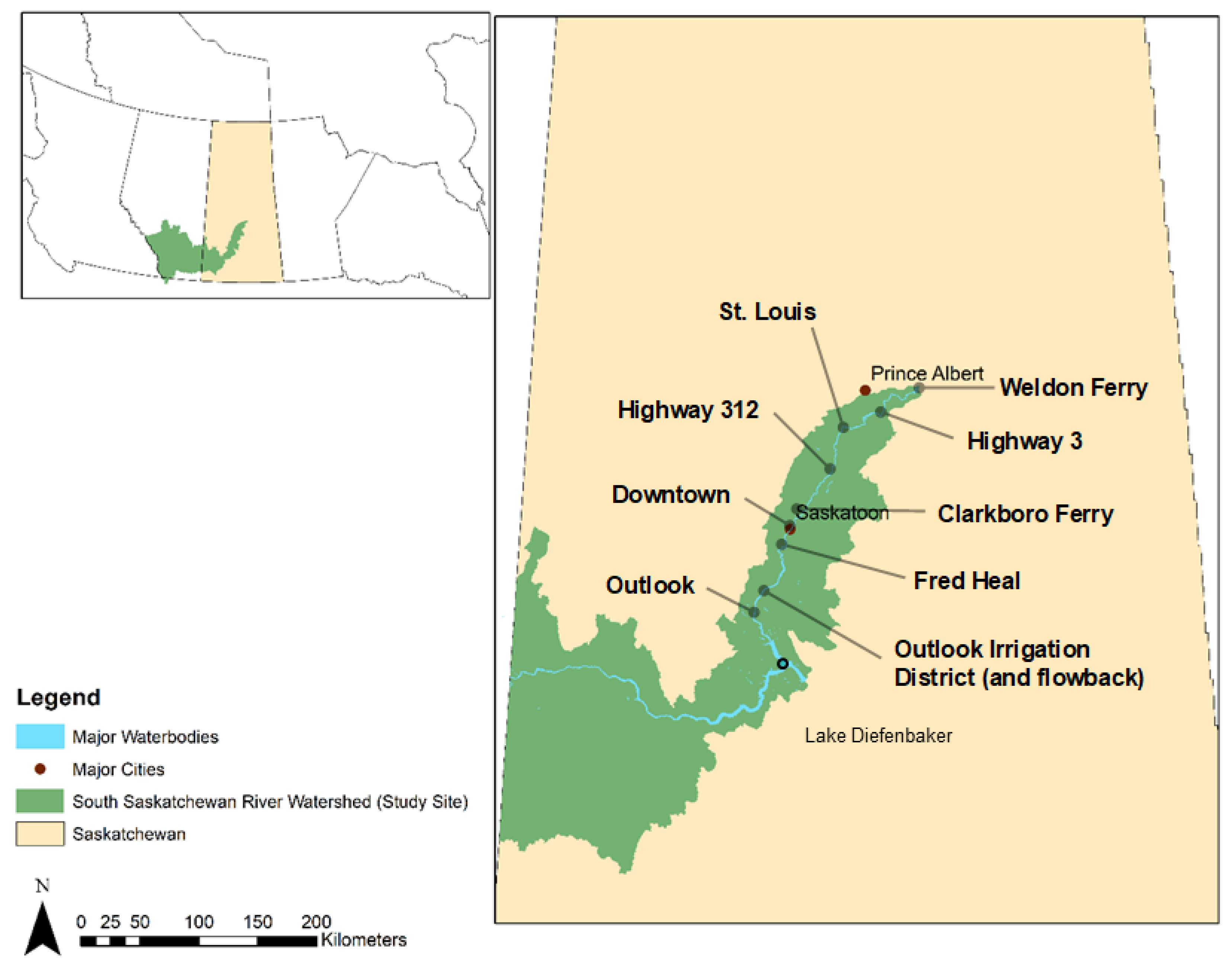
The Saskatchewan River system, which originates in Alberta’s Rocky Mountain headwaters and flows through Canada’s plains, is made up of the South and North Saskatchewan Rivers. The South Saskatchewan River Basin, which includes the major cities of Saskatoon, Swift Current, Red Deer, Calgary, Lethbridge, and Medicine Hat, is situated in the southern regions of Alberta and Saskatchewan (Figure 1). Big Stick Lake, Bow River, Oldman River, Red Deer River, Seven Persons Creek, South Saskatchewan River, and Swift Current Creek are all parts of the South Saskatchewan River Basin [28].

The Red Deer, Bow, and Oldman rivers meet at the confluence of the South Saskatchewan River, which is fed by the glaciers of the Rocky Mountains. From its source, the South Saskatchewan River flows for another 1392 kilometres. The SSR has an average discharge of 280 m³/s at the Saskatchewan River Forks. It covers a watershed of approximately 146,100 km², of which 1800 km² are in Montana, United States, and 144,300 km² are in Alberta and Saskatchewan [29]. Agriculture accounts for two-thirds of the land cover [30].

2.2. Modelling Approach

The change of heavy metals in the South Saskatchewan River system was studied using the Water Quality Analysis Simulation Program 7.52 (WASP) coupled with HEC-RAS. The WASP model could be used to simulate many different aquatic systems. The application could simulate hazardous water contamination using the concepts of mass, momentum, and the conservation of energy. The hydrodynamics of the model domain was simulated using the hydraulic model HEC-RAS 6.3. Since HEC-RAS was developed by the U.S. Army Corp of Engineers (USACE), all users and organizations have access to a free version of the model. HEC-RAS is available to everyone and does not require a license, making it a key benefit of utilizing it as a modelling tool. HEC-RAS can model flow, sediment transport, water quality in one-dimensional (1D) steady and unsteady flow, and two-dimensional (2D) unsteady flow of rivers. The model uses geometric data representation and geometric and hydraulic computer algorithms for a network of river channels. The HEC-RAS program can simulate an input flood using either a (1D) unsteady flow model or a (2D) unsteady flow model following these parameters.

Flow data were acquired from available flow data from the Water Survey of Canada (WSC) station at Lake Diefenbaker, which has an operational gauge (records available from 1966 to the present). That station is about 13 km upstream of the modelling upstream boundary (gauge 07DA001—South Saskatchewan River Below Lake Diefenbaker). The HEC-RAS model was calibrated by modifying Manning’s N to obtain the best match of the water level at 05HG001—South Saskatchewan River at Saskatoon and 05KD007—Saskatchewan River below the forks.

A 1D modelling approach was chosen as the optimum method for simulating the South Saskatchewan River sites. A 1D modelling approach was found to be reasonable for the region with optimum processing times. One-dimensional modelling can give results that are on par with, or better than, 2D models for rivers and floodplains where the predominant flow directions and forces follow the main river flow route, with less effort and fewer computing resources [31]. It was expected that the system was mixed both laterally and vertically. Previously, 1D WASP and HEC-RAS coupling [32] and quasi-2D [33,34] have been carried out.

HEC-RAS carried out the hydrodynamic part of the modelling, and the output of the HEC-RAS model was used as an input (for water depth at each segment) for the WASP model.

2.3. Setup for Water Quality Modelling

The water quality part of the study was modelled using the Water Quality Analysis Simulation Program (WASP 7.32). Due to some stability problems, the newer version of WASP was not considered for the current study. WASP was first created in the 1980s and has undergone numerous improvements [35]. The general dynamic model WASP uses a segmentation network to solve the conservation of momentum, energy, and mass equations and simulate the transport of contaminants and sediment. The WASP model is frequently utilized to address sediment transport [34], heavy metal transfer [33], and water quality issues [36,37]. The WASP stream transport module, TOXI, is coupled with flow routing for free-flow streams, ponded segments, and backwater reaches and is capable of calculating the flow of water, sediment, and dissolved constituents across branched and ponded segments. Additionally, model boundary constraints and input parameters are defined.

Water flows through a network of branching streams, which may contain both free-flowing and ponded parts, and is calculated using the standard WASP8 stream transport model. Flow routing can be estimated for free-flowing stream reaches, ponded reaches, and backwater or tidally-influenced reaches for one-dimensional branching streams or rivers. Advective transport can be driven through free-flowing portions with the simple yet practical kinematic wave flow routing method. The kinematic wave equation determines the propagation of flow waves and the fluctuations in flows, volumes, depths, and velocities that arise from the varied upstream inflow. This well-known equation is the solution to the one-dimensional continuity equation and a simplified form of the momentum equation that considers gravity and friction.

2.4. Kinematic Wave

For most simple river systems, the kinematic wave formulation is applicable. The kinematic wave calculates flow wave dissemination and flow velocity variations over a network of streams. The roughness of the slope and river bottom affect kinematic flow waves. By changing the Manning equation (Equation (1)) in the continuity equation and differentiating cross-sectional area with respect to time, the kinematic wave differential equation may be produced (Equation (2)).

$$Q=\frac{1}{n}\frac{A^{5/3}}{B^{2/3}}{S_0}^{1/2}$$

(1)

$$\frac{\partial Q}{\partial x}+\alpha \beta Q^{\beta -1}\frac{\partial Q}{\partial t}=0$$

(2)

where $Q$ is the flow rate, $x$ is longitudinal distance in channel, $t$ is time, $\alpha$ and $\beta$ are functions of hydraulic coefficients, $S_0$ is the slope of the channel, n is the Manning friction factor, A is the cross-sectional area, and B is the channel width. The depth exponent is used along with segment geometries to estimate hydraulic coefficients, which are later used to calculate segment flow depths under specific flow rates. [38] gave a complete description of WASP’s stream transport. To quantify variations in velocities, widths, and depths across the network, the kinematic wave based on solutions of one-dimensional continuity equations, and a condensed version of the momentum equation that takes the effects of friction and gravity into account, was utilized.

2.5. Discretization

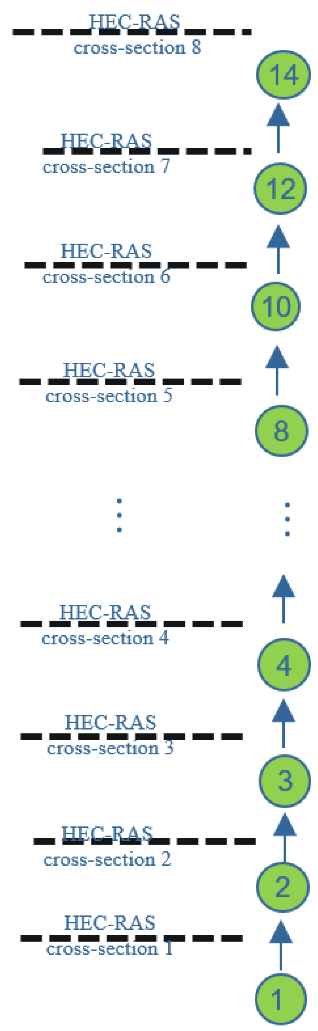
The river network was discretized using a 500 m interval. This led to 319 horizontal, one-dimensional water segments in WASP. Segment widths, average depths, and depth exponents were among the hydrodynamic metrics produced by HEC-RAS. The depth exponent controls channel shape in WASP. For these segments, a depth exponent value of 0.3 was used to simulate an uneven cross-section. Along with segment widths, slopes, and roughness factors, these depths are used in simulations to determine segment depths. The model’s input variables include channel geometry, flow routing, boundary conditions, environmental time functions, loads, and initial segment conditions. Hydraulic parameters were obtained using a calibrated and validated HEC-RAS model and utilized as inputs for the flow functions in WASP [38]. From the 319 HEC-RAS cross-sections separated by 500 m, geometry for the WASP segments (average depths, widths, and slopes) was derived. Based on the station’s water quality data closest to the study region, spatial linear interpolation was used to identify the boundary and initial conditions for the current investigation.

The study’s duration was from 2020 to 2021. Initial heavy metal concentrations for each model component were derived by interpolating between two nearby long-term monitoring stations: the upstream boundary conditions were defined using the nearest long-term heavy metal data, which was Outlook. The boundary data for downstream was used based on the data from Weldon Ferry.

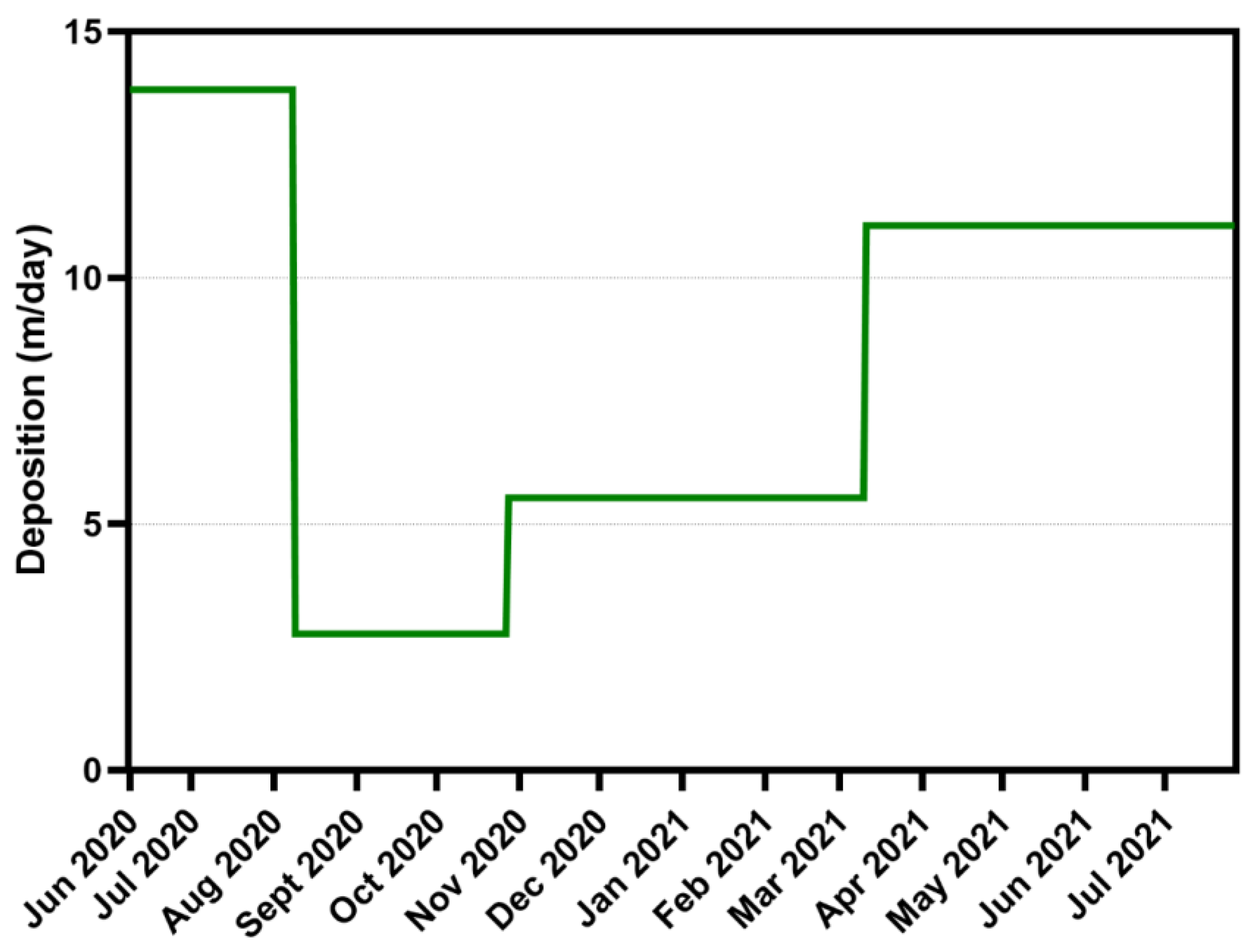
A segment length of 500 m was used for modelling. This length is deemed appropriate based on processing times, a reasonable uniform volume for segments, and an acceptable mixing. Benthic segments were inserted underneath each section of surface water to quantify erosion and sedimentation. The measured concentration at the upstream and downstream boundaries was used to calibrate the deposition rate of metals. In the HEC-RAS model, the spaces between each pair of cross-sections were split into individual WASP segments. Output files of the hydrodynamic model (HEC-RAS) were specific for each cross-section. These results then needed to be averaged between two consecutive cross-sections to obtain the exact values for each WASP segment. This procedure is shown in Figure 2 and was implemented in Microsoft Excel (Version 2211) for all input values.

2.6. Visualization, Calibration, and Validation

The modelled heavy metal concentrations and hydrodynamics were calibrated and validated. The calibration of heavy metal concentrations involved several iterations in the parameter space within reasonable parameters of the observed values. The best curve fitting with the observed data was achieved by choosing the optimum parameter values. To validate the model, a run with these values was compared against an independent set of field data.

An effective way to review model simulations and calibrate them using collected data is to utilize the post-processor (MOVEM). Results from every WASP run, as well as others, can be visualized using MOVEM. MOVEM allows the modeller the choice of two graphical representations of the results: geometric grid and x/y plots. There is no restriction on how many geographical grids, x/y plots, or even model result files a user can employ in a session.

3. Results

3.1. Deposition Rates and Overall Concentration Trends

First, it was assumed that the deposition rate for copper and nickel should be the same as sediment. Deposition rates for copper and nickel were calibrated using the sampled concentration at the upstream and downstream model boundaries (Figure 3). A previously developed model for sediment transport was used, and the model was calibrated with an acceptable range of deposition [38]. Concentration plots (Figure 4) show the trend for both trace metals at selected sampling sites (Downtown, Clarkboro Ferry, and Highway 312) for both water and sediment samples. Concentration values for all sites can be found in the Supplementary Information.

Both trace metals were modelled for the same time periods for water and sediment in the years 2020 and 2021 and matched to the field sampling of water and sediment samples to maintain uniformity.

3.2. Copper

In 2020, copper concentrations were observed in the range of 1–5 µg/L except for two sites (Highway 3 and Weldon Ferry), with values at 42.2 µg/L and 20.2 µg/L, respectively (refer to Supplementary Information). Cu concentrations in river water in 2021 were in the range of 0.8 µg/L to 5 µg/L. That the observed concentrations remained uniform, for the most part, is indicative of the complex mixing of copper across the sampling sites, whereas elevated concentrations of copper at Highway 3 and Weldon Ferry could be attributed to various constructions around the location (bridges and roadway) in this area (S. Prajapati, pers. obs.). Many of the measured concentrations were over the long-term CCME water quality guideline for Cu of 4 µg/L at the given water hardness > 180 mg/L CaCO₃, which indicates that risks to aquatic life could not be excluded. Sediment Cu concentrations ranged from <LOQ to 19 mg/kg in 2020 and <LOQ to 15 mg/kg in 2021 [27]. Since the resulting concentrations are below the CCME ISQG of 35.7 mg/kg, the authors do not expect adverse effects. In sediments, Cu ranged from 1–15 mg/kg, with Clarkboro Ferry being on the higher end for both sampling years, with values in the range of 12–15 mg/kg.

Figure 5 and Figure 6 show a longitudinal comparison of measured and modelled copper concentrations in water and sediment for 2020 and 2021. The concentrations modelled through the sampling time points almost uniformly increased between the upstream and downstream boundaries of the study area. Copper concentrations for water samples remained mostly consistent for June 2020, August 2020, and October 2020, but increased gradually and became more consistent in June 2021 and August 2021. Within the study period, discharge and flow velocity of the South Saskatchewan River were highest in June 2020, which can explain this observed pattern of copper concentrations, as increased discharge would cause significant erosion of riverbanks and stream beds. Thereafter, longitudinal profiles for August 2020, October 2020, and June 2021 remained relatively consistent throughout the segments.

3.3. Nickel

In 2020, nickel concentrations ranged consistently from 2–6 µg/L for water samples and ranged from 0.3–1.4 µg/L in 2021. The high-flow season in 2020 (due to elevated discharge and precipitation mentioned above) helps explain the almost three- to fourfold greater nickel concentrations in that year. Levels of nickel in sediments for 2020 ranged from 10.5–25 mg/kg and mostly remained consistent throughout the year. However, in contrast to concentration values for water samples, the concentration of nickel in 2021 remained around the same range, with a very slight decrease, ranging from 10–20 mg/kg. No measured values were observed to be over the long-term CCME water quality guidelines for Ni of 150 µg/L at the given water hardness > 180 mg/L CaCO₃.

Longitudinal profiles for nickel (Figure 5 and Figure 6) followed almost the same trend as those for copper, with very little variability in concentration values during the different sampling time points. Nickel concentrations remained consistent for August 2020, October 2020, June 2021, and August 2021, with a slight gradual increment with every major segment (i.e., sampling station). The concentration values followed a similar trend of gradual increase. For sediment samples, the modelled progressions again followed similar patterns in August 2020, October 2020, and June 2021, with a consistent and slight decline throughout the study area. Again, high flow in 2020 could explain the three- to fourfold greater nickel concentrations in 2020 compared to 2021 water samples. Similarly, for sediment samples, settling and transverse mixing can contribute to consistent and slight declines in the concentration values.

4. Discussion

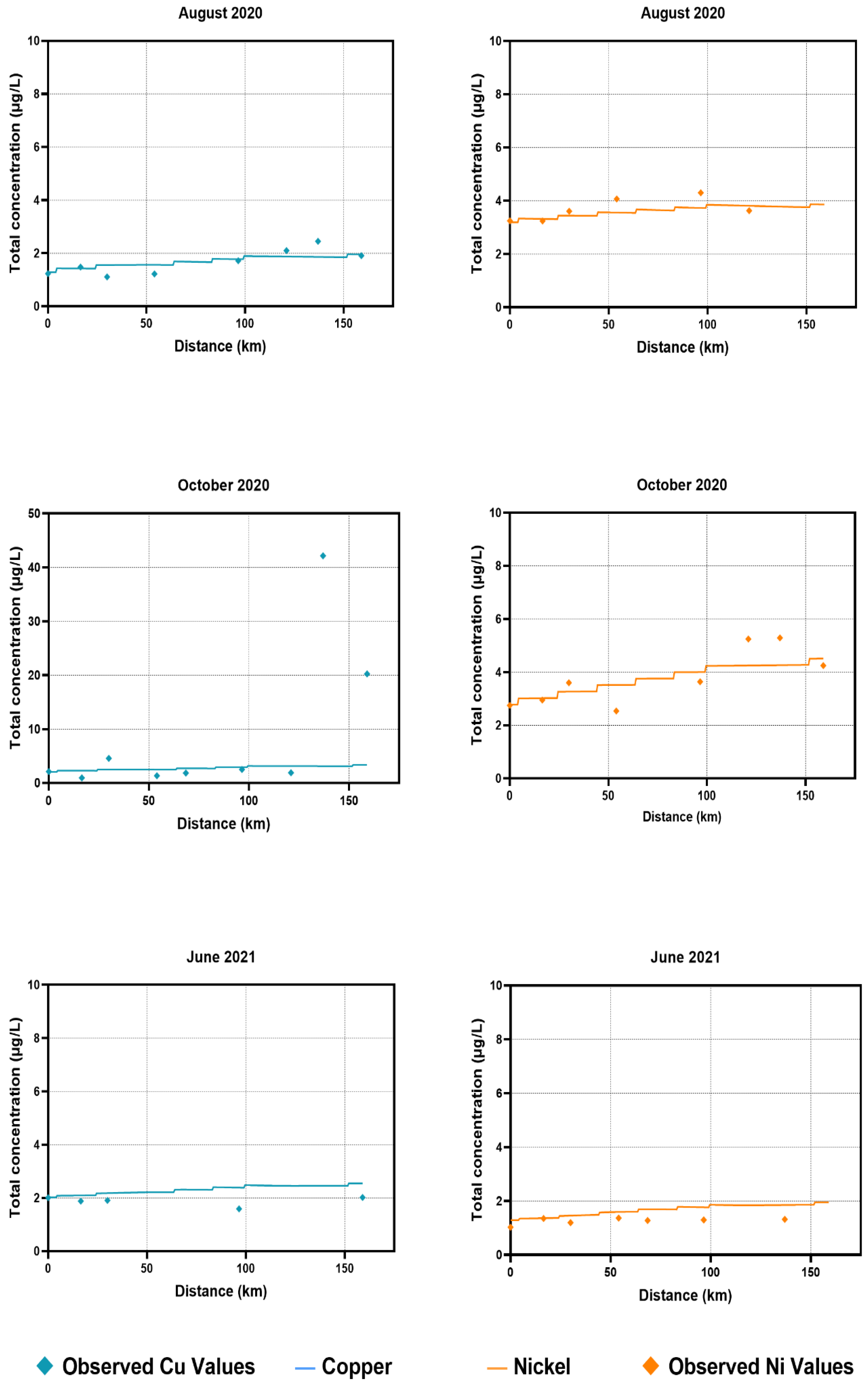
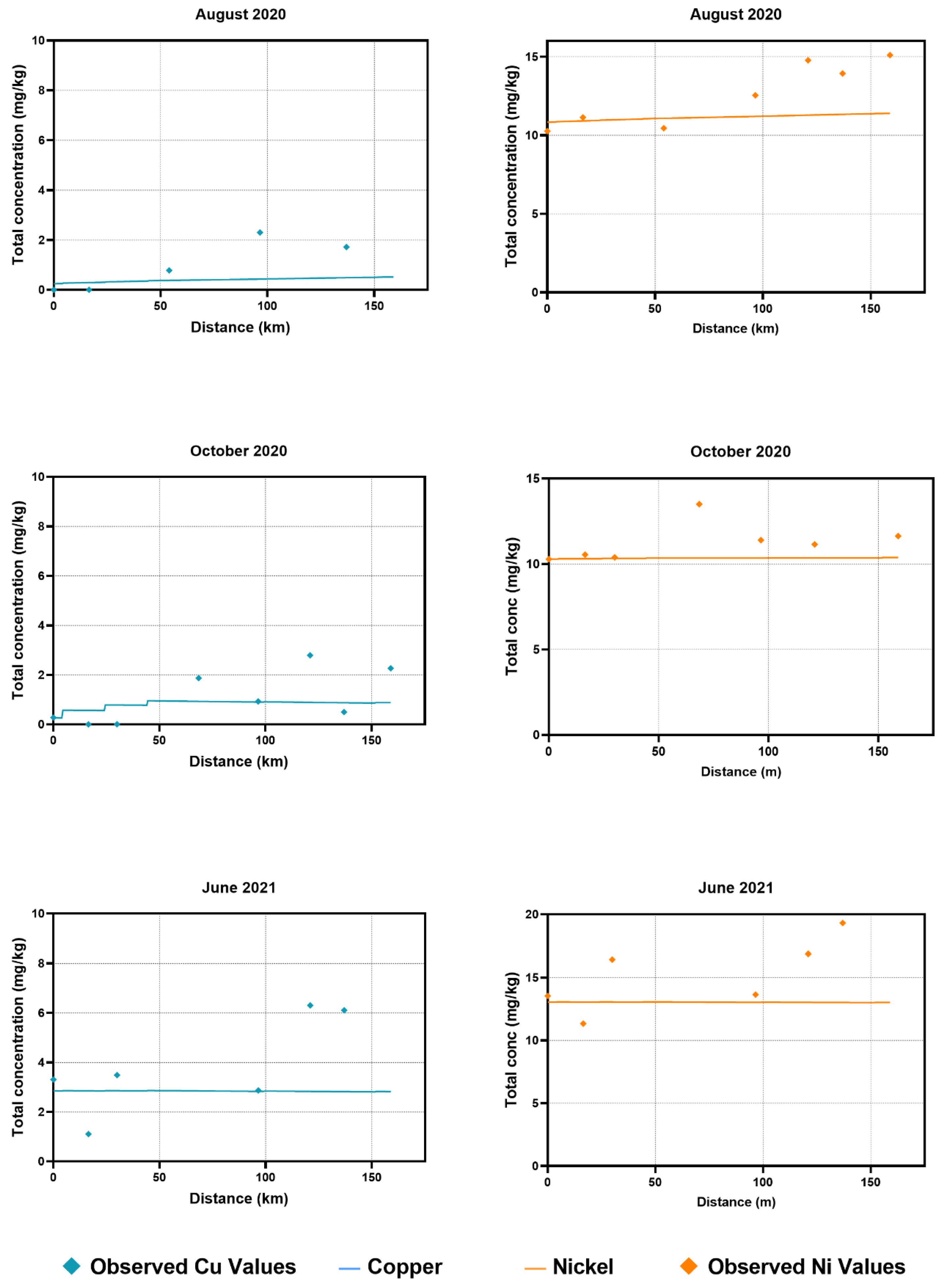
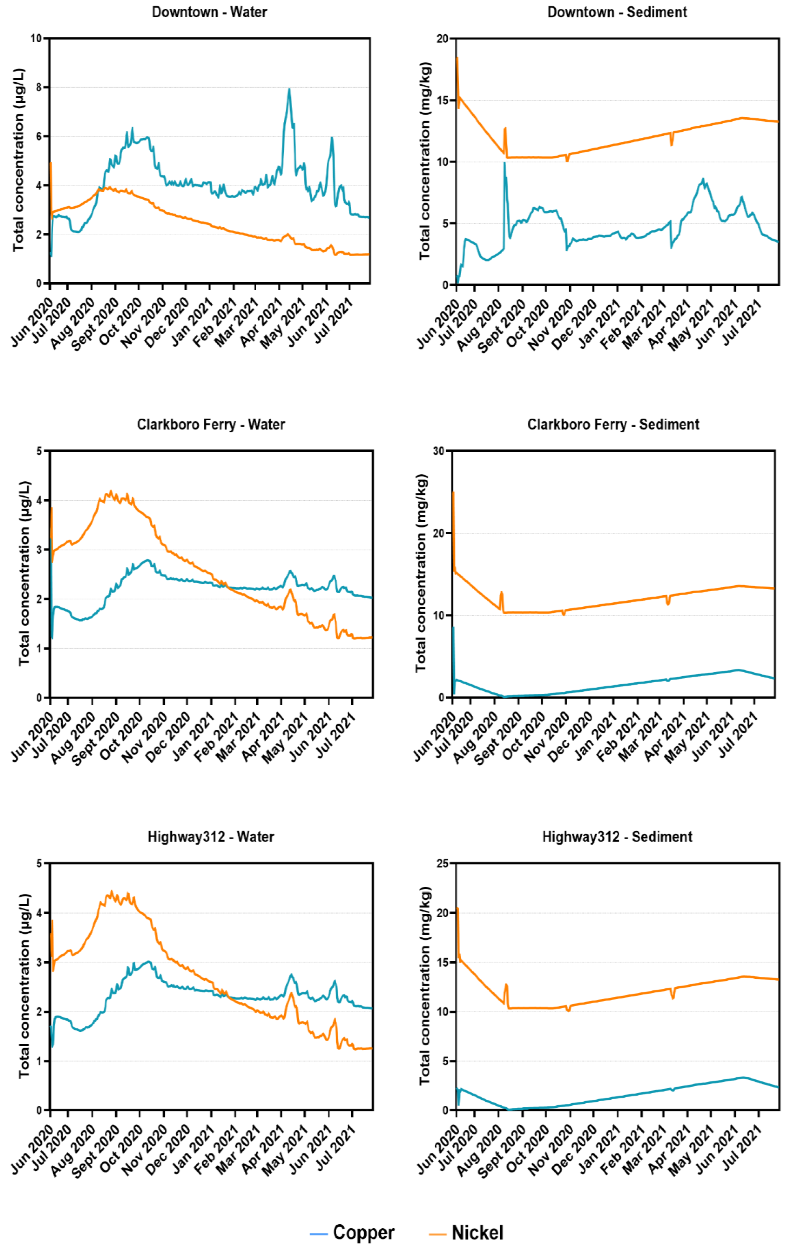
Observed copper concentrations in water were consistent and followed similar trends to the observed values for most of the sampling time points. An exception to that is the observed values in the October 2020 sampling time points, where the copper concentration values were significantly higher than that of the trend following the WASP simulated values. This could be attributed to roadwork and bridge construction in the area, which would have been impossible for the model to cover. In sediment samples, the majority of the WASP simulated values were underestimated compared to the observed values, with a few exceptions. This could be the result of the continuous accumulation of metals in sediments over many years, which was not accounted for in the current modelling exercise.

Modelled nickel concentrations in water samples across 2020 and 2021 also followed a similar trend, without major discrepancies from the observed values. For sediment samples, there were a few instances where the observed values were higher than those of the modelled progression. The model tended to underestimate the nickel concentrations for sediment samples, following a similar trend to the copper concentrations for sediment samples.

During simulations, the model was found to be underestimating the concentrations at downstream segments. Additional diffuse loads were added to compensate for matching the simulated values with measured values. This significantly improved the accuracy for both metals. For water samples, additional loads (~1–3 kg/day) were included at major segments (sampling stations) as diffuse loads. The loads were increased 100-fold for the calibration of sediment samples. Calibration process determined these amounts. Copper and nickel are both known to sequester in the sediment bed and are less likely to be suspended in water. Copper, as mentioned above, enters the environment mainly through anthropogenic sources [4]. The release and remobilization of sediment-bound copper have been well-documented in various studies; however, the overall impacts are minor [39,40]. Mobility of nickel, on the other hand, is site-specific and depends on the soil type and pH [41]. These observations can be attributed to the higher observed values of nickel and copper in the sediment samples in the current study.

The model used in the current study is an extension of the previously developed model 1D WASP and HEC-RAS coupling [32] and quasi-2D [33,34]. In the study [38], the mixing of vanadium and sediment was modelled with a quasi-2D modelling approach in the lower Athabasca River. The authors observed a marked increase in vanadium concentration along the river. The model was successful in capturing the transverse mixing from tributary water with mainstream water.

As mentioned earlier, modelling freshwater systems is challenging, involving many complex processes that affect contaminants’ transport and fate [42], which demands sensitive methods to obtain accurate results for different metals. With limited data availability, understanding metal speciation becomes difficult in such systems [43]. The current study for the South Saskatchewan River system serves as a preliminary study focusing on trace metal transport and fate. This study also provides an understanding of how the concentrations of trace metals (Cu and Ni) vary across upstream and downstream of the South Saskatchewan River. There were a few CCME ISQG exceedances for Cu concentrations, and there are no guidelines outlined for Ni (as of now). Although there may be no immediate danger just yet, contamination of aquatic systems cannot be excluded. Further study involving more metals in the model with sufficient input parameters would be an ideal recommendation.

5. Conclusions

The aim of this study was to better understand trace metal fate and interaction in the South Saskatchewan River. Two trace metals, copper (Cu) and nickel (Ni), were selected on the basis of their presence in the region. Copper is used in a wide range of products such as construction, pipes, industrial equipment, etc., resulting in widespread anthropogenic contamination with Cu. In contrast, nickel has a geogenic background in Saskatchewan and is transferred to the aquatic environment by effluents, leachates, and runoff from mining activities and the general land surface.

A 1D modelling approach was successfully applied in studying the trends and patterns of trace metal fate in the river and sediment. The simulations provided interesting data for both the trace metals and gave an insight into how the metals travel and react between water and sediment in the South Saskatchewan River.

A number of parameters needed to be assumed due to the lack of availability of consistent raw data for the modelling of these two trace metals. Improved availability of these parameter values would help make the model more efficient and accurate in predicting future trends with increased/decreased flows.