Article

Deep Learning Approach with LSTM for Daily Streamflow Prediction in a Semi-Arid Area: A Case Study of Oum Er-Rbia River Basin, Morocco

1
Data4Earth Laboratory, Faculty of Sciences and Technics, Sultan Moulay Slimane University, Beni Mellal 23000, Morocco
2
Centre for Remote Sensing Applications (CRSA), Mohammed VI Polytechnic University, Ben Guerir, Green City 43150, Morocco
3
International Water Research Institute (IWRI), Mohammed VI Polytechnic University, Ben Guerir, Green City 43150, Morocco
*
Author to whom correspondence should be addressed.
Water 2023, 15(2), 262; https://doi.org/10.3390/w15020262
Submission received: 3 November 2022 / Revised: 26 December 2022 / Accepted: 4 January 2023 / Published: 8 January 2023
(This article belongs to the Section Water Resources Management, Policy and Governance)

Abstract

:
Daily hydrological modelling is among the most challenging tasks in water resource management, particularly in terms of streamflow prediction in semi-arid areas. Various methods were applied in order to deal with this complex phenomenon, but recently data-driven models have taken a better space, given their ability to solve prediction problems in time series. In this study, we have employed the Long Short-Term Memory (LSTM) network to simulate the daily streamflow over the Ait Ouchene watershed (AIO) in the Oum Er-Rbia river basin in Morocco, based on a temporal sequence of in situ and remotely sensed hydroclimatic data ranging from 2001 to 2010. The analysis adopted in this work is based on three-dimension input required by the LSTM model (1); the input samples used three splitting approaches: 70% of the dataset as training, splitting the data considering the hydrological year and the cross-validation method; (2) the sequence length; (3) and the input features using two different scenarios. The prediction results demonstrate that the LSTM performs poorly using the default data input scenario, whereas the best results during the testing were found in a sequence length of 30 days using approach 3 (R2 = 0.58). In addition, the LSTM fed with the lagged data input scenario using the Forward Feature Selection (FFS) method provides high performance accuracy using approach 2 (R2 = 0.84) in a sequence length of 20 days. Eventually, in applications related to water resources management where data are limited, the use of the deep learning technique is able to create high predictive accuracy, which can be enhanced with the right combination subset of features by using FFS.

1. Introduction

Water resources are of great importance to ensure the world’s needs, including for agriculture, industrial and domestic usage, as well as for other environmental systems. However, the availability of water resources is being limited in many countries around the world, especially in arid and semi-arid regions due to climate change, population increase, and irrigation expansion that affects socio-economic development and food security. In Southern Mediterranean regions, the degree of water scarcity and drought conditions may also increase the pressure on water resources [1,2]. In addition, these areas are characterized by low precipitation with irregular spatiotemporally distribution and high evaporation. This controls the streamflow process that present a paramount component for understanding and monitoring the quality and quantity of the water supply [3,4]. Therefore, improving streamflow prediction in arid and semi-arid regions is a challenging task for sustainable water resources management and watershed planning, because it has provided valuable statistics to decision-makers for the assignment of accessible water for different purposes, particularly for the agriculture sector [5]. This is the case in the Oum Er-Rbia river basin, which serves as one of the heartbeats of hydroelectric and irrigation networks in the kingdom [6]. Successful and efficient water resources management require accurate and timely streamflow information. In this context, numerous methods have been used to estimate the streamflow at gauged or poorly gauged watershed involving empirical, physical, conceptual, and data-driven methods [7]. Empirical models rely only on the information based on existing data, without taking into account the characteristics of hydrological processes [8]. Physical and conceptual models may be two of the best hydrological models to simulate streamflow [9], but they need considerable parameters and require more effort to construct [10]. Therefore, data-driven approaches, including machine learning and deep learning, have been revolutionary tools in the watershed planning process. They have largely improved streamflow simulation with no requirement of physical and underlying processes [11].
For machine learning, Support Vector Machine (SVM), regression trees and Artificial Neural Networks (ANNs) are the popular tools utilized to build prediction models, which have definitely improved their ability to solve regression issues [12,13]. For streamflow simulation, several studies have been carried out to thoroughly evaluate the methods mentioned. For example, Hadi and Tombul [14] indicated that ANN performs better than SVM to predict streamflow on a daily scale with different physical characteristics. On the other hand, Parisouj et al. [15] revealed that machine learning models achieve favorable performance, especially the SVR, in a daily and monthly time step in different climatic zones. Besides, the reason behind the higher accuracy in each model is due to the input feature and training data, or to the model structure that can affect the selection of the accurate one. Indeed, traditional machine learning algorithms have a simple structure and less data requirement, but ANN and SVR are quite inefficient to capture the series’ information in the input data, which is required for handling with the sequence variable [16].
To overcome the potential limitations of machine learning techniques, the use of deep learning, particularly for time series data, provides higher accuracy [17]. Deep learning is a growing field with various studies that have been performed for time-series predictions. Recently, one of the famous models used in this field is the Recurrent Neural Networks (RNNs), considering the structure of RNN networks which has a solid aspect of sequence architecture that allowed information to preserve [18]. However, because of its structure, this neural network’s computation is slow and difficult to process long sequences, and it is incapable of dealing with the vanishing gradient challenge. Long-Short-Term-Memory (LSTM), a powerful RNN architecture, was developed to address vanishing gradient issues [19]. Due to such capacity, LSTM has been applied by many researchers for streamflow prediction, as the streamflow information is associated with the last values over extended periods of time [20,21,22]. Apaydin et al. [23] indicated that LSTM gives a better performance with supportive accuracy that make them useful for streamflow modeling, compared to ANN and simple RNN models that show an inferior reaction. Nonetheless, there is a difference between simulating streamflow within a daily and monthly time extent. The LSTM model is more applicable for daily prediction, while for monthly modeling ANN got the most accurate results. For example, Cheng et al. [24] found that, compared to ANN, the LSTM model displays a better results performance in daily prediction and less accuracy in a monthly scale because of the absence of an extensive monthly training dataset. Both approaches, ANN and LSTM have diverse scenarios, but they are similar and have advantages that make the long and short predictions more powerful predictive and effective, but with a priority to LSTM [25]. The quantity of hydrological and meteorological data plays a critical role in predicting streamflow, as long as the improvement of the higher potential model is related to the higher aspect of the data [26]. Several studies noted the effect of feeding the LSTM model with various meteorological data conditions on the performance of the model [27] through the streamflow process. For example, Choi et al. [28] successfully adopted the LSTM network to evaluate the composition of input variables on a daily scale. Moreover, due to the luck of management, the observed data may be disordered and insufficient for training the model, which affects the LSTM efficiency. However, the implantation of the LSTM model on a gauged or poorly gauged river basin seems reliable due to the training data that presents the backbone of the LSTM structure [29]. Coi et al. [30] demonstrate the ability of the LSTM model to predict streamflow without hydrological observations. The findings revealed that the model is highly depending on the amount of available data. Therefore, recent methods focus on overcoming the problem by proposing different inputs. Kieran et al. [31] trained the LSTM model to predict streamflow using hydrological and meteorological satellite data as well as the antecedent observations of streamflow. Similarly, Rahimzad et al. [32] explored the capabilities of LSTM compared with different data-driven techniques based on historical streamflow and precipitation time series. The results revealed that the LSTM model is a robust network to distinguish sequential data series behaviors in streamflow modeling.
Furthermore, the input data of LSTM requires a three-dimensional array as an input: input samples, sequence length, and input features. The relationship between the input features and the sequence length may have influences on model performance, as the third dimension represents the number of features in the input sequence considering the previous time steps as input variables [33]. The impact of sequence length with the input data on the streamflow prediction performance needs to be developed.
Although there are studies that aim to solve hydrologic problems in Morocco, such as in Berrchid city where machine learning models were used to forecast groundwater quality [34], but there are scarcely any studies that evaluate streamflow prediction using deep learning techniques. Thus, we found it to be a new debate area and interesting task to work on.
The designed experiments in this study will focus on evaluating the reliability of the LSMT network to simulate daily streamflow in a semi-arid mountainous watershed in Morocco, using meteorological data and remotely sensed information. However, the importance of the LSTM model can take advantage of information among time-series data, and performs better in predicting streamflow variability that represent a tendency over time. Thus, in order to elucidate the significance of the LSTM model in streamflow prediction, we explore the capability of the model within the time splitting zone using different approaches, as well as the effect of sequence length selection in the model performance. Moreover, due to the lack of data, this study also evaluates the impact of antecedent values of streamflow by comparing the performance of the model with two different forms of inputs. In the first instance, we initially presented the study area and the data used. This is followed by describing the model architecture and the methodology used. The last section is about the discussion of the training validation and testing results of different approaches that experiment with the effect of sequence length and input features in the LSTM’s performance of daily streamflow prediction.

2. Materials and Methods

2.1. Case Study

Oued El Abid is the largest affluent basin of the Oum Er-Rbia river, with an area of 7975 km2 located in the center of Morocco between the meridians 6°15′ W and 6°30′ W, and the parallels 32° N and 32°5′ N. This basin is a mountainous area with a significant water resource potential, feeding the Bin El Ouidane dam to cover the agriculture activities [35] and refreshing the groundwater downstream of Tadla plain [36]. This study area, as a typical South Mediterranean basin, is characterized by a semi-arid climate with an average of approximately 480 mm/year as well as strong spatiotemporal variations in precipitation. Western movements and orographic effects play a crucial role to generate rainfall. The rainy period of the year lasts for 6 months (November to April) and the dry period lasts 4 months (June to September) with a start of watering in October, a maximum in January, and a minimum in July. Depending on the high altitude of the Atlas Mountains and a yearly scale volume primarily accumulated during the spring season, which corresponds to the snowmelt, the flow gradually shifts from rain to snow. The variation of temperature is notably influenced by the high elevation involving snow occurrence. The temperature drops to −9 °C in the winter and rises to 41 °C in the summer [9]. The Oued El Abid river is made up of two main sub-basins, the sub-basin of Ait Ouchene and that of Teleguide. Our study focuses on the Ait Ouchene watershed (Figure 1, Table 1).

2.2. Data

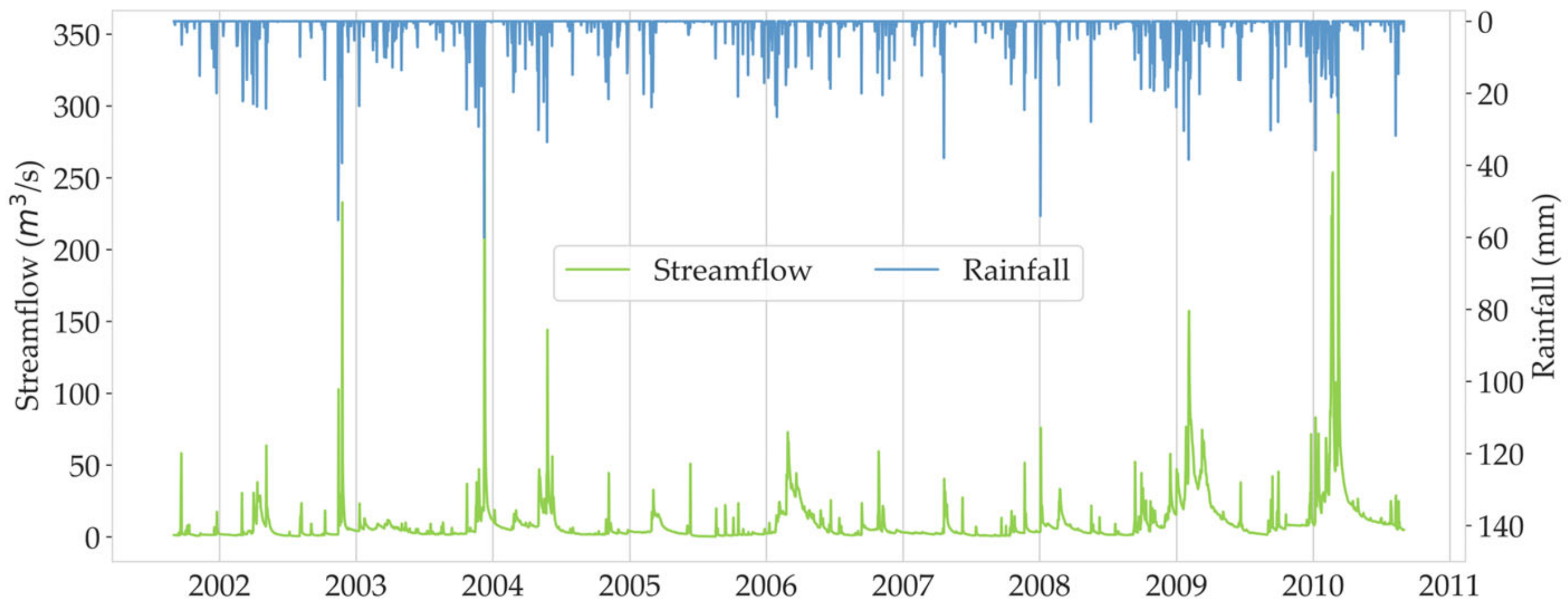
The simulation of streamflow requires timely datasets. In this study, daily hydroclimatic datasets (rainfall, streamflow, temperature, and snow cover area) from 2001 to 2010 were used: In situ observations of streamflow and rainfall were provided by the Oum Er-Rbia hydraulic Basin Agency (ABHOER) [37]. The regional rainfall of the Ait Ouchene watershed was represented by the average from the gauges situated within the same subbasin. The variation of daily measured streamflow and daily rainfall values is shown below (Figure 2). Due to the lack of ground measurement of snow depth, remote sensing was the main solution to estimate snow occurrence, especially over large mountainous basins. The daily snow cover time series (SCA) at a spatial resolution of 500 m were available from the National Snow and Ice Data Center (NSIDC) using Terra/MODIS (Moderate-Resolution Imaging Spectroradiometer) satellite data, MOD10A1 version 6 [38,39]. MODIS was chosen as a baseline for producing SCA, because it is reliable and provides a good streamflow simulation, according to Ouatiki et al., and it has been already studied and tested in many basins [9,32,33]. Additionally, the lapse rate approach was used to generate the daily temperature data at a rate of 0.56 °C per 100 m of elevation. [40].

2.3. Long Short-Term Memory (LSTM)

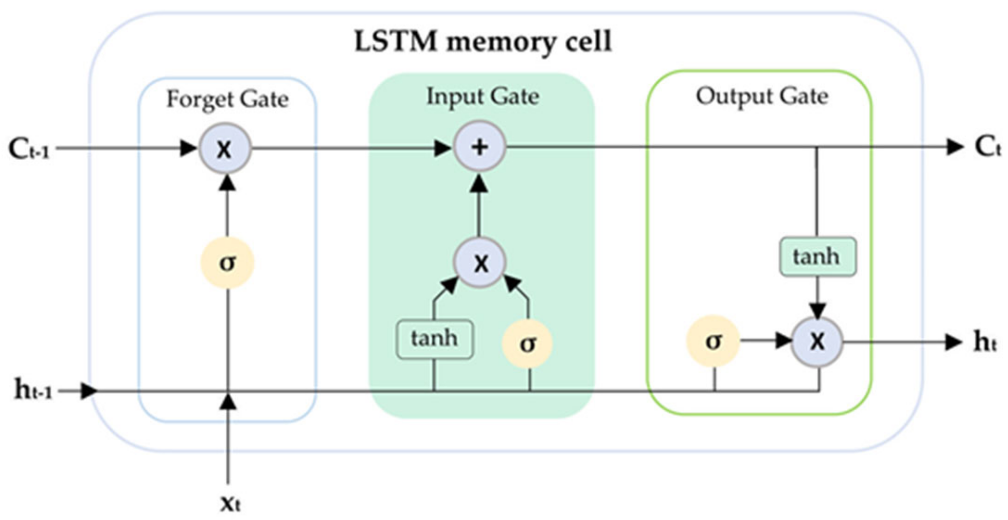
LSTM network is a particular variety of recurrent neural networks (RNNs) that was developed by Hochreiter et al. [19], and has been applied by many researchers due to the specific design that overcomes the long-term dependency problem faced by RNNs. [41]. The structure of LSTM depends on three basic conditions: the cell state that defines the current long-term memory of the network, the output at the prior point known as the hidden state, and the input data in the current time step [42]. Thus, the architecture of LSTM can control how the information in a sequence of data comes through three special gates: the forget gate, the input gate, and the output gate (Figure 3).
The first step in the process is the forget gate (Equation (1)). The decision is taken through a sigmoid layer. Then, the input gate (Equation (2)) determines what value should be added to the cell state, taking into account the previous hidden state and the new input data. This step has two parts: the input gate layer that decides which values will update, and the tanh layer (Equation (3)). The previous cell state Ct-1 is then updated into the new cell state by combining the two layers (Equation (4)). The output gate (Equation (5)), which determines the new hidden state, is the last phase. To decide which components of the cell state should be generated, it is important to run the sigmoid layer (Equation (6)). The mathematical formulas of the model structure are:
f t = σ W f h t 1 , x t + b f
i t = σ W i h t 1 , x t + b i
C ˜ t = tan h W c h t 1 , x t + b c
C t = f t ×   C t 1 + i t × C ˜ t
o t = σ W o h t 1 , x t + b o
h t = o t × tanh ( C t )

2.4. Methodology

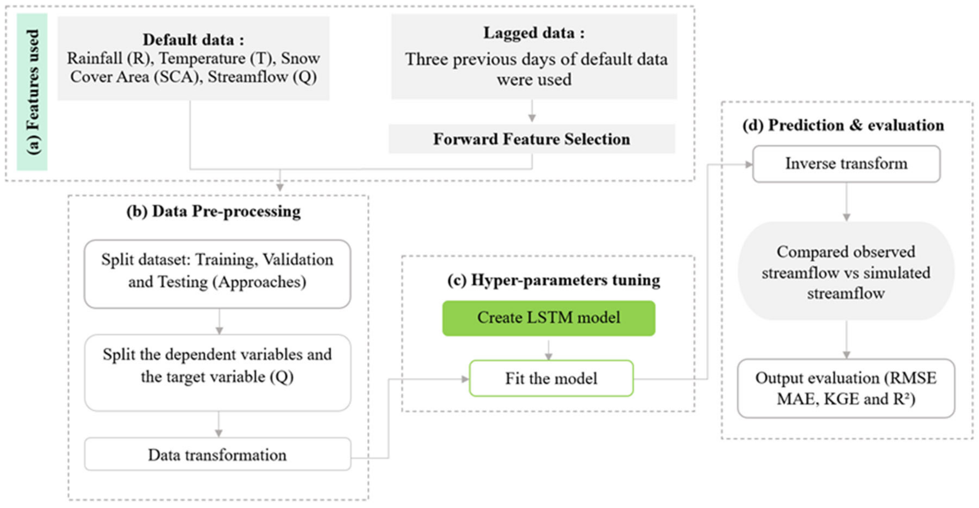
The Python-based TensorFlow open-source software package and Keras were used to create the LSTM model for this study. The process used is illustrated in Figure 4, and is divided into four main steps: feature selection (a), data pre-processing (b), hyper-parameters tuning (c), prediction and evaluation (d).

2.4.1. Feature Selection

In this study, we created two input scenarios to explore the sensitivity of the LSTM model in this region. First, rainfall (R), temperature (T), and snow cover area are (SCA) used as default inputs (scenario 1: LSTM). The second input scenario was generated by adding lagged data, conditions, and information on indicators providing the historical point of reference for the next steps. Thus, it will be used to assess the achievement of the effect and outcomes expressed in the model. The number of time lags of the streamflow was determined by using the Partial Autocorrelation Function (PACF) [43]. Days 1, 2, and 3 were significant and had an impact on the streamflow at t = 1 day. Three lag days of rainfall, temperature, and SCA were considered to select the model features. However, to find the best subset of features, we used the Forward Feature Selection (FFS) algorithm [44], which evaluates each individual feature by incrementally adding the most relevant ones to the target variable (streamflow) [45]. The subset of features that were found to be significantly correlated with the streamflow are presented in Table 2 (scenario 2: FFS-LSTM).

2.4.2. Data Pre-Processing

This study identified additional concerns regarding the accuracy and reliability of the LSTM model. Accordingly, it is typical to have a mechanism to evaluate the overall performance of the model. Thus, splitting the input data into training (train LSTM) validation (evaluate LSTM) and testing (confirm the results) is the apparent and fast procedure to limit the model from overfitting and to compare its effectiveness in streamflow prediction. Although with time-series data, it is crucial to consider the back values that will be used for testing and training [24], hence we split the data using three approaches:
  • Approach 1: splitting data to 70% training, 15% validation, and 15% testing [5,25]. The learning period was set from 1 September 2001 to 14 December 2007, the validation period was from 15 December 2007 to 24 April 2009, and the testing period was from 25 April 2009 to 31 August 2010.
  • Approach 2: splitting data taking into consideration the hydrological year that started from September of the current year and ended in August. Six years for training (1 September 2001–31 August 2007), one year and 6 months for validation (1 September 2007–28 February 2009), and one year and 6 months for testing (1 March 2009–31 August 2010).
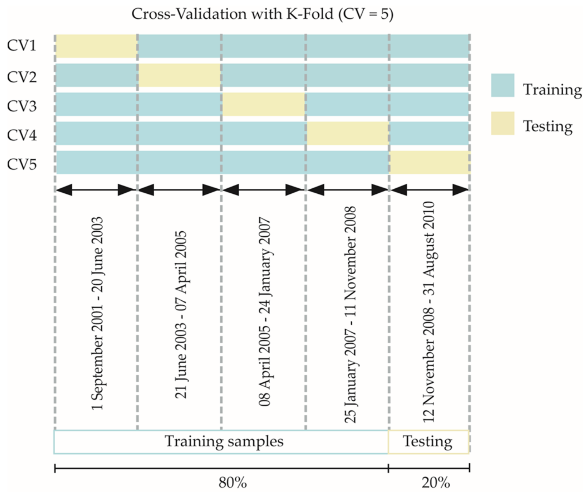
  • Approach 3: with limited data samples, k-fold cross-validation is the most widely used method to assess the model’s performance. It divides the dataset in k equal-sized numbers, with one out of k parts is used as the testing set while the model is trained using k-1 folds [43]. The configuration of the cross-validation parameter is referred as the number of split iterations that the dataset will be divided into. Overall, it is from 2 to 10 depending on the availability of the data. In this study, we tested the different values of cross-validation (CV). The appropriate value is CV = 5 with 80% as the training set (7 years), along with 20% of the train data as the validation set and 20% for testing (2 years) in each group that was employed (Figure 5).
In addition, we separated the target variable (streamflow) and the input variables (rainfall, snow cover area, and temperature) from the dataset. The last step in the pre-processing action is the data transformation that plays a critical role in the performance of neural network models, when features are on a relatively similar scale and are close to being normally distributed. One of the most popular methods for scaling numerical data is normalization, which scales the input variables to a standard range between zero and one [46], and uses the same range for scaling the output corresponding to the activation function’s size (tanh) on the output layer of LSTM. The MinMaxScaler function (Equation (7)), was used to decrease the minimum values in the feature and divided by range using the original training data. It is important to estimate the minimum and maximum available values, and accordingly apply the scale to the training validation and testing. This estimation method scales and converts each feature individually, so that it falls within the training set’s given range of zero to one.
  x = x min x max x min x
where x’ is the scaled value, and x is the original value.

2.4.3. Hyper-Parameter Tuning

The configuration of the neural networks is still difficult because there is no strong and specific approach to develop the algorithm [47]. This is why we need to explore different configurations to decide and selected the values of parameters that can be used to control the learning process and avoid overfitting [42,44]. In general, neural networks have numerous hyperparameters that minimize the loss function. The LSTM parameters used in this study are composed of three neural network layers: the input layer, the hidden layer and the output layer. Moreover, we used a regularization method named dropout to reduce overfitting and improve the model performance. For the baches, we used 32 batch for the first scenario and 10 batch for the second scenario. The number of epochs used in this study is 250 epochs, with an early stop of 10 epochs when the model performance stops improving on the validation set. The hyper-parameters selected for the model are summarized in Table 3 [48,49].
Therefore, the architecture of the LSTM model is a 3D input (num_samples, num_timesteps, num_features) [50]. In this study, the number of sequence lengths was evaluated using five-time steps: 2, 10, 20, 25 and 30 (denoted TS2, TS10, TS20, TS25, TS30) days of input data employed to drive the LSTM network to predict to next day.

2.4.4. Model Evaluation Criteria

Typically, there are various criteria for evaluating model performance for streamflow prediction. In deep learning, these parameters serve to compare the difference between the observed streamflow and the simulated output from the validation and testing values. In our study, we evaluated the LSTM performance by employing the Root Mean Squared Error (RMSE, Equation (8)), the Mean Absolute Error (MAE, Equation (9)), the Kling-Gupta Efficiency (KGE, Equation (10)), and the coefficient of determination (R2, Equation (11)).
The most often used metric in prediction and regression tasks is the Root-mean-square deviation. RMSE is the average squared difference between the true values and the predicted scores. Here, y i (m3/s) presents the observed streamflow for each data point, and y i (m3/s) presents the predicted value. The range of values for RMSE is 0 to ∞, and a great prediction result is obtained when RMSE = 0 [51].
RMSE = i = 1 n y i y i 2 n
MAE is a popular metric defined by the units of the error score that corresponds to the units of the predicted value, and is calculated as the average of the absolute error values of the difference. The MAE does not give more or less weight to different types of errors, and instead the scores increase linearly with error increases. The value of MAE ranges from 0 to ±∞, When MAE = 0 the prediction result is the best. |yiyi| is the difference between the observed and expected values in absolute terms [52].
MAE = i = 1 n y i y i n
The Kling-Gupta Efficiency, KGE forward certain weaknesses in NSE and is increasingly utilized to calibrate and validate models. It was originally developed to compare predicted and observed time series which can be decomposed into the contribution of average, variance and correlation to model performance. Similarly to the NSE, when the optimal score of KGE = 1 the simulations and observations has a perfect match [53]. Different researchers use positive KGE values as indicators for “good” model simulations, whereas negative KGE values are regarded as ‘poor’. However, KGE = 0 is implicitly used as the dividing line between “good” and “poor” performance. In KGE, r is the Pearson correlation coefficient between actual and simulations values, β a result of dividing the simulation mean by the observation mean [33,46,54].
KGE = 1 r 1 2 + β 1 2 + ( γ 1 ) 2
The coefficient of determination represents how much of the observed variation is explained by the model, and ranges from 0 to 1. A score of 0 indicates that there is no association, whereas a value of 1 indicates that the model can fully explain the observed variation [10].
R 2 = ( i = 1 n ( y i   y   ¯ ) ( y i 1 y ¯ ) ) 2 i = 1 n ( y i   y   ¯ ) 2   i = 1 ( y i y ¯ ) 2

3. Results and Discussion

Three approaches were utilized in this study to assess the LSTM model’s effectiveness adopting random (approach 1 and approach 2) and automatic (approach 3) data splitting methods. The purpose for designing different datasets is to explore the impact of the training series of data for different time period values on the hydrological process, where the changes over the year in the hydroclimatic conditions cause significant variations in streamflow [55]. Moreover, the effect of input features and sequence length on model appearance was conducted to verify model reliability. The statistical metrics of LSTM and FFS-LSTM at TS2, TS10, TS20, TS25, and TS30 using the three approaches, making a comparison during the training between the validation and the testing are shown in Table 4, Table 5, Table 6 and Table 7.

3.1. Evaluation of Model Performance Using Random Split

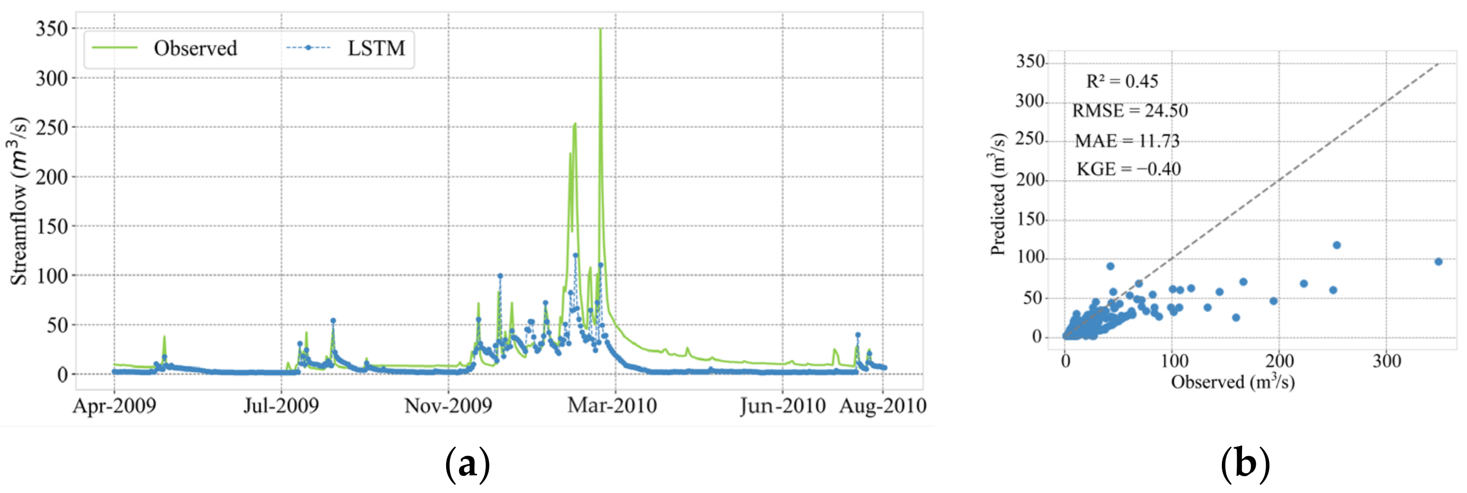
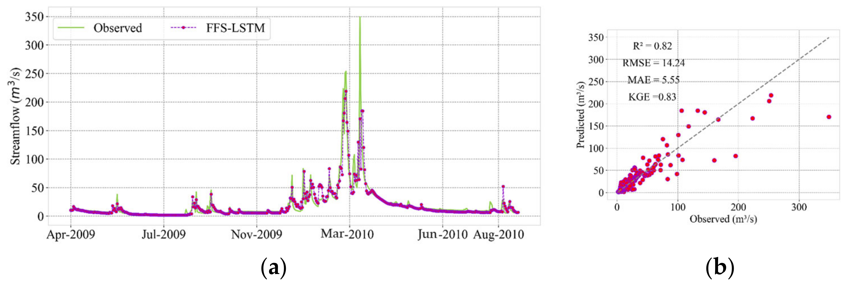
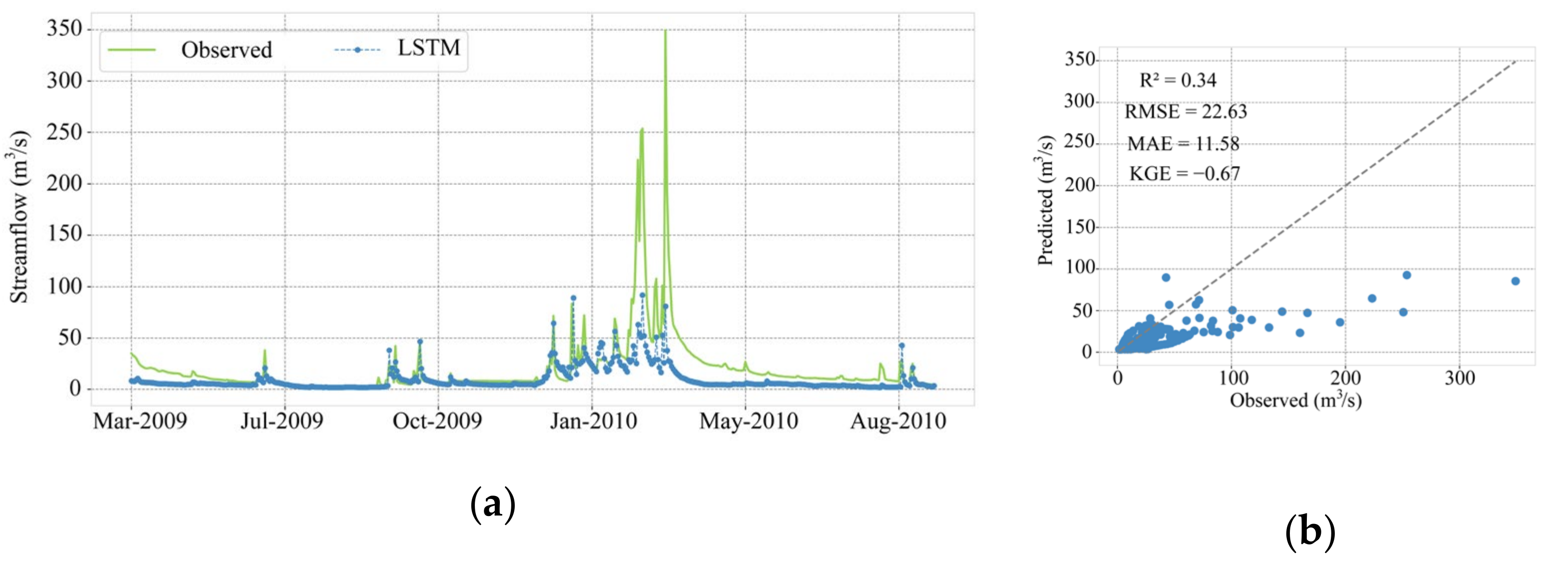
The quantitative analysis of the model behavior (Table 4) using approach 1, illustrates that LSTM (scenario 1) achieved extremely high RMSE and MAE values, shallow values for R2, and negative KGEs. However, the performance of LSTM increases with the number of time steps in predicting results. Thus, the LSTM network hardly remembers the sequence using 2 days of data as input for predicting the next day’s flow. This is mainly due to the memory challenge in watersheds involving the snow and, thus, the lag between the rainfall and streamflow peaks. The results produced under the first input scenario in the validation and testing periods demonstrate that the model is unable to simulate daily streamflow in this study region, where the higher values of R2 were found at TS = 30 (0.75 in training, 0.46 in validation and 0.45 in testing), due to the memory data feature of LSTM that was insufficient to feed the model. In addition, the achievement of the model decreased during testing using approach 2 (Table 5), considering the start and the end of the hydrological year from 1 September 2001 to 31 August 2007 as the training samples, where the best statistical data found at TS = 25 days with R2 = 0.71, 0.51 and 0.34 after training, validation, and testing, respectively. This is mainly due to the meteorological input data and the strong spatiotemporal variability of rainfall. When defining an LSTM network, the network assumes more samples and requires the number of time steps and features to be specified. A time step presents one point of observation in a sample, and a feature is one observation at a time step. Thus, adding lagged data during training could lead LSTM to catch how water is lagged and moved into the watershed, which is interesting for improving model performance. This notion is demonstrated in the second scenario (FFS-LSTM). The values of RMSE, MAE, KGE, and R2 in learning, validation, and predicting sets indicated upstanding streamflow simulation capacity of the LSTM model at TS10 (approach 1) and TS20 (approach 2). Thus, there is a change in KGE, and R2 distribution values of LSTM between different periods at TS2, TS25, and TS30. This finding indicates that the generalization of the LSTM model may considerably compromise the appearance of an extreme event, where the LSTM memory cell holds the previous streamflow values to predict the current streamflow. However, in the first approach, when the sequence length was 25 days the model tended to overfit in the testing phase, with a significant decrease in KGE. For both scenarios, the RMSE and MAE decrease with the time step. These results show that the model has the capability to catch the long-term streamflow components, as well as the reliability of LSTM using the second scenario with both approaches.
Figure 6, Figure 7, Figure 8 and Figure 9 shows the best hydrographs and scatterplots of the observed versus predicted daily streamflow during the testing phase. The green line represents the observed daily streamflow, and the blue and the purple lines represent the prediction results from LSTM and FFS-LSTM scenarios, respectively. Moreover, the time series plots in Figure 6 and Figure 7 show the testing results of the first approach, while Figure 8 and Figure 9 show the same results adopting the second approach. From the figures, it appears that the results from both scenarios using the first approach (70% of training data) had a significantly similar hydrographic form as the second approach (considering the hydrological year). This is mainly due to the period of the training and validation datasets that were almost identical.
The performance of the model using the first input scenario LSTM almost simulates the low flow data. However, at some points it underestimated the flow occurrence which is vital for water supply planning and the preservation of a quantity of water for irrigation. Moreover, as the extreme peak volumes are essential to monitoring flood and disaster events, the second input scenario almost captured the peak flow events using approach 1 with a flow volume of 223 m3/s (Figure 7). The maximum volume caught using approach 2 was 241 m3/s (Figure 9). In the scatterplots (Figure 6b and Figure 8b), the points between the simulated and observed streamflow show that the model has underestimated the actual streamflow, since most of the points were under the diagonal line 1:1; this should be attributed to the size of the time-series data. The randomly split approaches have improved their capacity to predict streamflow using the LSTM model with the second scenario, and fail using the first scenario. However, with FFS-LSTM, it is important to evaluate the training data period, since the model performance may depend on the input data. Therefore, we used an automatic splitting approach named cross-validation to evaluate the model performance in different training times.

3.2. Evaluation of Model Performance with Automatically Split

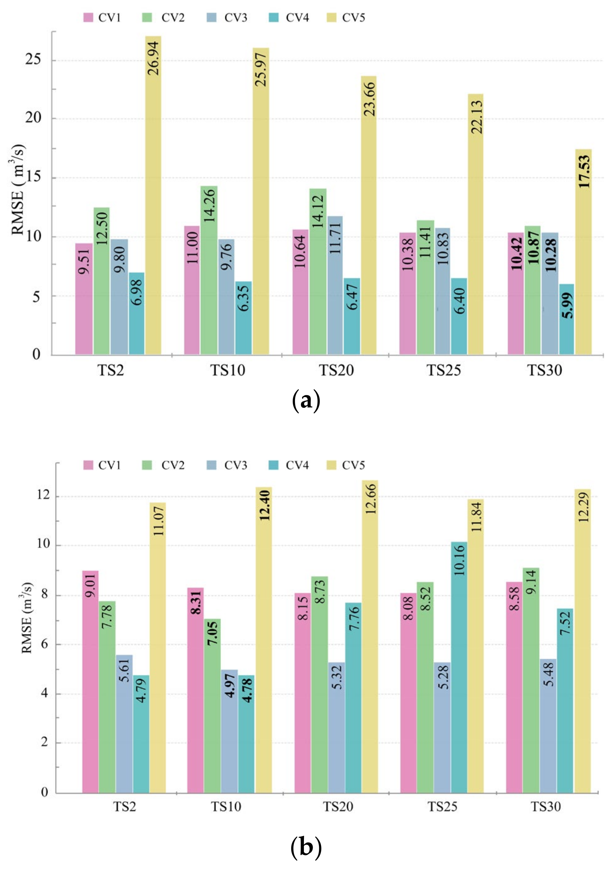
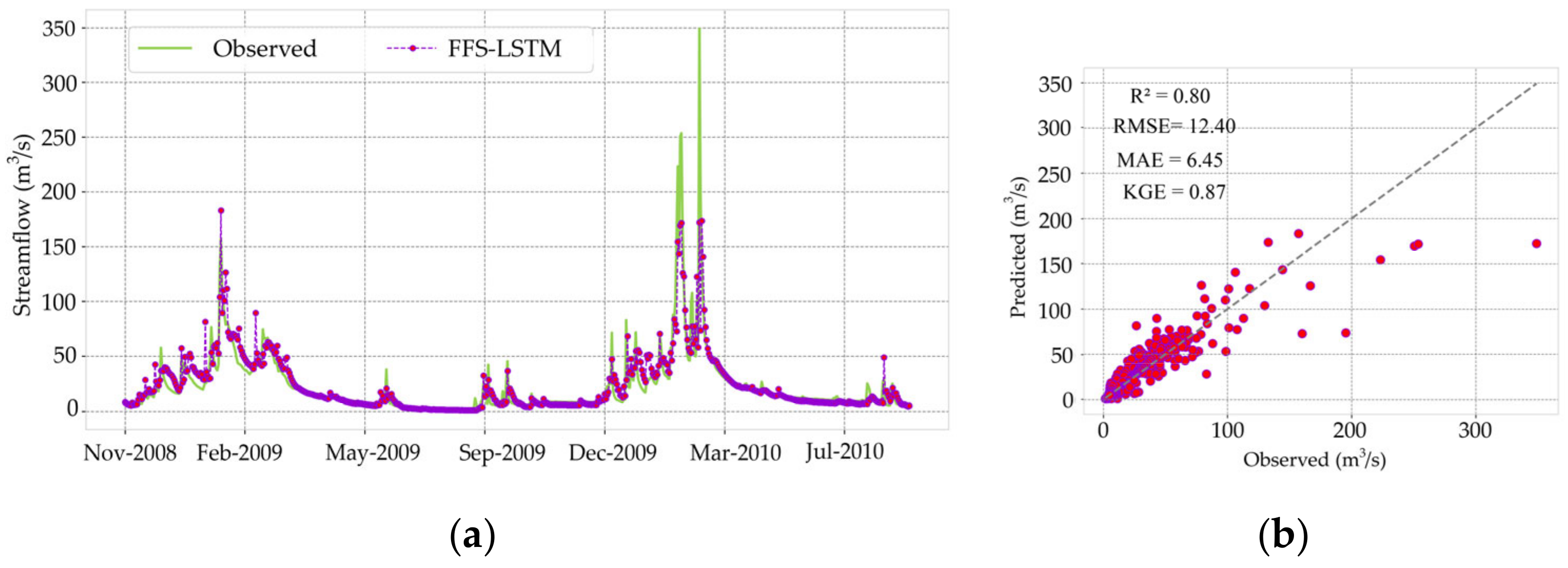
The results of the third approach are summarized in Table 6 and Table 7. Only the scores of sequence lengths TS30 for scenario 1 and TS10 for scenario 2 are shown, comparing the splitting training period on the performance of the model. The outcomes using FFS-LSTM appear to be much more effective than those of LSTM (scenario 1). It produced higher R2, NSE, and KGE in iterations 2 and 5. Lower scores set in CV = 1 due to the learning data that was taken from the end of the series. Decreasing time steps with fewer features impairs the ability to carry informative signals through time, which makes the prediction for the test data less efficient and probably makes the prediction erroneous. The performance at 10 and 30 days in approach 3 with both scenarios increases with the number of iterations, due to the splitting of the learning period that has an influence on the memory of the LSTM network. The bold values of RMSE (Table 6) were compared with the results performance of different time steps (Figure 10a). As may be seen in Figure 10a, the values of RMSE decrease with the number of time steps at CV5, which shows the superiority of the long-term storage memory (LSTM) unit state. However, the performance values of FFS-LSTM (Figure 10b) were quite stable and not affected by the splitting time zone of the data. In addition, at TS = 25 the testing period from 25 January 2007–11 November 2008 has a high RMSE with 10.16 m3/s, due to the chronological data splitting that was a discrepancy at this time step. With the results performance using scenario 1, without adding lagged data as input, the model tends to overfit, thus at CV5 it was reliable. In addition, when using the lagged data, there is a variation of KGE values during the training, validation and testing at the first four folds. Thus, the high values of RMSE in the CV5 are due to the period of training the dataset and the testing data, where the five-fold of the cross-validation was tested with a year that has a high flow volume over 349 m3/s (Figure 2). During the testing phase at TS10 using FFS-LSTM at CV1, CV2, CV3, CV4 and CV5, the values of RMSE are 8.31 m3/s, 7.05 m3/s, 4.97 m3/s, 4.78 m3/s and 12.40 m3/s, respectively, with the maximum observed streamflow of 232.88 m3/s, 294.78 m3/s, 72.86 m3/s, 75.90 m3/s and 349.06 m3/s, respectively. The flow volume variation influences the changes in the RMSE outputs. Similar to the first scenario, the high RMSE is related to the flow regime.
For better visualization of the model’s performance, only the best hydrograph using the FFS-LSTM scenario at iteration 5 is shown in Figure 11. Compared to the previous approaches, the values of the prediction are almost the same due to the size of the learning set, which is nearly identical to approach 1 and approach 2. However, the outputs values of FFS-LSTM in approach 2 are slightly higher than that of approaches 1 and 3 in terms of peak streamflow values. Clearly, the model is not highly affected by the condition of the hydrological year in splitting as well as the splitting time. The prediction results of the FFS-LSTM model with the third approach overestimated the daily streamflow in the periods January 2009 and August 2010. Previous studies have reported the importance of the input sequences length on the storage capability of the basin, and the sensitivity of this hyperparameter over the overfitting predictions issues [30,33]. In our study, the analysis of the sequence length over the three approaches has been improved to capture the dynamics of the daily streamflow prediction.

3.3. Reliability of LSTM Model

The upstanding results yielded by the FFS-LSTM scenario may be explained by the structure of LSTM, which has an intelligent architecture based on memory cells that retained valuable information over a longer period of time by serval memory cells that could filter and keep the data. The LSTM model’s capacity to almost capture the peak of 241 m3/s was carried out into the prediction period. This is a powerful set that the LSTM model provides, with relatively high precision for streamflow in small volumes. Moreover, in our study, we also focused on the impact of the splitting time zone. The performance of the model has compared the random splitting over two approaches, using the end and the start of the hydrological year during the splitting that describes a time period of 12 months, and the chronological time splitting that was defined by the cross-validation using two scenarios. According to the results, almost all the low values were apprehended by the model using the three approaches. The overestimation of the model in the testing set was found mostly in the third approach (Figure 11), on account of the reliability of the LSTM model to the hydrological variables leading inputs (the learning data). Moreover, the achievement of the LSTM model in simulating streamflow using short-term datasets with the first scenario is less improved compared to the conceptual hydrological model’s results, due to the data requirement by deep learning [9]. In most of the studies that used the LSTM model as a setting in hydrological problems, the 3D inputs weren’t a priority. In our study, we used the FFS method as a key solution to determine the optimal input combinations utilizing the optimum time step. Hence, in the process of developing the model, the historical input features play an essential role in the model achievement as well as the length of time steps. The results performed by FFS demonstrate the capability to choose the appropriate predictors when adjusting the sequence length, to avoid the issue of overfitting. In addition, the main problem that causes the overfitting is the data scarcity, with all the models tested used on a limited time series dataset. Hence, the LSTM model may not be sufficiently informed with the watershed hydrological processes that may have a difference between streamflow and rainfall. This discrepancy was described by Ávila et al. using hydrological models [56]. It is worth highlighting that the LSTM model is capable of achieving good predictability performance with all approaches at TS10 and TS20. Based on these results, the selection of the appropriate 3D input combinations and time lag supports the LSTM model to be more reliable. The past histories of each variable with the time steps used in the model can affect streamflow prediction. It enables the model to capture the heading of the time-series dataset, demonstrates a powerful capacity of prediction, and empowers the memory process throughout the LSTM model. In this model, the structure used information about previous computations from specific previous steps to determine whether or not this instruction should be passed on to the next iteration. Since the LSTM model generates the data in numerous time steps, the input data are utilized to update a set of parameters in the internal memory cell states at each step during a training period. Memory cell states are only influenced throughout the prediction period by the input at a single time step and the states from the previous time step. However, machine learning methods such as the ANN model lack a chronological recall and presume that the model’s inputs are independent of one another, making it impossible to detect temporal changes. As a result, the model’s memory cells help the LSTM model better capture dataset trends and demonstrate its predictive power. However, the LSTM was unable to predict streamflow when using the default data as inputs. This demonstrates that the datasets were not enough to feed the model to capture the streamflow.

4. Conclusions

Accurate streamflow prediction has always been one of the primary concerns in watershed management. In this work, we studied the flexibility of the data-driven LSTM model on the streamflow prediction over a semi-arid region. Comprehensively, the LSTM model was tested based on three input conditions. It has been concluded that, the hydrological year (approach 2) and the time splitting zone (approach 3) does not significantly affect the performance of the model, where the accurate time step number is related to the selection of input feature. On the other hand the model shows upstanding performance in recording the streamflow time series using the Forward Feature Selection technique, compared with the default data as input features where the model shows a bad reaction. The FFS method of streamflow decomposition is a meticulous process that significantly improved prediction accuracy using the LSTM model.
The outcomes of the analyses used in this study, illustrate the major issues connected with hydrological modeling studies, particularly the high connection between the LSTM design and the significant impact of input condition circumstances. However, in some of our findings, the model showed overfitting prediction issues due to the scarcity of useful information on ground data, which present the limitations of our study.
In conclusion, the streamflow experiments carried out by LSTM model, learning from meteorological data and satellite data of the studied watershed were impressive. Yet, it is necessary to investigate the stability of the LSTM model, which would be our priority in future studies.

Author Contributions

Study conceptualization, K.N. and A.B.; Data processing and modeling tasks, K.N. and H.O.; analysis, and result interpretation, K.N. and A.B.; writing—original draft preparation, K.N.; writing—review and editing, A.B., H.E., B.B., H.O. and A.C. All authors have read and agreed to the published version of the manuscript.

Funding

This research received no external funding.

Data Availability Statement

The data are not publicly available, authors don’t have permission to share data acquired by hydraulic agency.

Acknowledgments

A.B. (Abdelghani Boudhar) and A.C. are supported by the research program “MorSnow-1”, International Water Research Institute (IWRI), Mohammed VI Polytechnic University (UM6P), Morocco, (Accord spécifique n° 39 entre OCP S.A et UM6P). We thank the Oum Er-Rbia Hydraulic Basin Agency for providing the observed data used in this study. We thank the anonymous reviewers for their helpful and constructive reviews.

Conflicts of Interest

The authors declare no conflict of interest.

References

  1. Fniguire, F.; Laftouhi, N.; Saidi, M.; Zamrane, Z.; El Himer, H.; Khalil, N. Spatial and temporal analysis of the drought vulnerability and risks over eight decades in a semi-arid region (Tensift basin: Morocco). Theor. Appl. Climatol. 2017, 130, 321–330. [Google Scholar] [CrossRef]
  2. Zkhiri, W.; Tramblay, Y.; Hanich, L.; Jarlan, L.; Ruelland, D. Spatiotemporal characterization of current and future droughts in the High Atlas basins (Morocco). Theor. Appl. Climatol. 2019, 135, 593–605. [Google Scholar] [CrossRef]
  3. Ouatiki, H.; Boudhar, A.; Tramblay, Y.; Jarlan, L.; Benabdelouhab, T.; Hanich, L.; El Meslouhi, M.R.; Chehbouni, A. Evaluation of TRMM 3B42 V7 rainfall product over the Oum Er Rbia watershed in Morocco. Climate 2017, 5, 1. [Google Scholar] [CrossRef]
  4. Jarlan, L.; Khabba, S.; Er-Raki, S.; Le Page, M.; Hanich, L.; Fakir, Y.; Merlin, O.; Mangiarotti, S.; Gascoin, S.; Ezzahar, J.; et al. Remote Sensing of Water Resources in Semi-Arid Mediterranean Areas: The joint international laboratory TREMA. Int. J. Remote Sens. 2015, 36, 4879–4917. [Google Scholar] [CrossRef]
  5. Apaydin, H.; Sattari, M.T.; Falsafian, K.; Prasad, R. Artificial intelligence modelling integrated with Singular Spectral analysis and Seasonal-Trend decomposition using Loess approaches for streamflow predictions. J. Hydrol. 2021, 600, 126506. [Google Scholar] [CrossRef]
  6. Boudhar, A.; Ouatiki, H.; Bouamri, H.; Lebrini, Y.; Karaoui, I.; Hssaisoune, M.; Arioua, A.; Benabdelouahab, T. Hydrological Response to Snow Cover Changes Using Remote Sensing over the Oum Er Rbia Upstream Basin, Morocco; Springer International Publishing: Berlin/Heidelberg, Germany, 2020. [Google Scholar]
  7. Besaw, L.; Rizzo, D.; Bierman, P.; Hackett, W. Advances in ungauged streamflow prediction using artificial neural networks. J. Hydrol. 2010, 386, 27–37. [Google Scholar] [CrossRef]
  8. Devi, G.; Ganasri, B.; Dwarakish, G. A Review on Hydrological Models. Aquat. Procedia 2015, 4, 1001–1007. [Google Scholar] [CrossRef]
  9. Ouatiki, H.; Boudhar, A.; Ouhinou, A.; Beljadid, A.; Leblanc, M.; Chehbouni, A. Sensitivity and interdependency analysis of the HBV conceptual model parameters in a semi-arid mountainous watershed. Water 2020, 12, 2440. [Google Scholar] [CrossRef]
  10. Hu, C.; Wu, Q.; Li, H.; Jian, S.; Li, N.; Lou, Z. Deep learning with a long short-term memory networks approach for rainfall-runoff simulation. Water 2018, 10, 1543. [Google Scholar] [CrossRef] [Green Version]
  11. Yang, S.; Yang, D.; Chen, J.; Santisirisomboon, J.; Lu, W.; Zhao, B. A physical process and machine learning combined hydrological model for daily streamflow simulations of large watersheds with limited observation data. J. Hydrol. 2020, 590, 125206. [Google Scholar] [CrossRef]
  12. Botsis, D.; Latinopoulos, P.; Diamantaras, K. Rainfall–Runoff Modeling Using Support Vector Regression and Artificial Neural Networks. Cest2011 2011, No. January. Available online: http://aetos.it.teithe.gr/~kdiamant/docs/CEST2011.pdf (accessed on 2 November 2022).
  13. Chanklan, R.; Kaoungku, N.; Suksut, K.; Kerdprasop, K.; Kerdprasop, N. Runoff prediction with a combined artificial neural network and support vector regression. Int. J. Mach. Learn. Comput. 2018, 8, 39–43. [Google Scholar] [CrossRef] [Green Version]
  14. Hadi, S.; Tombul, M. Forecasting Daily Streamflow for Basins with Different Physical Characteristics through Data-Driven Methods. Water Resour. Manag. 2018, 32, 3405–3422. [Google Scholar] [CrossRef]
  15. Parisouj, P.; Mohebzadeh, H.; Lee, T. Employing Machine Learning Algorithms for Streamflow Prediction: A Case Study of Four River Basins with Different Climatic Zones in the United States. Water Resour. Manag. 2020, 34, 4113–4131. [Google Scholar] [CrossRef]
  16. Ha, S.; Liu, D.; Mu, L. Prediction of Yangtze River streamflow based on deep learning neural network with El Niño–Southern Oscillation. Sci. Rep. 2021, 11, 1–23. [Google Scholar] [CrossRef]
  17. Lai, G. Modeling Long- and Short-Term Temporal Patterns with Deep Neural Networks. In Proceedings of the 41st International ACM SIGIR Conference on Research & Development in Information Retrieval, Ann Arbor, MI, USA, 8–12 July 2018; pp. 95–104. [Google Scholar]
  18. Hu, J.; Wang, X.; Zhang, Y.; Zhang, D.; Zhang, M.; Xue, J. Time Series Prediction Method Based on Variant LSTM Recurrent Neural Network. Neural Process. Lett. 2020, 52, 1485–1500. [Google Scholar] [CrossRef]
  19. Hochreiter, S.; Schmidhuber, J. Long Short-Term Memory. Neural Comput. 1997, 9, 1735–1780. [Google Scholar] [CrossRef]
  20. Kratzert, F.; Klotz, D.; Brenner, C.; Schulz, K.; Herrnegger, M. Rainfall-Runoff modelling using Long-Short-Term-Memory (LSTM) networks. Hydrol. Earth Syst. Sci. Discuss. 2018, 22, 1–26. [Google Scholar] [CrossRef] [Green Version]
  21. Boulmaiz, T.; Guermoui, M.; Boutaghane, H. Impact of training data size on the LSTM performances for rainfall–runoff modeling. Model. Earth Syst. Environ. 2020, 6, 2153–2164. [Google Scholar] [CrossRef]
  22. Kao, I.; Zhou, Y.; Chang, L.; Chang, F. Exploring a Long Short-Term Memory based Encoder-Decoder framework for multi-step-ahead flood forecasting. J. Hydrol. 2020, 583, 124631. [Google Scholar] [CrossRef]
  23. Apaydin, H.; Feizi, H.; Sattari, M.; Colak, M.; Shamshirband, S.; Chau, K. Comparative analysis of recurrent neural network architectures for reservoir inflow forecasting. Water 2020, 12, 1500. [Google Scholar] [CrossRef]
  24. Cheng, M.; Fang, F.; Kinouchi, T.; Navon, I.; Pain, C. Long lead-time daily and monthly streamflow forecasting using machine learning methods. J. Hydrol. 2020, 590, 125376. [Google Scholar] [CrossRef]
  25. Mao, G.; Wang, M.; Liu, J.; Wang, Z.; Wang, K.; Meng, Y.; Zhong, R.; Wang, H.; Li, Y. Comprehensive comparison of artificial neural networks and long short-term memory networks for rainfall-runoff simulation. Phys. Chem. Earth 2021, 123, 103026. [Google Scholar] [CrossRef]
  26. Ouma, Y.; Cheruyot, R.; Wachera, A. Rainfall and runoff time-series trend analysis using LSTM recurrent neural network and wavelet neural network with satellite-based meteorological data: Case study of Nzoia hydrologic basin. Complex Intell. Syst. 2021, 8, 213–236. [Google Scholar] [CrossRef]
  27. Li, W.; Kiaghadi, A.; Dawson, C. High temporal resolution rainfall–runoff modeling using long-short-term-memory (LSTM) networks. Neural Comput. Appl. 2020, 33, 1261–1278. [Google Scholar] [CrossRef]
  28. Prediction, S. Learning Enhancement Method of Long Short-Term Memory Network and Its Applicability in Hydrological Time Series Prediction. Water 2022, 14, 2910. [Google Scholar]
  29. Kratzert, F.; Klotz, D.; Herrnegger, M.; Sampson, A.; Hochreiter, S.; Nearing, G. Toward Improved Predictions in Ungauged Basins: Exploiting the Power of Machine Learning. Water Resour. Res. 2019, 55, 11344–11354. [Google Scholar] [CrossRef] [Green Version]
  30. Choi, J.; Lee, J.; Kim, S. Utilization of the Long Short-Term Memory network for predicting streamflow in ungauged basins in Korea. Ecol. Eng. 2022, 182, 106699. [Google Scholar] [CrossRef]
  31. Hunt, K.; Matthews, G.; Pappenberger, F.; Prudhomme, C. Using a long short-term memory (LSTM) neural network to boost river streamflow forecasts over the western United States. Hydrol. Earth Syst. Sci. Discuss. 2022, 26, 5449–5472. [Google Scholar] [CrossRef]
  32. Rahimzad, M.; Nia, A.M.; Zolfonoon, H.; Soltani, J.; Mehr, A.D.; Kwon, H. Performance Comparison of an LSTM-based Deep Learning Model versus Conventional Machine Learning Algorithms for Streamflow Forecasting. Water Resour. Manag. 2021, 35, 4167–4187. [Google Scholar] [CrossRef]
  33. Park, K.; Jung, Y.; Kim, K. Determination of Deep Learning Model and Optimum Length of Training Data in the River with Large Fluctuations in Flow Rates. Water 2020, 12, 3537. [Google Scholar] [CrossRef]
  34. El Bilali, A.; Taleb, A.; Brouziyne, Y. Groundwater quality forecasting using machine learning algorithms for irrigation purposes. Agric. Water Manag. 2021, 245, 106625. [Google Scholar] [CrossRef]
  35. Ouatiki, H.; Boudhar, A.; Ouhinou, A.; Arioua, A.; Hssaisoune, M.; Bouamri, H.; Benabdelouahab, T. Trend analysis of rainfall and drought over the Oum Er-Rbia River Basin in Morocco during 1970–2010. Arab. J. Geosci. 2019, 12, 128. [Google Scholar] [CrossRef]
  36. Ouakhir, H.; El Ghachi, M.; Goumih, M.; Hamid, L. Fluvial Dynamic in Oued El Abid Basin: Monitoring and Quantification at an Upstream River Section in Bin El Ouidane Dam—2016/2017-(Central High Atlas/Morocco). Am. J. Mech. Appl. 2020, 8, 47. [Google Scholar] [CrossRef]
  37. Marchane, A.; Jarlan, L.; Hanich, L.; Boudhar, A.; Gascoin, S.; Tavernier, A.; Filali, N.; Le Page, M.; Hagolle, O.; Berjamy, B. Assessment of daily MODIS snow cover products to monitor snow cover dynamics over the Moroccan Atlas mountain range. Remote Sens. Environ. 2015, 160, 72–86. [Google Scholar] [CrossRef]
  38. Uysal, G.; Şensoy, A.; Şorman, A. Improving daily streamflow forecasts in mountainous Upper Euphrates basin by multi-layer perceptron model with satellite snow products. J. Hydrol. 2016, 543, 630–650. [Google Scholar] [CrossRef]
  39. Thapa, S.; Zhao, Z.; Li, B.; Lu, L.; Fu, D.; Shi, X.; Tang, B.; Qi, H. Snowmelt-driven streamflow prediction using machine learning techniques (LSTM, NARX, GPR, and SVR). Water 2020, 12, 1734. [Google Scholar] [CrossRef]
  40. Boudhar, A.; Hanich, L.; Boulet, G.; Duchemin, B.; Berjamy, B.; Chehbouni, A. Evaluation of the Snowmelt Runoff model in the Moroccan High Atlas Mountains using two snow-cover estimates. Hydrol. Sci. J. 2009, 54, 1094–1113. [Google Scholar] [CrossRef] [Green Version]
  41. Fan, H.; Jiang, M.; Xu, L.; Zhu, H.; Cheng, J.; Jiang, J. Comparison of long short term memory networks and the hydrological model in runoff simulation. Water 2020, 12, 175. [Google Scholar] [CrossRef] [Green Version]
  42. Lee, D.; Lee, G.; Kim, S.; Jung, S. Future runoff analysis in the mekong river basin under a climate change scenario using deep learning. Water 2020, 12, 1556. [Google Scholar] [CrossRef]
  43. Kim, T.; Yang, T.; Gao, S.; Zhang, L.; Ding, Z.; Wen, X.; Gourley, J.J.; Hong, Y. Can artificial intelligence and data-driven machine learning models match or even replace process-driven hydrologic models for streamflow simulation? A case study of four watersheds with different hydro-climatic regions across the CONUS. J. Hydrol. 2021, 598, 126423. [Google Scholar] [CrossRef]
  44. Reis, G.B.; Da Silva, D.D.; Fernandes Filho, E.I.; Moreira, M.C.; Veloso, G.V.; De Souza Fraga, M.; Pinheiro, S.A.R. Effect of environmental covariable selection in the hydrological modeling using machine learning models to predict daily streamflow. J. Environ. Manag. 2021, 290, 112625. [Google Scholar] [CrossRef] [PubMed]
  45. Ren, K.; Fang, W.; Qu, J.; Zhang, X.; Shi, X. Comparison of eight fi lter-based feature selection methods for monthly stream fl ow forecasting—Three case studies on CAMELS data sets. J. Hydrol. 2020, 586, 124897. [Google Scholar] [CrossRef]
  46. Singh, D.; Singh, B. Investigating the impact of data normalization on classification performance. Appl. Soft Comput. 2020, 97, 105524. [Google Scholar] [CrossRef]
  47. Bai, P.; Liu, X.; Xie, J. Simulating runoff under changing climatic conditions: A comparison of the long short-term memory network with two conceptual hydrologic models. J. Hydrol. 2021, 592, 125779. [Google Scholar] [CrossRef]
  48. Ahmed, S.; Rahman, S.; San, O.; Rasheed, A.; Navon, I. Memory embedded non-intrusive reduced order modeling of non-ergodic flows. Phys. Fluids 2019, 31, 126602. [Google Scholar] [CrossRef] [Green Version]
  49. Almalaq, A.; Zhang, J. Evolutionary Deep Learning-Based Energy Consumption Prediction for Buildings. IEEE Access 2019, 7, 1520–1531. [Google Scholar] [CrossRef]
  50. Liu, C.; Gu, J.; Yang, M. A Simplified LSTM Neural Networks for One Day-Ahead Solar Power Forecasting. IEEE Access 2021, 9, 17174–17195. [Google Scholar] [CrossRef]
  51. Fu, M.; Fan, T.; Ding, Z.; Salih, S.; Al-Ansari, N.; Yaseen, Z. Deep Learning Data-Intelligence Model Based on Adjusted Forecasting Window Scale: Application in Daily Streamflow Simulation. IEEE Access 2020, 8, 32632–32651. [Google Scholar] [CrossRef]
  52. Hu, Y.; Yan, L.; Hang, T.; Feng, J. Stream-flow forecasting of small rivers based on LSTM. arXiv 2020, arXiv:2001.05681. [Google Scholar]
  53. Zhang, D.; Liu, X.; Bai, P.; Li, X. Suitability of satellite-based precipitation products for water balance simulations using multiple observations in a humid catchment. Remote Sens. 2019, 11, 151. [Google Scholar] [CrossRef] [Green Version]
  54. Knoben, W.; Freer, J.; Woods, R. Technical note: Inherent benchmark or not? Comparing Nash-Sutcliffe and Kling-Gupta efficiency scores. Hydrol. Earth Syst. Sci. 2019, 23, 4323–4331. [Google Scholar] [CrossRef] [Green Version]
  55. Bouabid, R.; Chafai, A.; Alaoui, E.; Bahri, H. Streamflow response to climate variability in sub-watersheds of the Sebou river basin, Morocco. In Proceedings of the EGU General Assembly 2010, Vienna, Austria, 2–7 May 2010; p. 3237. [Google Scholar]
  56. Ávila, L.; Silveira, R.; Campos, A.; Rogiski, N.; Gonçalves, J.; Scortegagna, A.; Freita, C.; Aver, C.; Fan, F. Comparative Evaluation of Five Hydrological Models in a Large-Scale and Tropical River Basin. Water 2022, 14, 3013. [Google Scholar] [CrossRef]
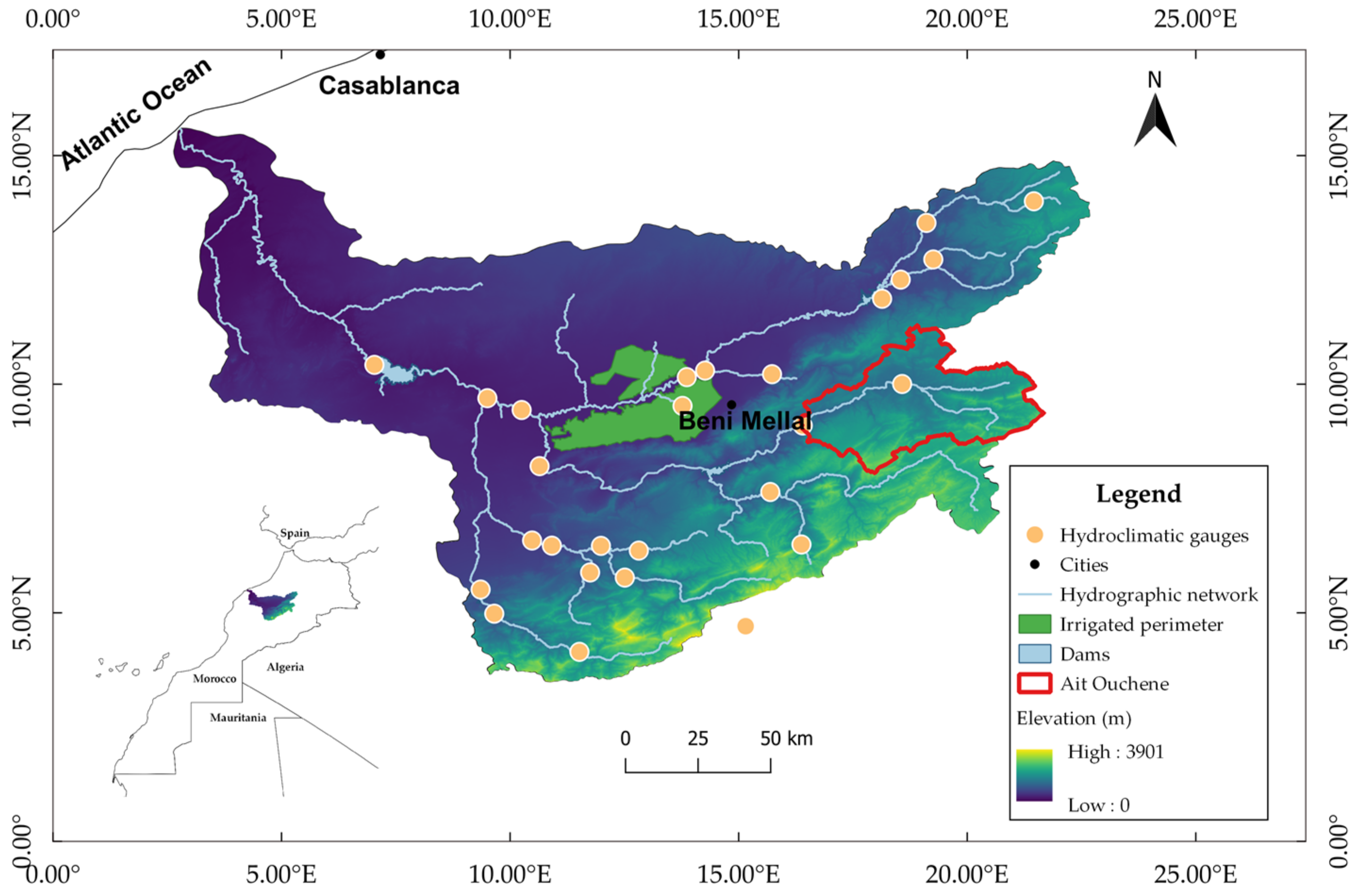
Figure 1. The geographical setting of the study area.
Water 15 00262 g001
Figure 2. Ait Ouchen streamflow and rainfall data used in this study (1 September 2001–31 August 2010).
Water 15 00262 g002
Figure 3. The architecture of Long-Short-Term Memory (LSTM) where σ presents the sigmoid function, tanh the hyperbolic tangent, Ct−1 previous cell state, ht−1 previous hidden state, xt input data, Ct new cell state and ht present the new hidden state. The adding and scaling of information is represented by the vector operations (+) and (X), respectively.
Water 15 00262 g003
Figure 4. Flowchart of the modeling process for streamflow prediction model.
Water 15 00262 g004
Figure 5. Schematic illustration of cross-validation splitting approach.
Water 15 00262 g005
Figure 6. The hydrograph of observed and predicted daily streamflow of LSTM scenario during the testing (a) using approach 1 at TS = 30 along with the corresponding scatter plot (b).
Water 15 00262 g006
Figure 7. The hydrograph of observed and predicted daily streamflow of FFS-LSTM scenario during the testing (a) using approach 1 at TS = 10 along with the corresponding scatter plot (b).
Water 15 00262 g007
Figure 8. The hydrograph of observed and predicted daily streamflow of LSTM scenario during the testing (a) using approach 2 at TS = 25 along with the corresponding scatter plot (b).
Water 15 00262 g008
Figure 9. The hydrograph of observed and predicted daily streamflow of FFS-LSTM scenario during the testing (a) using approach 2 at TS = 20 with the corresponding scatter plot (b).
Water 15 00262 g009
Figure 10. Comparisons of model predictions in different time steps and different data splitting during the testing phase using approach 3 (a) LSTM. (b) FFS-LSTM.
Water 15 00262 g010
Figure 11. The hydrograph of observed and predicted daily streamflow of FFS-LSTM scenario during the testing (a) using approach 3 (CV = 5) at TS = 10 with the corresponding scatter plot (b).
Water 15 00262 g011
Table 1. General characteristics of Ait Ouchen watershed.
WatershedArea (km2)PerimeterAltitude
Min
Altitude
Max
Altitude
Mean
Principal River
Ait Ouchen242732295332301945Oued El Abid
Table 2. Dataset input scenarios.
ScenariosVariables Description
LSTMrainfall (R), temperature (T) and snow cover area (SCA)
FFS-LSTMrainfall, lagged rainfall (1, 2 days), 3 lagged days of streamflow and 2, 3 days lagged SCA
Table 3. Hyper-parameters used for training LSTM network.
Hyper-ParametersSelection
Create LSTMNeurons in the input layer50 neurons
Neurons in the hidden layer20 neurons
Neurons in the output layerOne neuron
Fit LSTMActivation function tanh
Number of Epochs250 epochs
Batch size10, 32
Loss function
Optimizer
Mean Square Error
Adam
Table 4. Performance of the model scenarios for daily streamflow simulation using approach 1 (70% train; 15% valid; 15% test) with a variety of sequence lengths (number of time steps).
ScenariosTrainingValidationTesting
RMSEMAEKGER2RMSEMAEKGER2RMSEMAEKGER2
LSTM
TS2
TS10
TS20
TS25
TS30
9.304.520.300.4318.8610.40−0.650.0731.8614.06−2.770.04
7.443.770.650.6317.699.86−0.810.1929.3213.66−1.880.20
7.493.800.720.6315.389.20−0.120.3927.9813.22−1.240.29
8.855.140.540.4814.189.500.520.4826.2714.07−1.070.35
6.133.230.830.7514.528.570.020.4624.5011.73−0.400.45
FFS-LSTM
TS2
TS10
TS20
TS25
TS30
5.642.280.900.798.854.260.840.8015.085.410.720.78
5.212.150.880.829.274.620.820.7814.245.550.830.82
5.862.540.820.7712.056.200.670.6314.866.350.880.79
4.211.860.930.888.254.050.700.8319.776.760.100.64
5.162.360.900.829.745.720.760.7514.696.070.790.80
Table 5. Performance of the model scenarios for daily streamflow simulation using approach 2 (considering hydrological year) with a variety of sequence lengths (number of time steps).
ScenariosTrainingValidationTesting
RMSEMAEKGER2RMSEMAEKGER2RMSEMAEKGER2
LSTM
TS2
TS10
TS20
TS25
TS30
9.594.160.260.4210.905.820.310.2929.5815.00−2.39−0.04
8.834.550.570.5610.135.820.440.3927.3514.10−1.430.13
8.174.800.540.5810.496.390.300.3524.3912.39−1.090.22
6.814.010.740.719.215.240.580.5122.6311.58−0.670.34
8.474.800.480.5511.326.640.020.2523.9211.87−1.050.25
FFS-LSTM
TS2
TS10
TS20
TS25
TS30
7.092.740.750.687.573.630.750.6613.875.570.760.78
6.332.720.790.758.534.010.720.5714.825.950.860.75
4.832.620.780.857.974.060.760.6311.214.810.810.84
5.522.520.780.817.343.770.780.6911.314.500.750.84
5.802.930.750.789.224.800.660.5110.955.170.840.83
Table 6. Performance of the LSTM scenario for daily streamflow simulation using approach 3 (cross-validation) at TS = 30.
ScenarioTrainingValidationTesting
RMSEMAEKGER2RMSEMAEKGER2RMSEMAEKGER2
LSTM
CV111.45.72−0.390.3726.3212.56−3.030.0610.424.45−0.430.2
CV28.275.270.380.623.5511.56−1.340.2510.875.440.120.55
CV37.144.540.630.7723.2611.33−1.240.2710.286.290.450.01
CV48.915.980.430.6622.6810.8−1.040.35.994.990.40.28
CV58.14.860.620.66.134.130.580.2817.5310.410.540.58
Table 7. Performance of FFS-LSTM scenario for daily streamflow simulation using approach 3 (cross-validation) at TS = 10.
ScenarioTrainingValidationTesting
RMSEMAEKGER2RMSEMAEKGER2RMSEMAEKGER2
FFS-LSTM
CV15.12.120.750.8712.714.950.480.788.312.280.260.51
CV24.982.620.860.8513.34.730.450.767.052.90.70.8
CV35.262.50.870.8714.115.630.30.734.972.240.80.77
CV45.83.480.650.8513.276.80.50.764.783.1−0.010.53
CV56.012.640.80.784.472.040.80.6212.46.450.870.8
Disclaimer/Publisher’s Note: The statements, opinions and data contained in all publications are solely those of the individual author(s) and contributor(s) and not of MDPI and/or the editor(s). MDPI and/or the editor(s) disclaim responsibility for any injury to people or property resulting from any ideas, methods, instructions or products referred to in the content.