
Assessing Flood Risk: LH-Moments Method and Univariate Probability Distributions in Flood Frequency Analysis


Abstract
:1. Introduction and Background
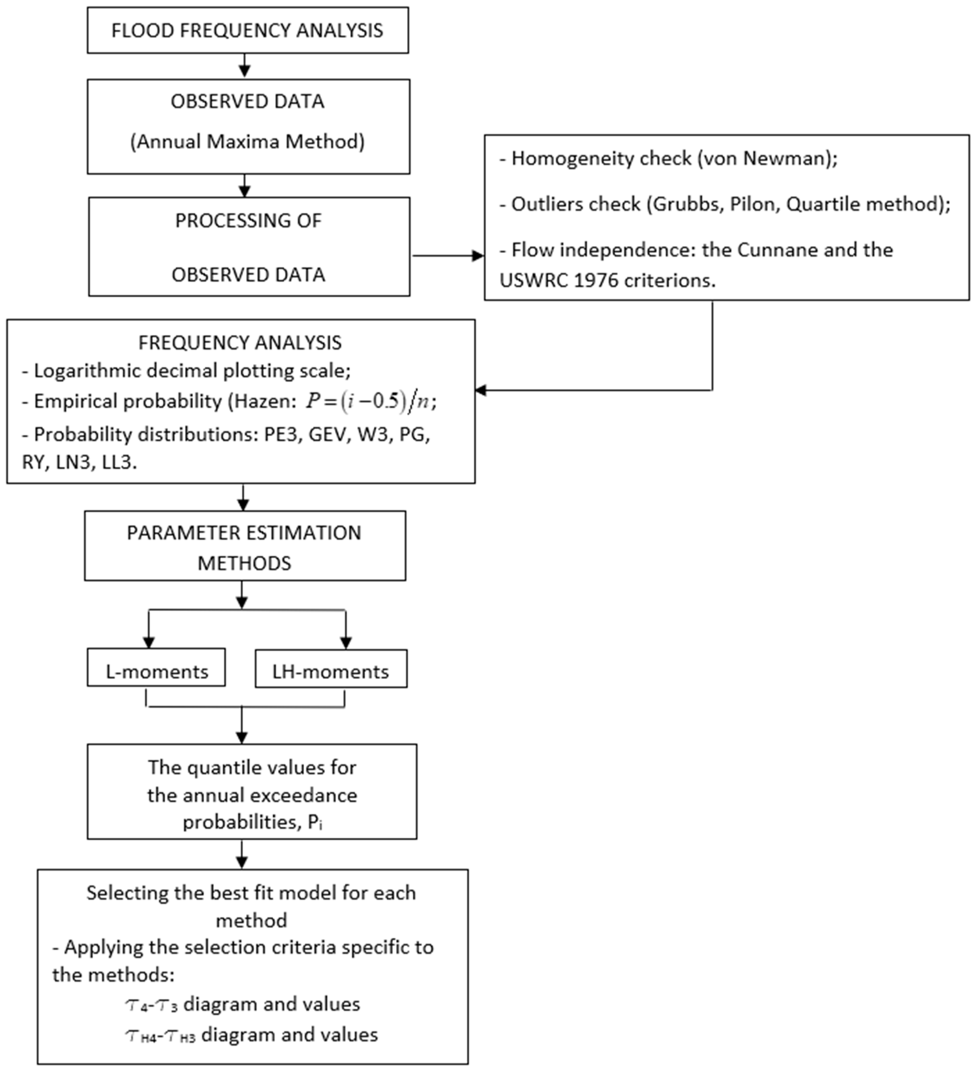
2. Methods
2.1. Probability Distributions
2.2. Parameter Estimation Methods
2.3. The Bias Due to the Length Variability of the Records
2.3.1. The Bias for Statistical Indicators
2.3.2. The Bias of Parameter Estimation
2.3.3. The Bias of Quantiles Estimation
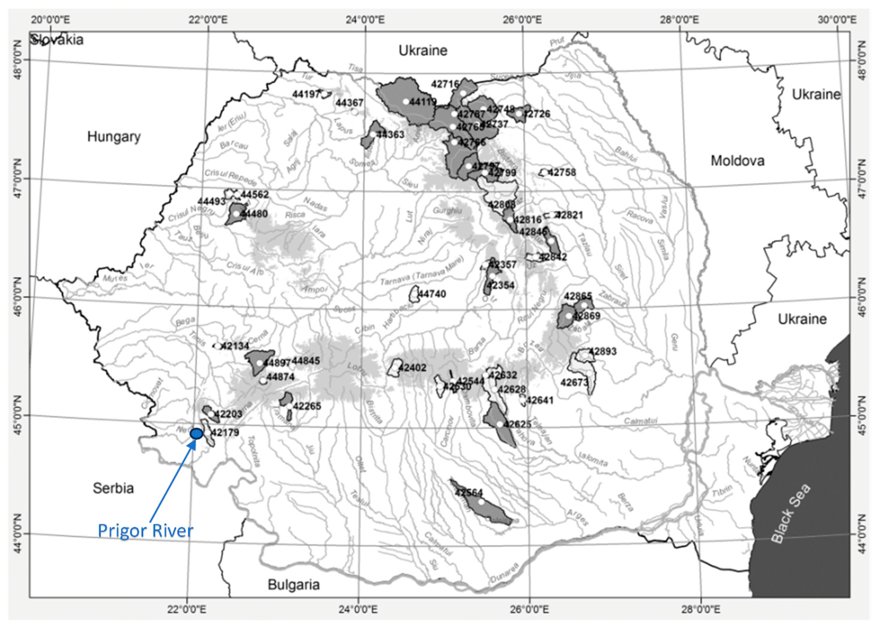
3. Case Study
4. Results and Discussion
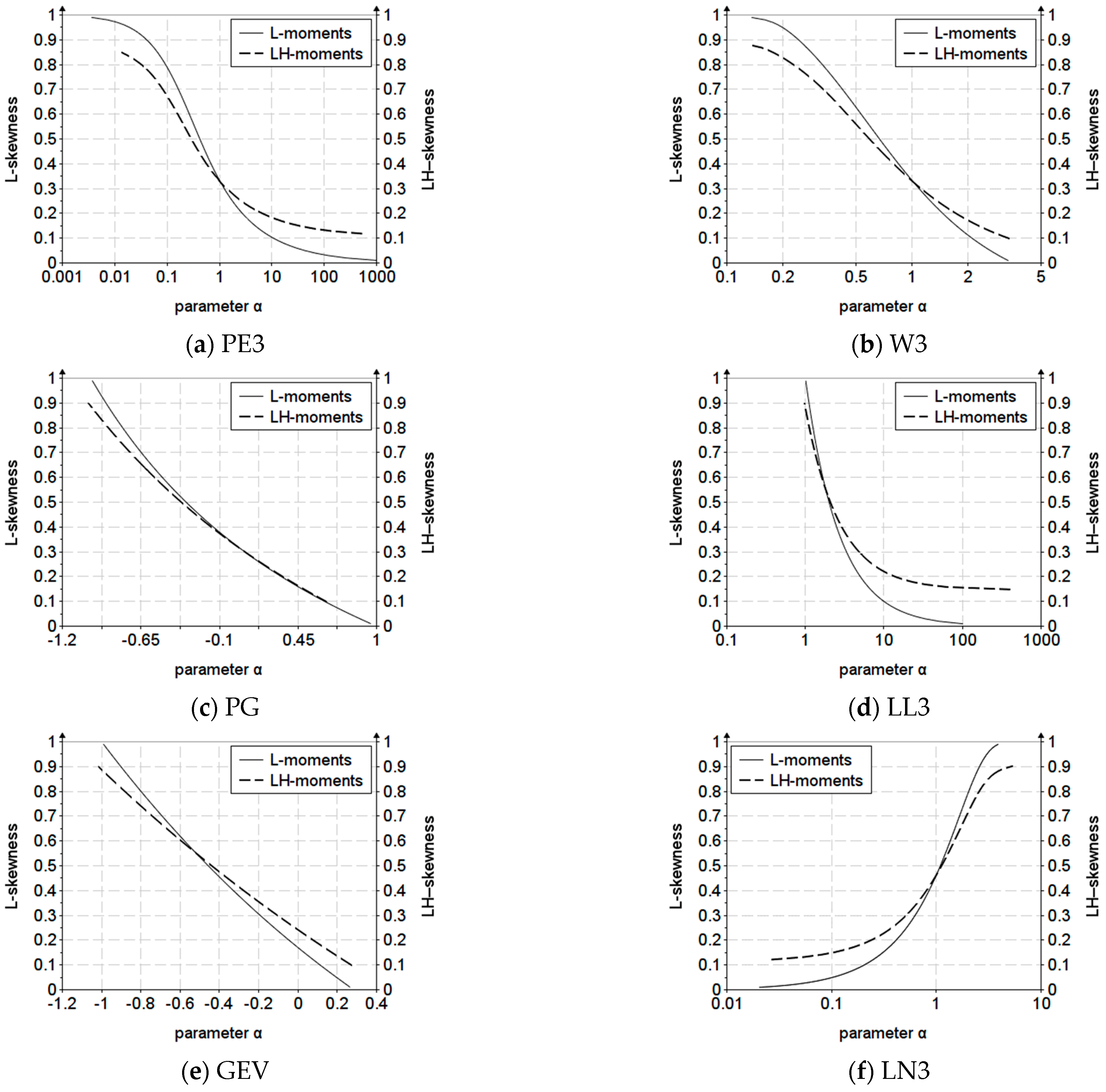
4.1. Parameter Estimation
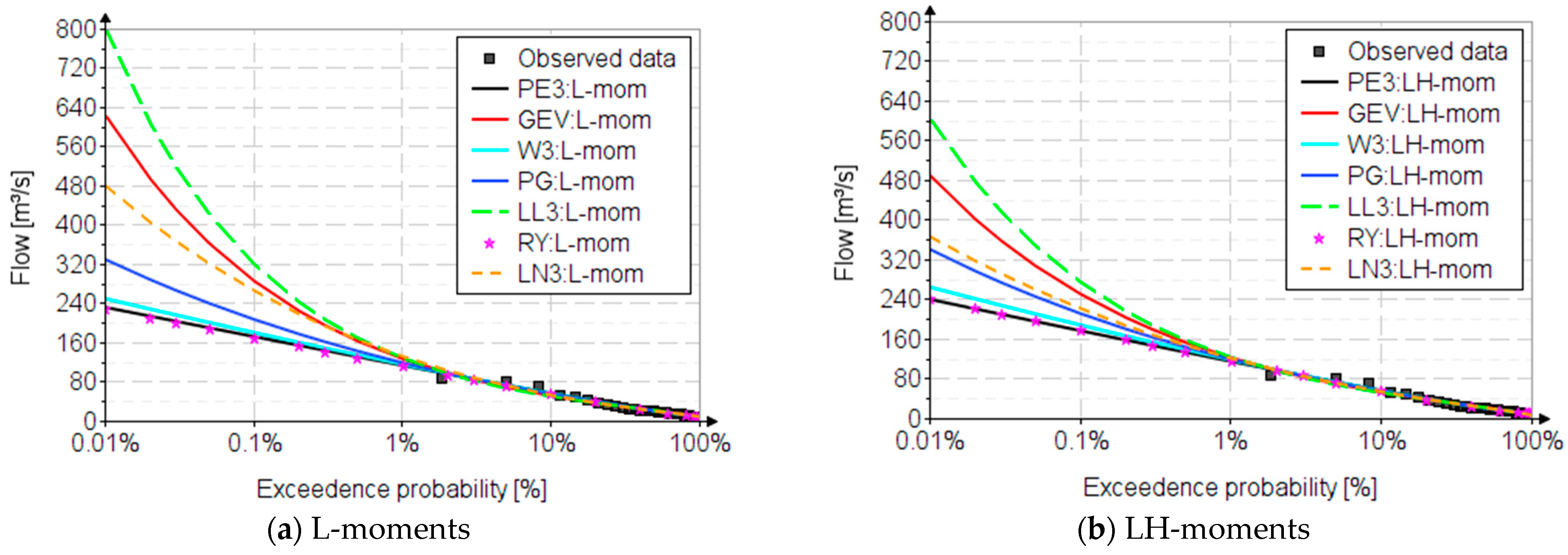
4.2. Quantile Estimation
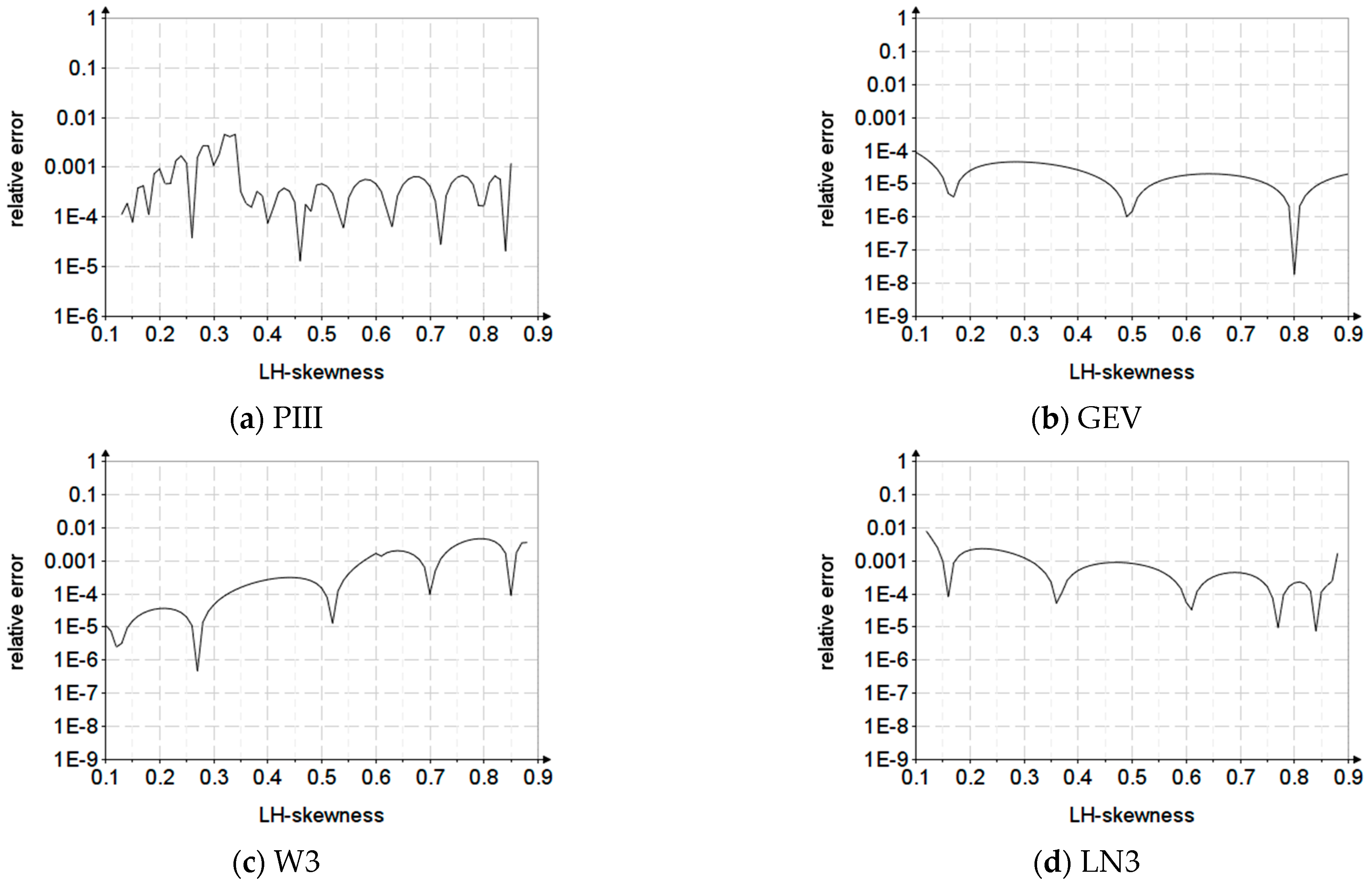
4.3. Performance Metrics
4.4. The Bias Due to the Length Variability of the Records
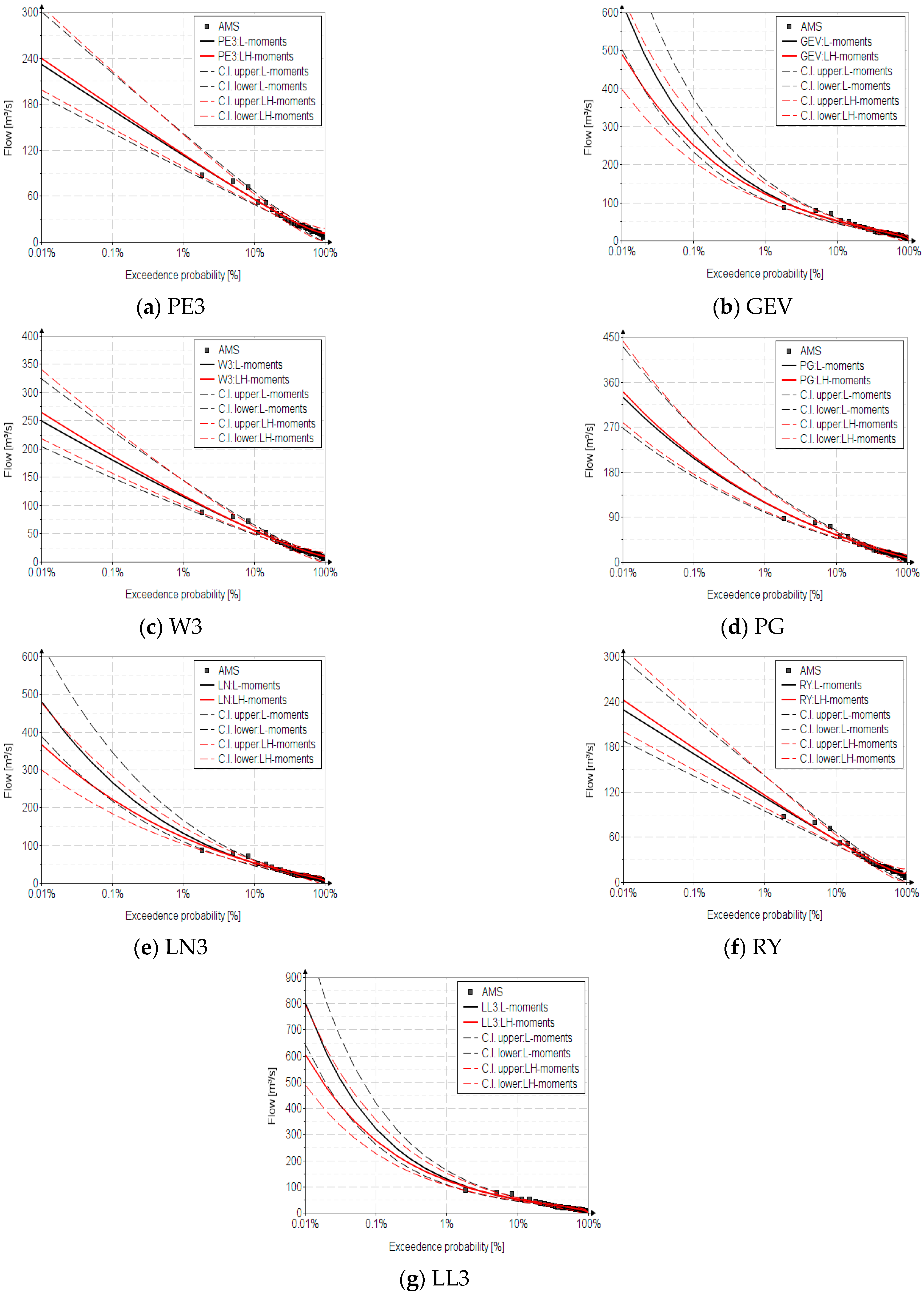
4.5. Confidence Intervals
5. Conclusions
Supplementary Materials
Author Contributions
Funding
Data Availability Statement
Conflicts of Interest
Abbreviations
| MOM | The method of ordinary moments |
| L-moments | The method of linear moments |
| LH-moments | The method of higher order linear moments |
| LH-skewness | |
| coefficient of LH variation | |
| LH-kurtosis | |
| Expected value; arithmetic mean | |
| Standard deviation | |
| Variance | |
| Coefficient of variation | |
| Coefficient of skewness; skewness | |
| Coefficient of kurtosis; kurtosis | |
| Linear moments | |
| Coefficient of variation based on the L-moments method | |
| Coefficient of skewness based on the L-moments method | |
| Coefficient of kurtosis based on the L-moments method | |
| FFA | Flood frequency analysis |
| Distr. | Distributions |
| AMS | Annual maximum series |
| RME | Relative mean error |
| RAE | Relative absolute error |
| n | Observed values length |
| , returns the value of the Euler gamma function of | |
| , returns the value of the incomplete gamma function of x with parameter | |
| Returns the inverse cumulative probability distribution for probability p, for gamma distribution | |
| Returns the cumulative probability distribution for value x, for log-normal distribution | |
| Returns the cumulative probability distribution for value x, for normal distribution | |
| Returns the inverse cumulative probability distribution for probability p, for log-normal distribution | |
| Returns the cumulative probability distribution with mean 0 and variance 1 (normal distribution) | |
| Returns the probability density for value x, for normal distribution | |
| Returns the probability density for value x, for log-normal distribution |
Appendix A. The First Order LH-Moments for PE3, GEV, W3, PG, LL3 and RY Distributions
Appendix A.1. Pearson III (PE3)
- if :
- if :
- if :
- if :
- if :
Appendix A.2. Generalized Extreme Value (GEV)
Appendix A.3. Weibull (W3)
- if :
- if :
Appendix A.4. Generalized Pareto (GP)
Appendix A.5. Rayleigh (RY)
Appendix A.6. Log-Normal (LN3)
- if :
- if :
- if :
- , which can be approximated with:
Appendix A.7. Log-Logistic (LL3)
References
- Popovici, A. Dams for Water Accumulations; Technical Publishing House: Bucharest, Romania, 2002; Volume II. [Google Scholar]
- STAS 4068/1-82; Maximum Water Discharges and Volumes, Determination of maximum Water Discharges and Volumes of Watercourses. The Romanian Standardization Institute: Bucharest, Romania, 1982.
- Ilinca, C.; Anghel, C.G. Flood-Frequency Analysis for Dams in Romania. Water 2022, 14, 2884. [Google Scholar] [CrossRef]
- Teodorescu, I.; Filotti, A.; Chiriac, V.; Ceausescu, V.; Florescu, A. Water Management; Ceres Publishing House: Bucharest, Romania, 1973. [Google Scholar]
- Hosking, J.R.M.; Wallis, J.R. Regional Frequency Analysis: An Approach Based on L–Moments; Cambridge University Press: Cambridge, UK, 1997. [Google Scholar]
- Rao, A.R.; Hamed, K.H. Flood Frequency Analysis; CRC Press LLC.: Boca Raton, FL, USA, 2000. [Google Scholar]
- Singh, V.P. Entropy-Based Parameter Estimation in Hydrology; Springer: Dordrecht, The Netherlands, 1998. [Google Scholar]
- Greenwood, J.A.; Landwehr, J.M.; Matalas, N.C.; Wallis, J.R. Probability Weighted Moments: Definition and Relation to Parameters of Several Distributions Expressible in Inverse Form. Water Resour. Res. 1979, 15, 1049–1054. [Google Scholar] [CrossRef]
- Houghton, C. Birth of a Parent: The Wakeby Distribution for Modeling Flood Flows; Working Paper No. MIT-EL77–033WP; Water Resources Research: Tucson, AZ, USA, 1978; Volume 14. [Google Scholar]
- Hydrology Subcommittee; Interagency Advisory Committee on Water Data; U.S. Department of the Interior; U.S. Geological Survey; Office of Water Data Coordination. Bulletin 17B Guidelines for Determining Flood Flow Frequency; Hydrology Subcommittee; Interagency Advisory Committee on Water Data; U.S. Department of the Interior: Reston, VA, USA; U.S. Geological Survey: Reston, VA, USA; Office of Water Data Coordination: Reston, VA, USA, 1981. [Google Scholar]
- U.S. Department of the Interior; U.S. Geological Survey. Bulletin 17C Guidelines for Determining Flood Flow Frequency; U.S. Department of the Interior: Reston, VA, USA; U.S. Geological Survey: Reston, VA, USA; Office of Water Data Coordination: Reston, VA, USA, 2017. [Google Scholar]
- Ilinca, C.; Anghel, C.G. Frequency Analysis of Extreme Events Using the Univariate Beta Family Probability Distributions. Appl. Sci. 2023, 13, 4640. [Google Scholar] [CrossRef]
- Anghel, C.G.; Ilinca, C. Hydrological Drought Frequency Analysis in Water Management Using Univariate Distributions. Appl. Sci. 2023, 13, 3055. [Google Scholar] [CrossRef]
- Murshed, S.; Park, B.-J.; Jeong, B.-Y.; Park, J.-S. LH-Moments of Some Distributions Useful in Hydrology. Commun. Stat. Appl. Methods 2009, 16, 647–658. [Google Scholar] [CrossRef]
- Hosking, J.R.M. L-moments: Analysis and Estimation of Distributions using Linear, Combinations of Order Statistics. J. R. Statist. Soc. 1990, 52, 105–124. [Google Scholar] [CrossRef]
- Wang, Q.J. LH moments for statistical analysis of extreme events. Water Resour. Res. 1997, 33, 2841–2848. [Google Scholar] [CrossRef]
- Gaume, E. Flood frequency analysis: The Bayesian choice. WIREs Water. 2018, 5, e1290. [Google Scholar] [CrossRef]
- Ilinca, C.; Anghel, C.G. Flood Frequency Analysis Using the Gamma Family Probability Distributions. Water 2023, 15, 1389. [Google Scholar] [CrossRef]
- Hewa, G.A.; Wang, Q.J.; McMahon, T.A.; Nathan, R.J.; Peel, M.C. Generalized extreme value distribution fitted by LH moments for low-flow frequency analysis. Water Resour. Res. 2007, 43, W06301. [Google Scholar] [CrossRef]
- Wang, Q.J. Approximate Goodness-of-Fit Tests of fitted generalized extreme value distributions using LH moments. Water Resour. Res. 1998, 34, 3497–3502. [Google Scholar] [CrossRef]
- Fawad, M.; Cassalho, F.; Ren, J.; Chen, L.; Yan, T. State-of-the-Art Statistical Approaches for Estimating Flood Events. Entropy 2022, 24, 898. [Google Scholar] [CrossRef] [PubMed]
- Lee, S.H.; Maeng, S.J. Comparison and analysis of design floods by the change in the order of LH-moment methods. Irrig. Drain. 2003, 52, 231–245. [Google Scholar] [CrossRef]
- Ali, M.; Khalili, D. Comprehensive evaluation of regional flood frequency analysis by L- and LH-moments. II. Development of LH-moments parameters for the generalized Pareto and generalized logistic distributions. Stoch. Environ. Res. Risk Assess. 2009, 23, 137–152. [Google Scholar]
- Ali, M.; Davar, K. Comprehensive evaluation of regional flood frequency analysis by L- and LH-moments. I. A revisit to regional homogeneity. Stoch. Environ. Res. Risk Assess. 2009, 23, 119–135. [Google Scholar] [CrossRef]
- Abhijit, B.; Munindra, B.; Rakesh, K. Regional Flood Frequency Analysis of North-Bank of the River Brahmaputra by Using LH-Moments. Water Resour. Manag. 2010, 24, 1779–1790. [Google Scholar] [CrossRef]
- Hossein, M.; Gheidari, N. Comparisons of the L- and LH-moments in the selection of the best distribution for regional flood frequency analysis in Lake Urmia Basin. Civ. Eng. Environ. Syst. 2013, 30, 72–84. [Google Scholar] [CrossRef]
- Deka, S.; Borah, M.; Kakaty, S.C. Statistical analysis of annual maximum rainfall in North-East India: An application of LH-moments. Theor. Appl. Climatol. 2011, 104, 111–122. [Google Scholar] [CrossRef]
- Zahrahtul, Z.; Jarah, S.; Mumtazimah, M. Rainfall frequency analysis using LH-moments approach: A case of Kemaman Station, Malaysia. Int. J. Eng. Technol. 2018, 7, 107–110. [Google Scholar] [CrossRef]
- Dhruba, B.; Munindra, B.; Abhijit, B. Regional analysis of maximum rainfall using L-moment and LH-moment: A comparative case study for the northeast India. Mausam. 2017, 68, 451–462. [Google Scholar] [CrossRef]
- Anghel, C.G.; Ilinca, C. Predicting Flood Frequency with the LH-Moments Method: A Case Study of Prigor River, Romania. Water 2023, 15, 2077. [Google Scholar] [CrossRef]
- Diacon, C.; Serban, P. Hydrological Syntheses and Regionalizations; Technical Publishing House: Bucharest, Romania, 1994. [Google Scholar]
- Ioanitoaia, R.H. Ameliorative Hydrology; Agro-Silvica Publishing House: Bucharest, Romania, 1962. [Google Scholar]
- Constantinescu, M.; Golstein, M.; Haram, V.; Solomon, S. Hydrology; Technical Publishing House: Bucharest, Romania, 1956. [Google Scholar]
- Chow, V.T.; Maidment, D.R.; Mays, L.W. Applied Hydrology; McGraw-Hill, Inc.: New York, NY, USA, 1988; ISBN 007-010810-2. [Google Scholar]
- Crooks, G.E. Field Guide to Continuous Probability Distributions; Berkeley Institute for Theoretical Science: Berkeley, CA, USA, 2019. [Google Scholar]
- Gubareva, T.S.; Gartsman, B.I. Estimating Distribution Parameters of Extreme Hydrometeorological Characteristics by L-Moment Method. Water Resour. 2010, 37, 437–445. [Google Scholar] [CrossRef]
- Hosking, J.R.M.; Wallis, J.R. Parameter and Quantile Estimation for the Generalized Pareto Distribution. Technometrics 1987, 29, 339–349. [Google Scholar] [CrossRef]
- Kundu, D.; Raqab, Z. Estimation of R=P[Y<X] for three-parameter generalized Rayleigh distribution. J. Stat. Comput. Simul. 2015, 85, 725–739. [Google Scholar] [CrossRef]
- Anghel, C.G.; Ilinca, C. Parameter Estimation for Some Probability Distributions Used in Hydrology. Appl. Sci. 2022, 12, 12588. [Google Scholar] [CrossRef]
- Bîrsan, M.V. The Variability of the Natural Flow Regime of Rivers in Romania; Ars Docendi Publishing House: Bucharest, Romania, 2017. [Google Scholar]
- Ministry of the Environment. The Romanian Water Classification Atlas, Part I—Morpho-Hydrographic Data on the Surface Hydrographic Network; Ministry of the Environment: Bucharest, Romania, 1992. [Google Scholar]
- Yahaya, A.S.; Nor, N.M.; Jali, N.R.M.; Ramli, N.A.; Ahmad, F.; Ul-Saufie, A.Z. Determination of the Probability Plotting Position for Type I Extreme Value Distribution. J. Appl. Sci. 2012, 12, 1501–1506. [Google Scholar]
- Ministry of Regional Development and Tourism. The Regulations Regarding the Establishment of Maximum Flows and Volumes for the Calculation of Hydrotechnical Retention Constructions; Indicative NP 129–2011; Ministry of Regional Development and Tourism: Bucharest, Romania, 2012. [Google Scholar]
- Flowers-Cano, R.S.; Ortiz-Gómez, R.; León-Jiménez, J.E.; López Rivera, R.; Perera Cruz, L.A. Comparison of Bootstrap Confidence Intervals Using Monte Carlo Simulations. Water 2018, 10, 166. [Google Scholar] [CrossRef]
- Rao, G.S.; Albassam, M.; Aslam, M. Evaluation of Bootstrap Confidence Intervals Using a New Non-Normal Process Capability Index. Symmetry 2019, 11, 484. [Google Scholar] [CrossRef]
- Markiewicz, I.; Bogdanowicz, E.; Kochanek, K. Quantile Mixture and Probability Mixture Models in a Multi-Model Approach to Flood Frequency Analysis. Water 2020, 12, 2851. [Google Scholar] [CrossRef]
- Kochanek, K.; Strupczewski, W.G.; Bogdanowicz, E.; Markiewicz, I. The bias of the maximum likelihood estimates of flood quantiles based solely on the largest historical records. J. Hydrol. 2020, 584, 124740. [Google Scholar] [CrossRef]
- Markiewicz, I.; Bogdanowicz, E.; Kochanek, K. On the Uncertainty and Changeability of the Estimates of Seasonal Maximum Flows. Water 2020, 12, 704. [Google Scholar] [CrossRef]
- Anghel, C.G.; Ilinca, C. Evaluation of Various Generalized Pareto Probability Distributions for Flood Frequency Analysis. Water 2023, 15, 1557. [Google Scholar] [CrossRef]
- Drobot, R.; Draghia, A.F.; Chendes, V.; Sirbu, N.; Dinu, C. Consideratii privind viiturile sintetice pe Dunare. Hidrotehnica 2023, 68, 37–52. (In Romanian) [Google Scholar]


| Novelty | Distribution | |
|---|---|---|
| Method | ||
| L-Moment | LH-Moments | |
| Exact parameter estimation | Raylegh | Pearson III, Weibull, log-normal, generalized Pareto, Raylegh, log-logistic |
| Approximate estimation of parameters | GEV, Weibull, generalized Pareto, log-logistic | Pearson III, GEV, Weibull, log-normal, generalized Pareto, Raylegh, log-logistic |
| Expression of the quantile with the frequency factor (FF) | GEV, Weibull, Raylegh, log-normal | Pearson III, GEV, Weibull, log-normal, generalized Pareto, Raylegh, log-logistic |
| Exact relationships of the FF | GEV, Weibull, Raylegh, log-normal | Pearson III, GEV, Weibull, log-normal, generalized Pareto, Raylegh, log-logistic |
| Approximate estimation of the FF | GEV, Weibull, log-normal | Pearson III, GEV, Weibull, log-normal, generalized Pareto, Raylegh, log-logistic |
| The confidence interval with the Chow approach [34] | GEV, Weibull, generalized Pareto, log-normal, Raylegh, log-logistic | Pearson III, GEV, Weibull, log-normal, generalized Pareto, Raylegh, log-logistic |
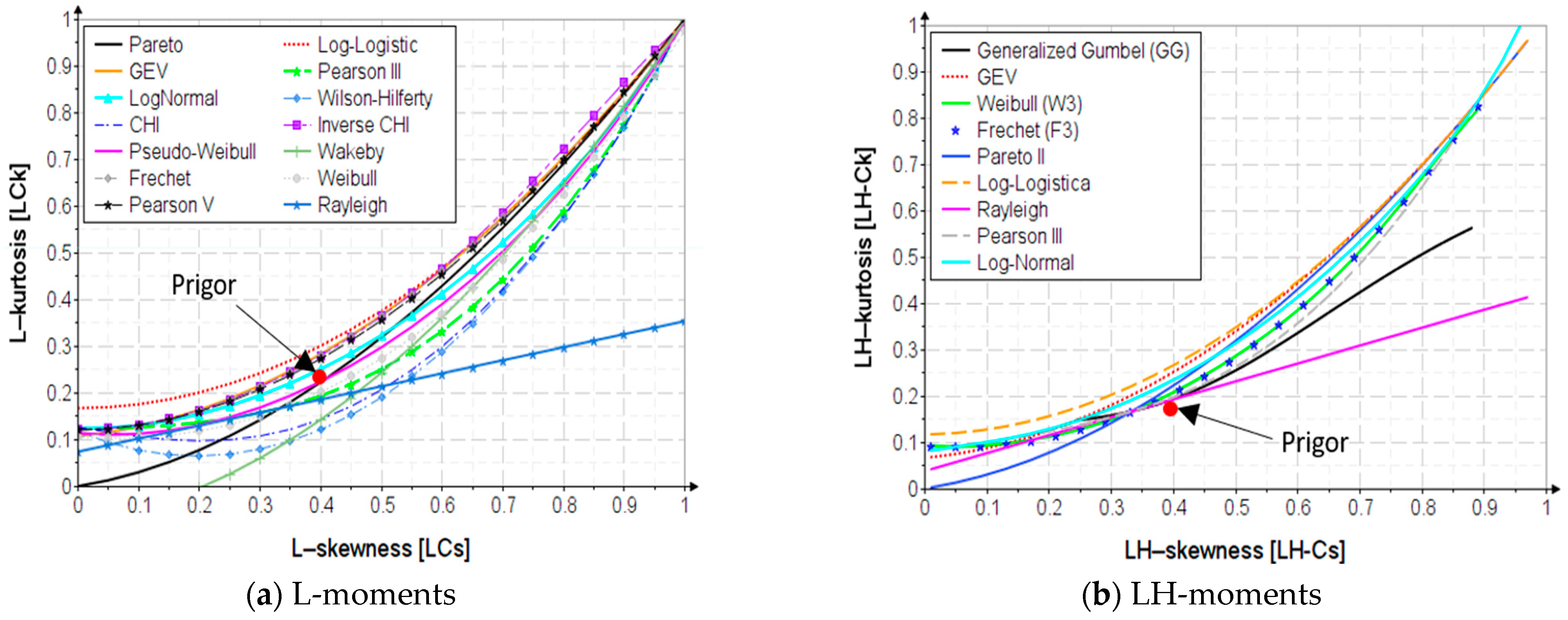
| The skewness-kurtosis variation graph and relationships | Raylegh | Pearson III, GEV, Weibull, log-normal, generalized Pareto, Raylegh, log-logistic |
| Distr. | Density Function | Complementary Cumulative Distribution Function | Inverse Function |
|---|---|---|---|
| PE3 | |||
| GEV | |||
| W3 | |||
| GP | |||
| RY | |||
| LN3 | |||
| LL3 |
| PG | |||||||
|---|---|---|---|---|---|---|---|
| Bias [%] | |||||||
| Statistical Indicators | Length (n) | Length (n) | |||||
| 1000 | 80 | 50 | 25 | 80 | 50 | 25 | |
| 1 | 0.998 | 0.997 | 0.994 | 0.2 | 0.3 | 0.6 | |
| 0.3 | 0.303 | 0.304 | 0.308 | −1 | −1.33 | −0.8 | |
| 0.3 | 0.303 | 0.305 | 0.309 | −1.09 | −1.64 | −2.91 | |
| 0.142 | 0.145 | 0.147 | 0.151 | −2.11 | −3.52 | −6.34 | |
| 1 | 0.986 | 0.981 | 0.97 | 1.4 | 1.9 | 3 | |
| 0.3 | 0.294 | 0.292 | 0.29 | 2 | 2.67 | 3.33 | |
| 0.5 | 0.488 | 0.485 | 0.482 | 2.4 | 2.91 | 3.69 | |
| 0.318 | 0.304 | 0.301 | 0.297 | 4.4 | 5.35 | 6.6 | |
| PG | |||||||
|---|---|---|---|---|---|---|---|
| Bias [%] | |||||||
| Parameters | Length (n) | Length (n) | |||||
| 1000 | 80 | 50 | 25 | 80 | 50 | 25 | |
| 0.077 | 0.069 | 0.065 | 0.056 | 10.39 | 15.58 | 27.27 | |
| 0.671 | 0.688 | 0.667 | 0.664 | 0.45 | 0.6 | 1.04 | |
| 0.377 | 0.373 | 0.371 | 0.365 | 1 | −1.62 | 3.18 | |
| −0.333 | −0.312 | −0.307 | −0.3 | 6.31 | 7.81 | 9.91 | |
| 0.333 | 0.337 | 0.337 | 0.335 | −1.2 | −1.2 | −0.6 | |
| 0.5 | 0.497 | 0.496 | 0.492 | 1 | −0.81 | 1.6 | |
| PG | |||||||
|---|---|---|---|---|---|---|---|
| Bias [%] | |||||||
| Annual Exceedance Probability [%] | Length (n) | Length (n) | |||||
| 1000 | 80 | 50 | 25 | 80 | 50 | 25 | |
| 0.01 | 4.81 | 4.92 | 4.99 | 5.14 | −2.48 | −3.75 | −6.89 |
| 0.1 | 3.97 | 4.04 | 4.08 | 4.17 | −1.74 | −2.64 | −4.83 |
| 0.5 | 3.30 | 3.34 | 3.36 | 3.41 | −1.21 | −1.82 | −3.34 |
| 1 | 2.98 | 3.01 | 3.02 | 3.06 | −0.97 | −1.48 | −2.69 |
| 0.01 | 21 | 18.5 | 18.0 | 17.1 | 12.07 | 14.69 | 18.91 |
| 0.1 | 9.5 | 8.7 | 8.5 | 8.2 | 8.14 | 10.04 | 13.26 |
| 0.5 | 5.3 | 5.1 | 5.0 | 4.8 | 5.52 | 6.92 | 9.41 |
| 1 | 4.1 | 4.0 | 3.9 | 3.8 | 4.44 | 5.65 | 7.82 |
| The AMS | ||||||||||||
|---|---|---|---|---|---|---|---|---|---|---|---|---|
| Year | 1990 | 1991 | 1992 | 1993 | 1994 | 1995 | 1996 | 1997 | 1998 | 1999 | 2000 | |
| Flow | [m3/s] | 9.96 | 15 | 10.1 | 14.8 | 7.30 | 21.2 | 18.2 | 21.4 | 13.1 | 14.5 | 35 |
| 2001 | 2002 | 2003 | 2004 | 2005 | 2006 | 2007 | 2008 | 2009 | 2010 | 2011 | ||
| Flow | [m3/s] | 19.9 | 22.1 | 11.8 | 80.3 | 88 | 51.6 | 72.2 | 16.2 | 42.6 | 28.5 | 12.8 |
| 2012 | 2013 | 2014 | 2015 | 2016 | 2017 | 2018 | 2019 | 2020 | ||||
| Flow | [m3/s] | 31.2 | 24.1 | 52.2 | 21.1 | 18.9 | 6.40 | 24.9 | 15.1 | 36.6 | ||
| Parameters | Distribution | ||||||
|---|---|---|---|---|---|---|---|
| PE3 | GEV | W3 | PG | RY | LN3 | LL3 | |
| L-moments | |||||||
| 0.6937 | −0.3277 | 0.848 | −0.1402 | −8.67 | 2.601 | 2.5083 | |
| 26.9 | 10.2 | 17.6 | 17.1 | 13.9 | 0.9569 | 20.3 | |
| 8.97 | 16.9 | 8.51 | 7.78 | 10.8 | 6.34 | 0.854 | |
| LH-moments | |||||||
| 0.5828 | −0.2708 | 0.8057 | −0.1496 | −14.9 | 2.8904 | 2.9638 | |
| 29.5 | 11.5 | 16.2 | 16.8 | 15.8 | 0.8078 | 27.2 | |
| 11.5 | 16.5 | 9.57 | 7.98 | 15.2 | 2.6013 | −5.95 | |
| Distr. | Annual Exceedance Probabilities [%] | |||||||||||||||||
|---|---|---|---|---|---|---|---|---|---|---|---|---|---|---|---|---|---|---|
| L-Moments | LH-Moments | |||||||||||||||||
| 0.01 | 0.1 | 0.5 | 1 | 2 | 3 | 5 | 80 | 90 | 0.01 | 0.1 | 0.5 | 1 | 2 | 3 | 5 | 80 | 90 | |
| PE3 | 231 | 172 | 130 | 113 | 95.4 | 85.3 | 72.7 | 11.4 | 9.80 | 239 | 176 | 133 | 114 | 96.3 | 85.8 | 72.8 | 13.1 | 12.0 |
| GEV | 623 | 285 | 163 | 127 | 97.7 | 83.6 | 68.2 | 12.4 | 9.50 | 489 | 250 | 152 | 122 | 96.3 | 83.5 | 69.0 | 11.4 | 7.90 |
| W3 | 249 | 180 | 134 | 115 | 96.2 | 85.6 | 72.5 | 11.5 | 9.75 | 264 | 188 | 138 | 117 | 97.5 | 86.3 | 72.7 | 12.1 | 10.6 |
| PG | 329 | 207 | 142 | 118 | 96.8 | 85.1 | 71.4 | 11.7 | 9.59 | 340 | 211 | 143 | 119 | 97.0 | 85.2 | 71.3 | 11.8 | 9.76 |
| RY | 229 | 170 | 130 | 112 | 95.0 | 85.0 | 72.6 | 11.2 | 9.72 | 242 | 178 | 134 | 115 | 96.9 | 86.3 | 73.2 | 12.2 | 11.6 |
| LN3 | 480 | 266 | 165 | 132 | 103 | 87.9 | 71.4 | 12.4 | 10.3 | 366 | 221 | 147 | 121 | 97.2 | 84.9 | 70.6 | 11.7 | 8.99 |
| LL3 | 800 | 320 | 168 | 128 | 96.7 | 82.1 | 66.6 | 12.5 | 9.31 | 603 | 274 | 157 | 123 | 95.3 | 82.1 | 67.6 | 11.1 | 7.03 |
| Distr. | Performance Measures | |||||||||||
|---|---|---|---|---|---|---|---|---|---|---|---|---|
| Methods for Parameter Estimation | Selection Criteria | |||||||||||
| L-Moments | LH-Moments | L-Moments | LH-Moments | |||||||||
| RME | RAE | RME | RAE | |||||||||
| PE3 | 0.0219 | 0.0885 | 0.399 | 0.192 | 0.0301 | 0.0953 | 0.398 | 0.197 | 0.399 | 0.228 | 0.398 | 0.177 |
| GEV | 0.0152 | 0.0636 | 0.282 | 0.0213 | 0.0925 | 0.250 | ||||||
| W3 | 0.0201 | 0.0822 | 0.202 | 0.0245 | 0.0850 | 0.206 | ||||||
| PG | 0.0181 | 0.0765 | 0.221 | 0.0187 | 0.0766 | 0.221 | ||||||
| RY | 0.0237 | 0.0955 | 0.185 | 0.0391 | 0.1133 | 0.192 | ||||||
| LN3 | 0.0199 | 0.0759 | 0.280 | 0.0148 | 0.0673 | 0.233 | ||||||
| LL3 | 0.0165 | 0.0715 | 0.299 | 0.0307 | 0.1204 | 0.265 | ||||||
| , | Annual Exceedance Probability [%] | |||
|---|---|---|---|---|
| P% | 0.01 | 0.1 | 0.5 | 1 |
| Bias [%] | 1.3 | 1.19 | 1.13 | 1.1 |
Disclaimer/Publisher’s Note: The statements, opinions and data contained in all publications are solely those of the individual author(s) and contributor(s) and not of MDPI and/or the editor(s). MDPI and/or the editor(s) disclaim responsibility for any injury to people or property resulting from any ideas, methods, instructions or products referred to in the content. |
© 2023 by the authors. Licensee MDPI, Basel, Switzerland. This article is an open access article distributed under the terms and conditions of the Creative Commons Attribution (CC BY) license (https://creativecommons.org/licenses/by/4.0/).
Share and Cite
Ilinca, C.; Stanca, S.C.; Anghel, C.G. Assessing Flood Risk: LH-Moments Method and Univariate Probability Distributions in Flood Frequency Analysis. Water 2023, 15, 3510. https://doi.org/10.3390/w15193510
Ilinca C, Stanca SC, Anghel CG. Assessing Flood Risk: LH-Moments Method and Univariate Probability Distributions in Flood Frequency Analysis. Water. 2023; 15(19):3510. https://doi.org/10.3390/w15193510
Chicago/Turabian StyleIlinca, Cornel, Stefan Ciprian Stanca, and Cristian Gabriel Anghel. 2023. "Assessing Flood Risk: LH-Moments Method and Univariate Probability Distributions in Flood Frequency Analysis" Water 15, no. 19: 3510. https://doi.org/10.3390/w15193510
APA StyleIlinca, C., Stanca, S. C., & Anghel, C. G. (2023). Assessing Flood Risk: LH-Moments Method and Univariate Probability Distributions in Flood Frequency Analysis. Water, 15(19), 3510. https://doi.org/10.3390/w15193510