
Ground Penetrating Radar Image Recognition for Earth Dam Disease Based on You Only Look Once v5s Algorithm


Abstract
:1. Introduction
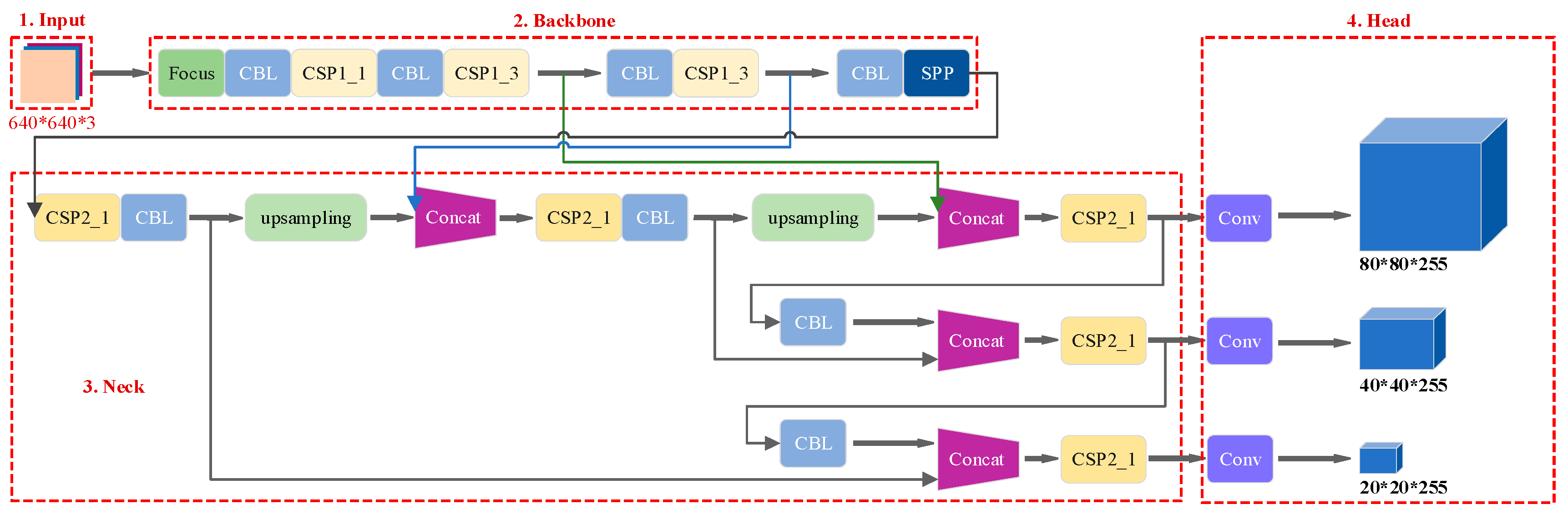
2. YOLOv5s Algorithm
- (1)
- Input
- (2)
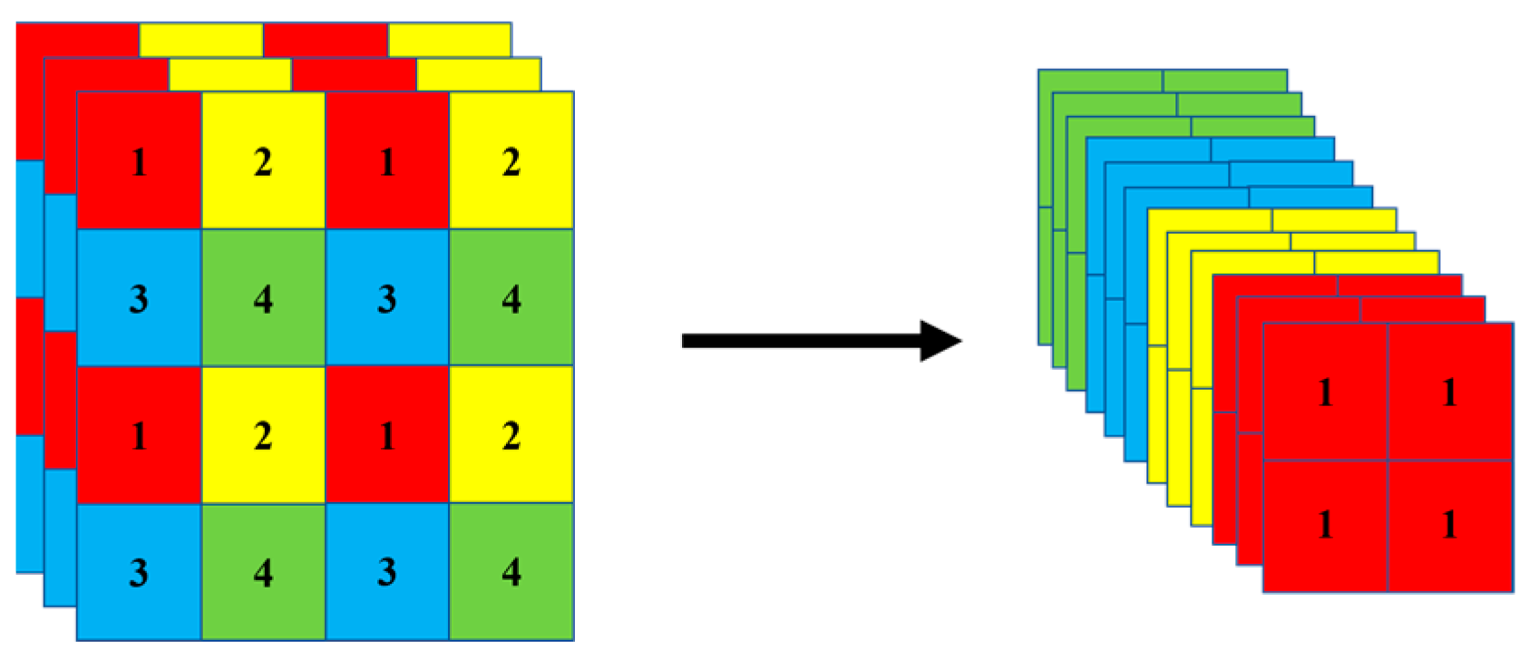
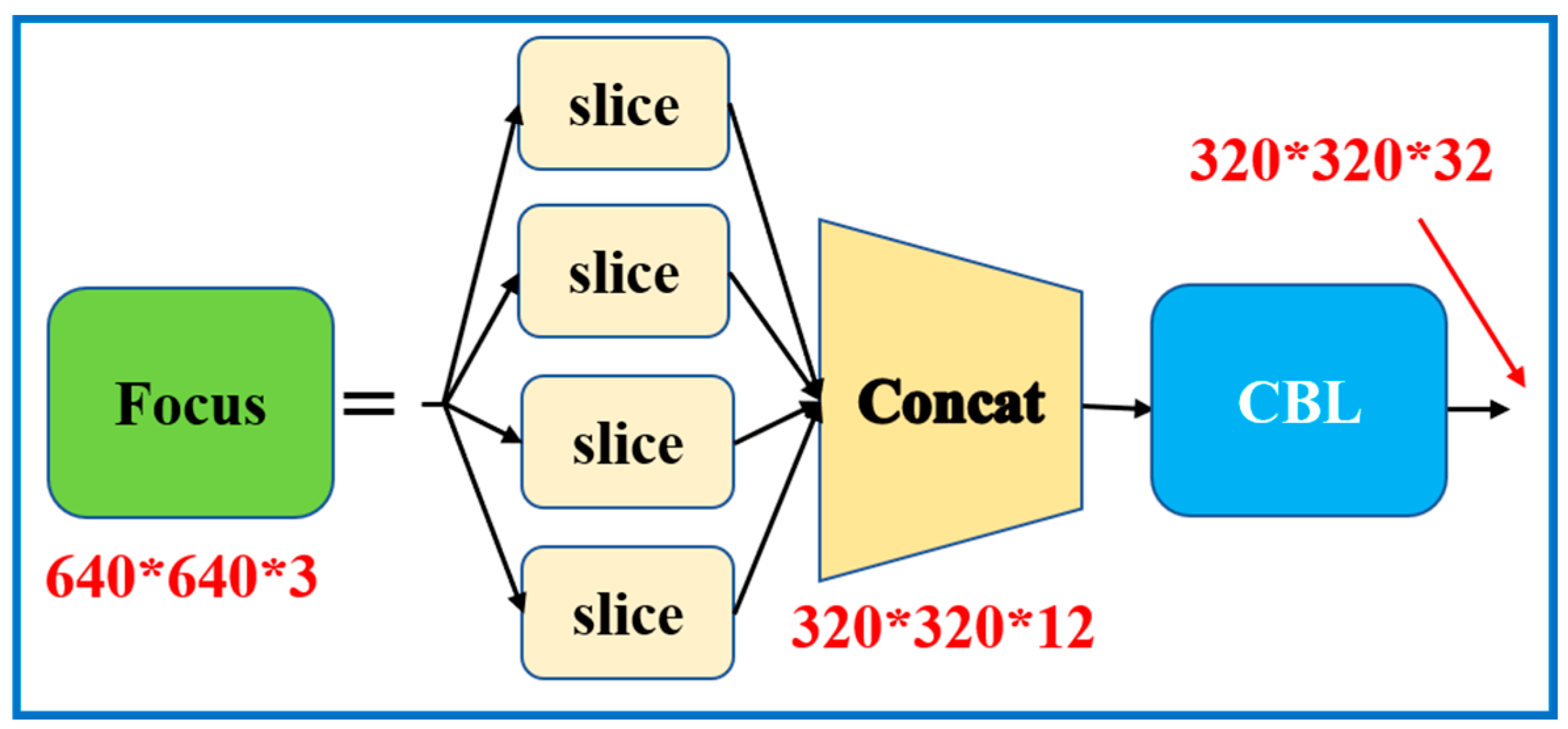
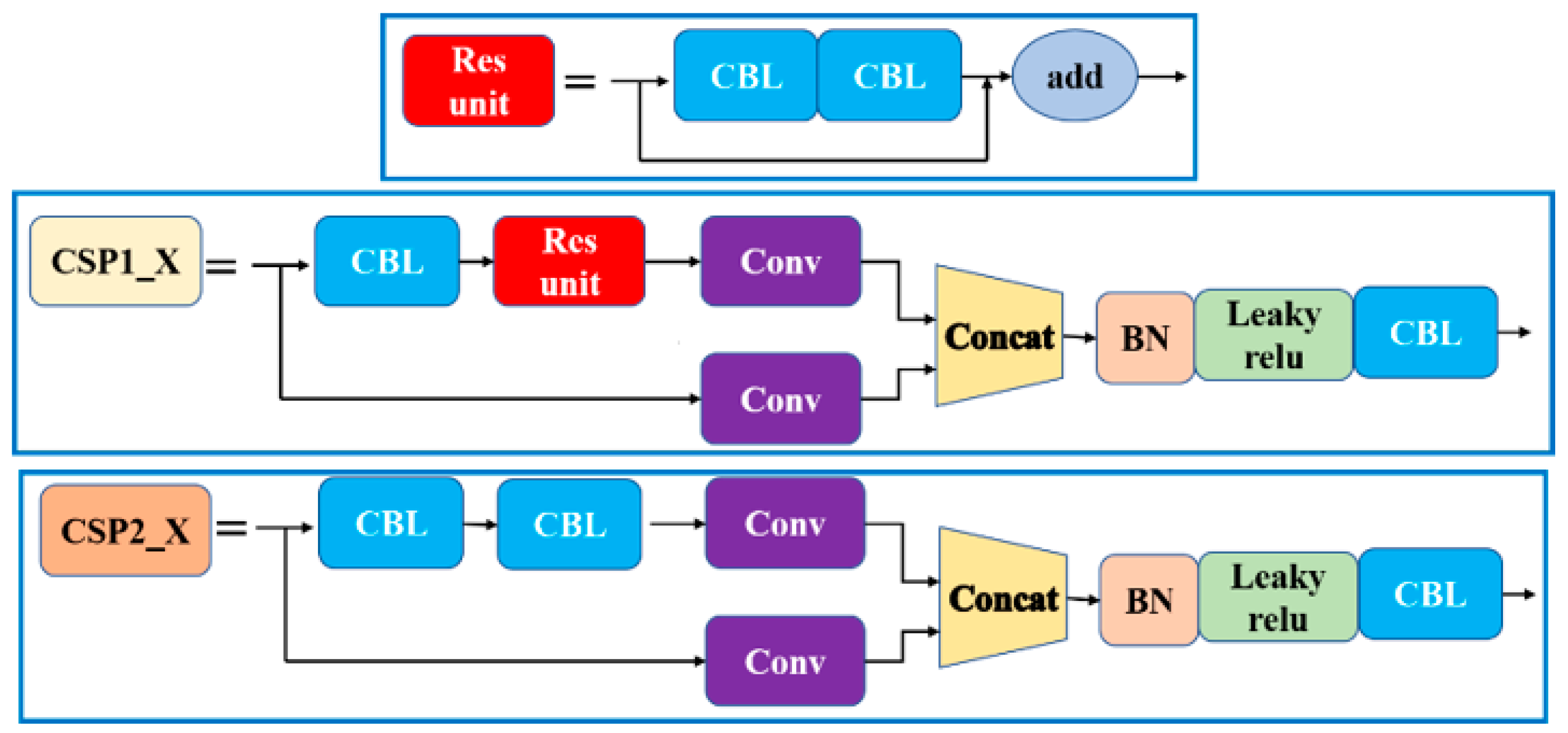
- Backbone
- (3)
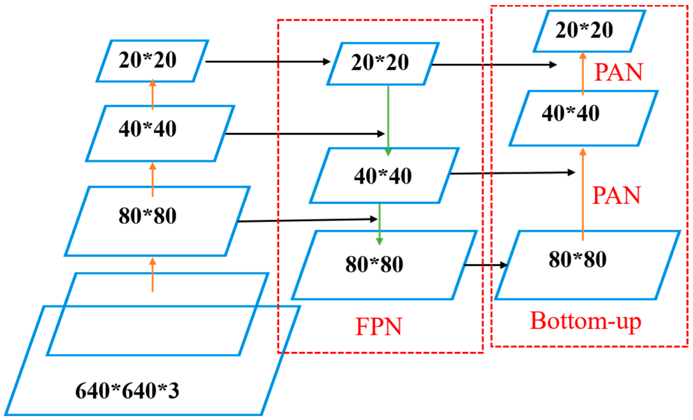
- Neck
- (4)
- Head
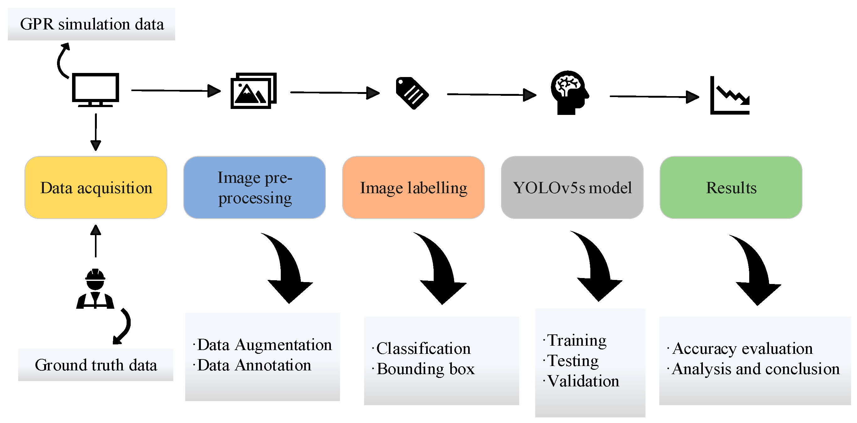
3. Construction of Earth Dam Disease Ground Penetrating Radar Dataset
3.1. Feature Data Acquisition
3.2. Data Augmentation
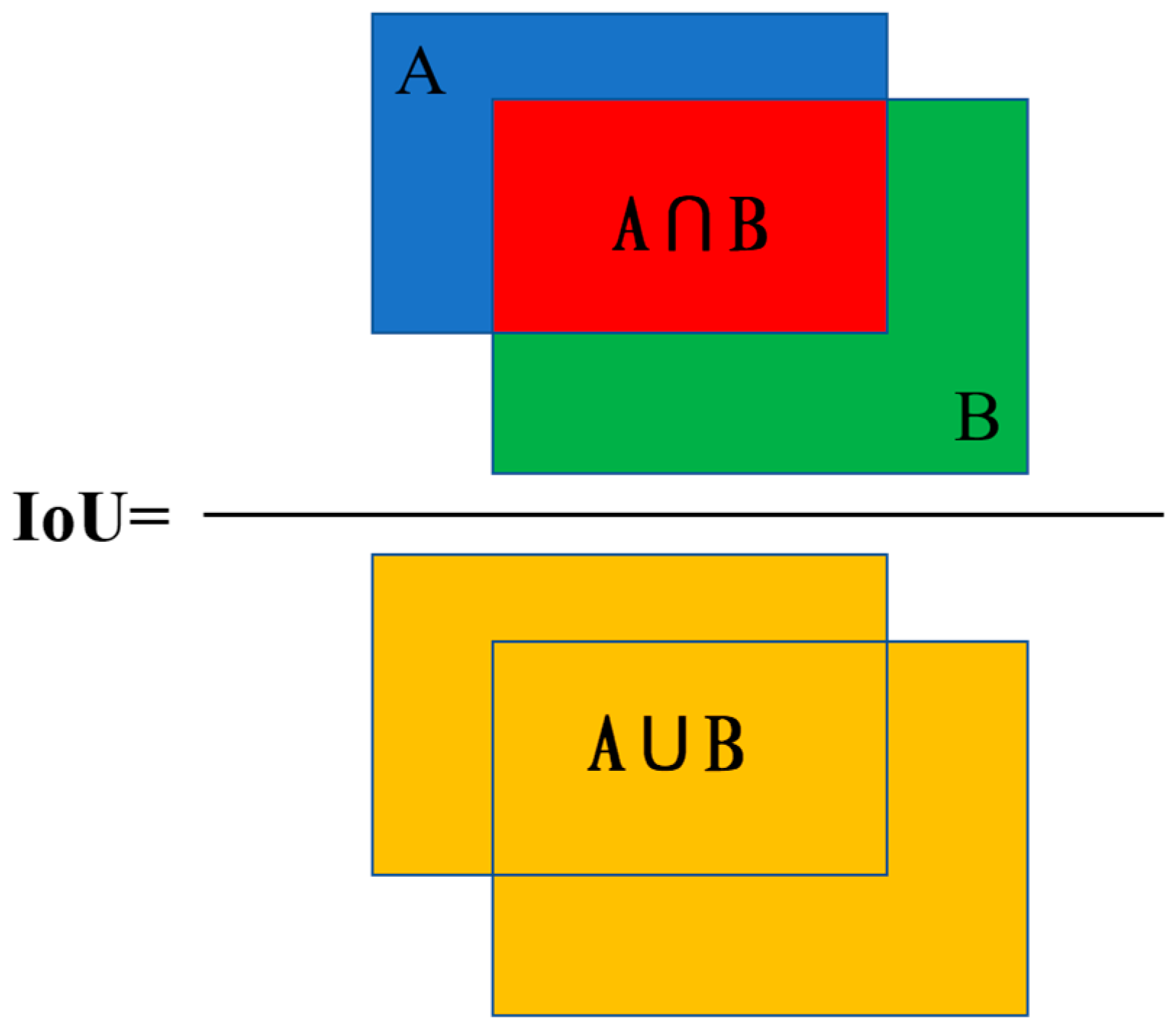
3.3. Data Annotation
4. Performance Evaluation Indicators
4.1. Evaluation Indicators
- (1)
- Accuracy (Acc) represents the proportion of samples correctly predicted by the earth dam disease detection model among all sample data. Although accuracy can judge the overall correctness, it cannot effectively measure the detection results in the case of imbalanced samples.
- (2)
- Precision (Pre) represents the proportion of correctly identified earth dam disease image samples among all samples identified as diseased, i.e., the accuracy rate of positive samples.
- (3)
- Recall (Rec) represents the proportion of images correctly identified as earth dam disease among all actual disease samples.
- (4)
- Average Precision (AP) equals the area enclosed by the P-R curve and the coordinate axis, representing the average value of the average precision for each category. Mean Average Precision (mAP) represents the average of the average precision APs for each category.
4.2. Loss Function
5. Model Training and Results Analysis
5.1. Training and Testing
5.2. Results Analysis
6. Conclusions
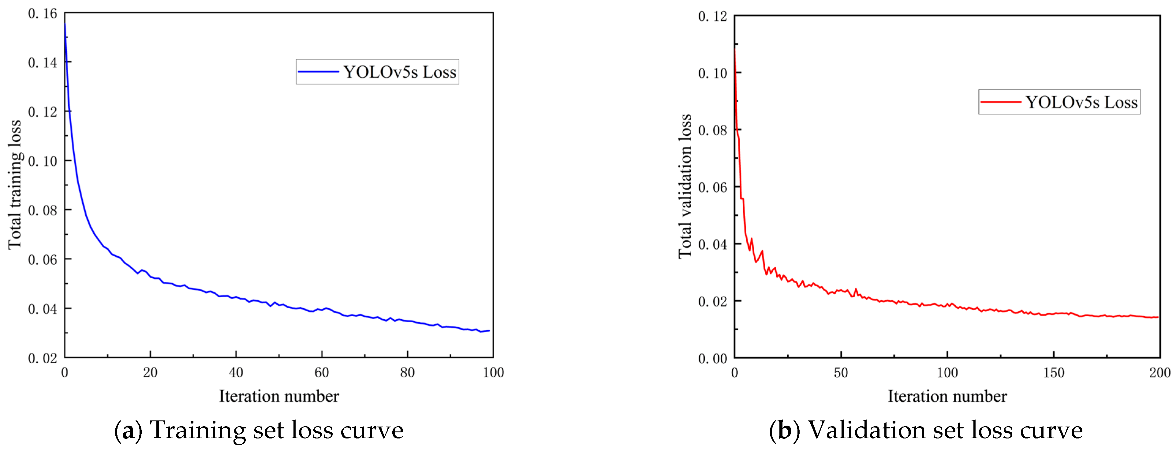
- (1)
- The YOLOv5s object detection model, when trained on the custom dataset, displays an initial decrease in the overall loss function followed by stabilization, with no signs of overfitting, demonstrating good generalization capability.
- (2)
- The average precision of the YOLOv5s object detection model varied for different earth dam diseases, with voids, seepage, and loosening diseases having average precision rates of 96.0%, 95.5%, and 93.9%, respectively.
- (3)
- The YOLOv5s object detection model can identify and classify earth dam disease ground-penetrating radar images, offering an effective method for intelligent detection of earth dam disease in practical engineering applications.
- (4)
- Considering that many factors affect the GPR field images, adding more GPR field images to train the target detection mode will improve the robustness of the model and build a more accurate target recognition model.
Author Contributions
Funding
Institutional Review Board Statement
Informed Consent Statement
Data Availability Statement
Conflicts of Interest
References
- Gołębiowski, T.; Piwakowski, B.; Ćwiklik, M.; Bojarski, A. Application of Combined Geophysical Methods for the Examination of a Water Dam Subsoil. Water 2021, 13, 2981. [Google Scholar] [CrossRef]
- Hu, S.; Lu, J.; Wang, G. Application analysis of detecting water-rich areas with ground-penetrating radar. Hydro-Sci. Eng. 2012, 6, 33–37. [Google Scholar]
- Gołębiowski, T.; Małysa, T. Application of GPR Method for Detection of Loose Zones in Flood Levee. E3S Web Conf. 2018, 30, 1008. [Google Scholar] [CrossRef]
- Marcak, H.; Golebiowski, T. The use of GPR attributes to map a weak zone in a river dike. Explor. Geophys. 2014, 45, 125–133. [Google Scholar] [CrossRef]
- Adamo, N.; Al-Ansari, N.; Sissakian, V.; Laue, J.; Knutsson, S. Geophysical Methods and their Applications in Dam Safety Monitoring. J. Earth Sci. Geotech. Eng. 2020, 11, 291–345. [Google Scholar] [CrossRef]
- Martínez-Pagán, P.; Gómez-Ortiz, D.; Martín-Crespo, T.; Martín-Velázquez, S.; Martínez-Segura, M. Electrical Resistivity Imaging Applied to Tailings Ponds: An Overview. Mine Water Environ. 2021, 40, 285–297. [Google Scholar] [CrossRef]
- Neyamadpour, A.; Abbasinia, M. Application of electrical resistivity tomography technique to delineate a structural failure in an embankment dam: Southwest of Iran. Arab. J. Geosci. 2019, 12, 420. [Google Scholar] [CrossRef]
- Shin, S.; Park, S.; Kim, J.-H. Time-lapse electrical resistivity tomography characterization for piping detection in earthen dam model of a sandbox. J. Appl. Geophys. 2019, 170, 103834. [Google Scholar] [CrossRef]
- Loperte, A.; Soldovieri, F.; Lapenna, V. Monte Cotugno Dam Monitoring by the Electrical Resistivity Tomography. IEEE J. Sel. Top. Appl. Earth Obs. Remote Sens. 2015, 8, 5346–5351. [Google Scholar] [CrossRef]
- Hui, L.; Haitao, M. Application of Ground Penetrating Radar in Dam Body Detection. Procedia Eng. 2011, 26, 1820–1826. [Google Scholar] [CrossRef]
- Vonnisa, M.; Shimomai, T.; Hashiguchi, H.; Marzuki, M. Retrieval of Vertical Structure of Raindrop Size Distribution from Equatorial Atmosphere Radar and Boundary Layer Radar. Emerg. Sci. J. 2022, 6, 448–459. [Google Scholar] [CrossRef]
- Dong, Z.; Xue, B.; Lei, J.; Zhao, X.; Gao, J. Study on Propagation Characteristics of Ground Penetrating Radar Wave in Dikes and Dams with Polymer Grouting Repair Using Finite-Difference Time-Domain with Perfectly Matched Layer Boundary Condition. Sustainability 2022, 14, 10293. [Google Scholar] [CrossRef]
- Lin, T.; Goyal, P.; Girshick, R.; He, K.; Dollár, P. Focal loss for dense object detection. In Proceedings of the IEEE International Conference on Computer Vision (ICCV), Venice, Italy, 22–29 October 2017; pp. 2999–3007. [Google Scholar]
- Ren, S.; He, K.; Girshick, R.; Sun, J. Faster R-CNN: Towards real-time object detection with region proposal networks. IEEE Trans. Pattern Anal. Mach. Intell. 2015, 39, 1137–1149. [Google Scholar] [CrossRef]
- Redmon, J.; Divvala, S.; Girshick, R.; Farhadi, A. You Only Look Once: Unified, Real-Time Object Detection. In Proceedings of the 2016 IEEE Conference on Computer Vision and Pattern Recognition (CVPR), Las Vegas, NV, USA, 27–30 June 2016; IEEE: Piscataway, NJ, USA, 2016; pp. 779–788. [Google Scholar] [CrossRef]
- Haque, I.; Alim, M.; Alam, M.; Nawshin, S.; Noori, S.R.H.; Habib, T. Analysis of Recognition Performance of Plant Leaf Diseases Based on Machine Vision Techniques. J. Human Earth Future 2022, 3, 129–137. [Google Scholar] [CrossRef]
- Redmon, J.; Farhadi, A. YOLO9000: Better, Faster, Stronger. In Proceedings of the 30th IEEE Conference on Computer Vision and Pattern Recognition, Honolulu, HI, USA, 21–26 July 2017; pp. 6517–6525. [Google Scholar] [CrossRef]
- Redmon, J.; Farhadi, A. YOLOv3: An Incremental Improvement. arXiv 2018, arXiv:1804.02767. [Google Scholar]
- Bochkovskiy, A.; Wang, C.; Liao, H.M. YOLOv4: Optimal Speed and Accuracy of Object Detection. arXiv 2020, arXiv:2004.10934. [Google Scholar]
- Jocher, G.R.; Stoken, A.; Borovec, J.I.; Chaurasia, A.; Changyu, L.; Hogan, A.; Hajek, J.; Diaconu, L.; Kwon, Y.; Defretin, Y.; et al. ultralytics/yolov5: v5.0—YOLOv5-P6 1280 models, AWS, Supervise.ly and YouTube integrations. 2021. Available online: https://api.semanticscholar.org/CorpusID:244964519 (accessed on 26 May 2022).
- Li, C.; Li, L.; Jiang, H.; Weng, K.; Geng, Y.; Li, L.; Ke, Z.; Li, Q.; Cheng, M.; Nie, W.; et al. YOLOv6: A Single-Stage Object Detection Framework for Industrial Applications. arXiv 2022, arXiv:2209.02976. [Google Scholar]
- Wang, C.-Y.; Bochkovskiy, A.; Liao, H.-Y.M. YOLOv7: Trainable Bag-of-Freebies Sets New State-of-the-Art for Real-Time Object Detectors. In Proceedings of the 2023 IEEE/CVF Conference on Computer Vision and Pattern Recognition (CVPR), Vancouver, BC, Canada, 17–24 June 2023; IEEE: Piscataway, NJ, USA, 2023; pp. 7464–7475. [Google Scholar] [CrossRef]
- Zhu, X.; Lyu, S.; Wang, X.; Zhao, Q. TPH-YOLOv5: Improved YOLOv5 Based on Transformer Prediction Head for Object Detection on Drone-captured Scenarios. In Proceedings of the 2021 IEEE/CVF International Conference on Computer Vision Workshops (ICCVW 2021), Montreal, BC, Canada, 11–17 October 2021; IEEE: Piscataway, NJ, USA, 2021; pp. 2778–2788. [Google Scholar] [CrossRef]
- Kurdthongmee, W.; Kurdthongmee, P.; Suwannarat, K.; Kiplagat, J.K. A YOLO Detector Providing Fast and Accurate Pupil Center Estimation using Regions Surrounding a Pupil. Emerg. Sci. J. 2022, 6, 985–997. [Google Scholar] [CrossRef]
- Yan, B.; Fan, P.; Lei, X.; Liu, Z.; Yang, F. A Real-Time Apple Targets Detection Method for Picking Robot Based on Improved YOLOv5. Remote Sens. 2021, 13, 1619. [Google Scholar] [CrossRef]
- Wang, S.; Chen, X.; Dong, Q. Detection of Asphalt Pavement Cracks Based on Vision Transformer Improved YOLO V5. J. Transp. Eng. Part B Pavements 2023, 149, 04023004. [Google Scholar] [CrossRef]
- Sozzi, M.; Cantalamessa, S.; Cogato, A.; Kayad, A.; Marinello, F. Automatic Bunch Detection in White Grape Varieties Using YOLOv3, YOLOv4, and YOLOv5 Deep Learning Algorithms. Agronomy 2022, 12, 319. [Google Scholar] [CrossRef]
- Terven, J.; Cordova-Esparza, D. A Comprehensive Review of YOLO: From YOLOv1 to YOLOv8 and Beyond. arXiv 2023, arXiv:2304.00501. [Google Scholar]
- Jiang, Z.; Zeng, Z.; Li, J.; Liu, F.; Li, W. Simulation and analysis of GPR signal based on stochastic media model with an ellipsoidal autocorrelation function. J. Appl. Geophys. 2013, 99, 91–97. [Google Scholar] [CrossRef]
- Rezatofighi, H.; Tsoi, N.; Gwak, J.; Sadeghian, A.; Reid, I.; Savarese, S. Generalized Intersection Over union: A metric and a Loss for Bounding Box Regression. In Proceedings of the 2019 IEEE/CVF Conference on Computer Vision and Pattern Recognition (CVPR 2019), Long Beach, CA, USA, 15–20 June 2019; IEEE: Piscataway, NJ, USA, 2019; pp. 658–666. [Google Scholar] [CrossRef]
- Xue, J.; Cheng, F.; Li, Y.; Song, Y.; Mao, T. Detection of Farmland Obstacles Based on an Improved YOLOv5s Algorithm by Using CIoU and Anchor Box Scale Clustering. Sensors 2022, 22, 1790. [Google Scholar] [CrossRef]


Disclaimer/Publisher’s Note: The statements, opinions and data contained in all publications are solely those of the individual author(s) and contributor(s) and not of MDPI and/or the editor(s). MDPI and/or the editor(s) disclaim responsibility for any injury to people or property resulting from any ideas, methods, instructions or products referred to in the content. |
© 2023 by the authors. Licensee MDPI, Basel, Switzerland. This article is an open access article distributed under the terms and conditions of the Creative Commons Attribution (CC BY) license (https://creativecommons.org/licenses/by/4.0/).
Share and Cite
Xue, B.; Gao, J.; Hu, S.; Li, Y.; Chen, J.; Pang, R. Ground Penetrating Radar Image Recognition for Earth Dam Disease Based on You Only Look Once v5s Algorithm. Water 2023, 15, 3506. https://doi.org/10.3390/w15193506
Xue B, Gao J, Hu S, Li Y, Chen J, Pang R. Ground Penetrating Radar Image Recognition for Earth Dam Disease Based on You Only Look Once v5s Algorithm. Water. 2023; 15(19):3506. https://doi.org/10.3390/w15193506
Chicago/Turabian StyleXue, Binghan, Jianglin Gao, Songtao Hu, Yan Li, Jianguo Chen, and Rui Pang. 2023. "Ground Penetrating Radar Image Recognition for Earth Dam Disease Based on You Only Look Once v5s Algorithm" Water 15, no. 19: 3506. https://doi.org/10.3390/w15193506
APA StyleXue, B., Gao, J., Hu, S., Li, Y., Chen, J., & Pang, R. (2023). Ground Penetrating Radar Image Recognition for Earth Dam Disease Based on You Only Look Once v5s Algorithm. Water, 15(19), 3506. https://doi.org/10.3390/w15193506