Article

An Integration of Geospatial Modelling and Machine Learning Techniques for Mapping Groundwater Potential Zones in Nelson Mandela Bay, South Africa

Department of Geography Archaeology and Environmental Studies, University of Witwatersrand, Johannesburg 2000, South Africa
*
Author to whom correspondence should be addressed.
Water 2023, 15(19), 3447; https://doi.org/10.3390/w15193447
Submission received: 7 July 2023 / Revised: 29 August 2023 / Accepted: 30 August 2023 / Published: 30 September 2023
(This article belongs to the Section Hydrology)

Abstract

:
Groundwater is an important element of the hydrological cycle and has increased in importance due to insufficient surface water supply. Mismanagement and population growth have been identified as the main drivers of water shortage in the continent. This study aimed to derive a groundwater potential zone (GWPZ) map for Nelson Mandela Bay (NMB) District, South Africa using a geographical information system (GIS)-based analytic hierarchical process (AHP) and machine learning (ML) random forest (RF) algorithm. Various hydrological, topographical, remote sensing-based, and lithological factors were employed as groundwater-controlling factors, which included precipitation, land use and land cover, lineament density, topographic wetness index, drainage density, slope, lithology, and soil properties. These factors were weighted and scaled by the AHP technique and their influence on groundwater potential. A total of 1371 borehole samples were divided into 70:30 proportions for model training (960) and model validation (411). Borehole location training data with groundwater factors were incorporated into the RF algorithm to predict GWPM. The model output was validated by the receiver-operating characteristic (ROC) curve, and the models’ reliability was assessed by the area under the curve (AUC) score. The resulting groundwater-potential maps were derived using a weighted overlay for AHP and RF models. GWPM computed using weighted overlay classified groundwater potential zones (GWPZs) as having low (2.64%), moderate (29.88%), high (59.62%) and very high (7.86%) groundwater potential, whereas GWPZs computed using RF classified GWPZs as having low (0.05%), moderate (31.00%), high (62.80%) and very high (6.16%) groundwater potential. The RF model showed superior performance in predicting GWPZs in Nelson Mandela Bay with an AUC score of 0.81 compared to AHP with an AUC score of 0.79. The results reveal that Nelson Mandela Bay has high groundwater potential, but there is a water supply shortage, partially caused by inadequate planning, management, and capacity in identifying potential groundwater zones.

1. Introduction

Water scarcity has been identified as a major issue, especially in developing nations where there are insufficient exploration methods and inadequate water supply to meet the population demand [1]. South Africa has recorded inadequate water distribution with a sharp increase in water shortage [2], where provinces such as Eastern Cape have declared a surge in water demand since municipalities were confronted with the challenge of meeting water users’ demands. Since surface water faces many challenges, including availability, scientists have revealed that groundwater could play a significant role in meeting water users’ demands.
Groundwater, which is usually defined as the water that exists in the pore spaces of rock or soil [3], represents about 30% of the globe’s freshwater [4] and has a vital function in the hydrological cycle [5], especially in areas with limited access to freshwater, where it serves as vital freshwater for both urban and rural communities. Groundwater normally exists in the saturated zone where pore spaces are mostly filled with water. The unsaturated zone (vadose zone) is where pore spaces are filled with both air water [6], where not all pore spaces are filled with water. Groundwater is less subject to climate change and has been shown to be an affordable choice for agriculture, industrial, domestic, and other uses [7]. However, groundwater is little utilized in most African countries due to its operational costs, limited access to technology, lack of infrastructure, and lack of knowledge in terms of its occurrence [8]. Africa possesses a substantial groundwater storage capacity, which is roughly calculated to be 100 times more extensive than available renewable freshwater and about 20 times larger than the water held in the surface dams or lakes [9]. The potential of groundwater storage in Africa presents an opportunity to address the continent’s water scarcity issues and underscores the importance of effective management and sustainable use of this valuable resource [8].
The management and utilization of groundwater require a proper method that measures its quality, quantity and spatial variability, and these measures ensure groundwater sustainability [10]. Extensive extraction of groundwater can lead to a decrease in the groundwater level [11], and consequently, effective groundwater monitoring is essential in areas where groundwater plays a central role in the local water supply: “Groundwater mapping serves as an indicator of the variability of groundwater throughout the region and the likelihood of their presence” [6]. History has revealed that researchers have concentrated on in situ measurements of groundwater potential mapping (GWPM), which are frequently too expensive, time-consuming and impractical for large regional-scale research [12]. These approaches to groundwater exploration include drilling, geophysics and hydrogeological methods [10,13]. Although these methods were often too expensive and time-consuming, they gave accurate and reliable results. As a result, Fajana [14] attempted to delineate groundwater aquifer potential in Odo Ayedun in Nigeria based on electric resistivity and porosity calculations, where they carried out a reconnaissance survey of the study area to acquire coordinates and interpret vertical electric sounding data for subsurface geology. The traditional methods have helped researchers in achieving aims that pertain to groundwater delineation and have revealed a vital function in recognizing prospective areas for borehole excavation: “The lack of adequate technology in identifying the groundwater potential zones and proper planning remains to be a bottleneck in developing continents” [6], especially in Africa [8].
As technology advances, researchers have proved geographical information systems (GISs) and remote sensing (RS) to be more affordable and effective methods in GWPM for sustainable planning, administration, and management of aquifers [11], since these methods provide an ability to generate complex hydrological content for the spatiotemporal domain [15] with crucial spatial analysis and predictive modelling equipment. Remote sensing satellites often do not provide the details of groundwater variability by penetrating deeply through the subsurface soil and geological media. Rather, they assist in explaining features that could be associated with the availability of groundwater [16]. The GIS approach has been integrated with various techniques, such as multicriteria decision-making methods including analytical hierarchical process (AHP) which is widely used for groundwater mapping [2,5,8,17], and fuzzy-AHP [18,19], multi-influencing factor (MIF), fuzzy logic (FL), certainty factor (CF) [20], weight of evidence (WOE) [21], evidence belief function (EBF) [22] for landslide mapping, and index models (IMs) [17,23]. Other researchers, such as Mogaji et al. [24], have also attempted to delineate GWPZs based on techniques such as the Dempster–Shafer theory of evidence (DS-EBF) model, which revealed great accuracy.
The AHP technique, as explained by Abrar et al. [8], enables researchers to define groundwater potential zones (GWPZs) by evaluating the importance of hierarchically non-saturated criteria concerning those positioned at a high level. Based on the AHP and GIS approach, Ndhlovu et al. [17] evaluated GWPZs in the Zambezi by assessing the effect of various factors, such as lineament density, lithology, land use and land cover (LULC), soil properties, slope degrees, rainfall, and drainage density, and argued that these factors have the potential in determining groundwater potential. Owolabi [25] attempted to develop feasible research to demonstrate a GWPZ with a high accuracy in the Eastern Cape, and claimed that the AHP model is vital to delineating GWPZs in semiarid regions. Gintamo [15] applied GIS-based integrated Saaty’s AHP to derive GWPZs in Ethiopia’s Bilate River Catchment by assessing the extent of impact and contribution of each factor to groundwater potential. Moodley et al. [5] attempted to delineate GWPZs in KwaZulu Natal (KZN), South Africa based on the AHP approach, claimed their study was the first to establish GWPZs in KZN through an integration of GIS, remote sensing and AHP techniques, and contended that the procedure of delineating GWPZs in South Africa is largely characterized by obsolete, time-intensive, and expensive in situ methods [6].
Technological progress has shifted towards machine learning (ML) and deep learning (DL), and recent studies have employed these algorithms to accurately derive GWPZs [10,26,27] and improve model accuracy and efficiency [28]. The ML and DL techniques rely heavily on the availability and quality of the dataset [29] since these techniques learn from experience and identify hidden patterns [30]. Researchers have demonstrated the efficiency of ML and DL algorithms in various applications including landslide susceptibility mapping, floods, and groundwater prediction [6]. There are various types of ML algorithms developed by researchers thus far, including support vector machine (SVM), random forest (RF), boosted regression tree (BRT), classification regression tree (CRT), naïve Bayes (NB), and DL algorithms, including convolutional neural network (CNN), artificial neural network (ANN), recurrent neural network (RNN) and long short-term memory (LSTM) [6,10,11,31]. For groundwater mapping, researchers have proved the efficiency of the ML and DL algorithms BRT, RF and SVM [11], RF [27,32], CNN and SVM [33], logistic regression [34], classification and regression tree (CART) [35], naïve Bayes [27], and LSTM [10] for groundwater prediction. These techniques have allowed researchers to improve their performance through the process of hybrid or model ensembles. Arabameri et al. [7] employed a new hybrid model that combined random subspace and multilayer perception (MLP) and achieved very high accuracy. Studies such as Hasanuzzaman et al. [27] have demonstrated the capability of ML by comparing RF with multicriteria AHP, where RF derived GWPZs with high accuracy. Moreover, these techniques still require in situ measurement as an appropriate method of model accuracy validation.
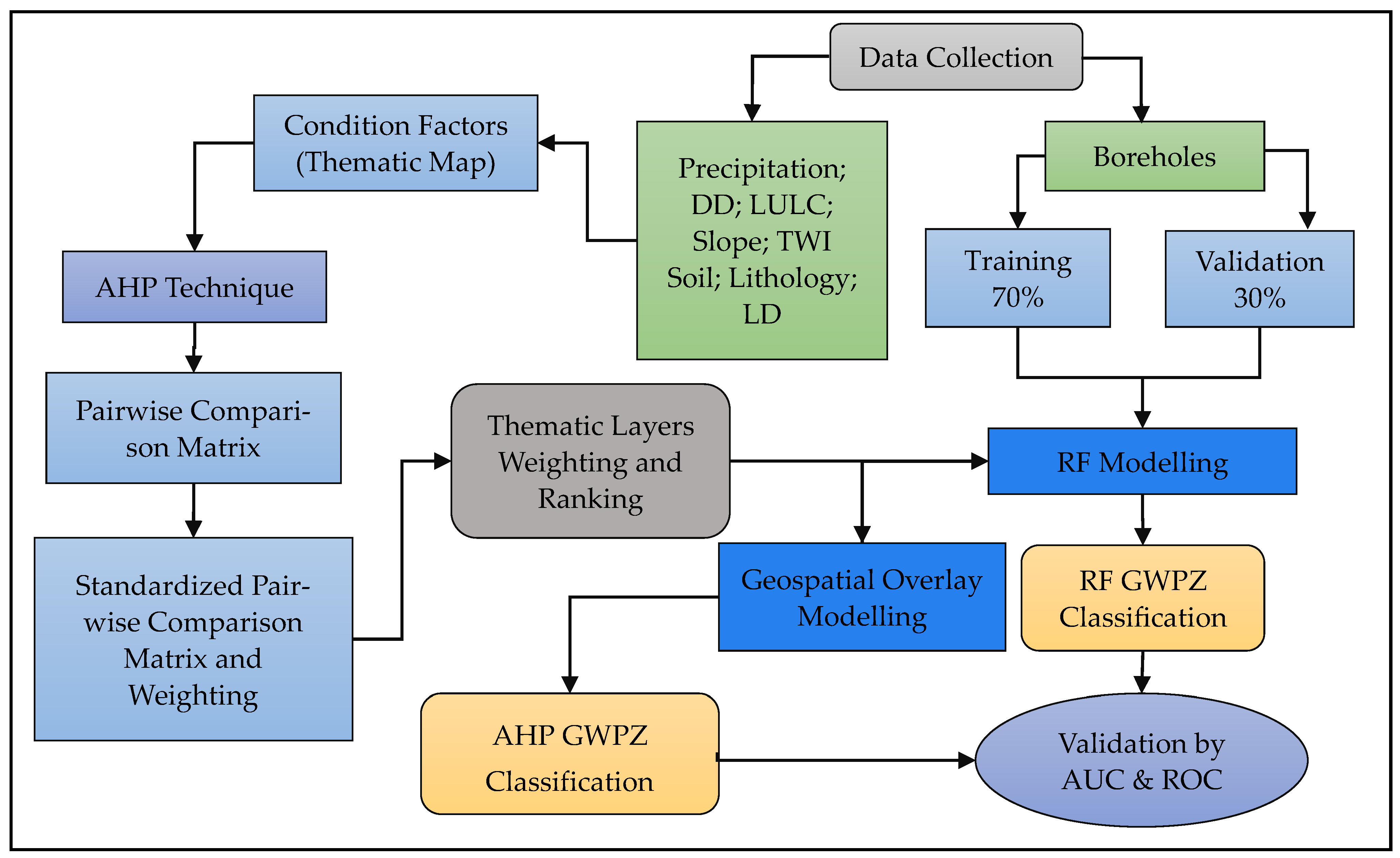
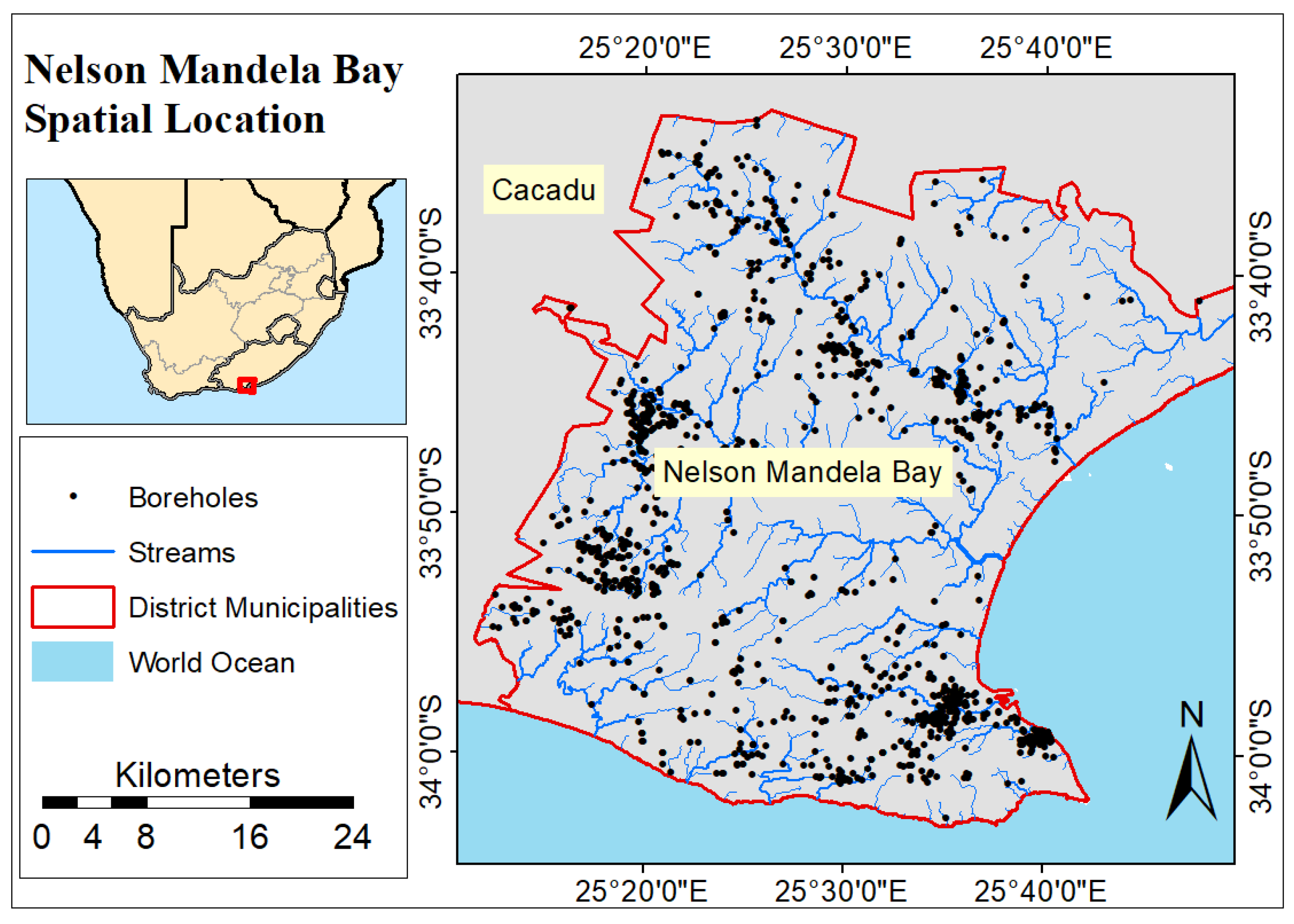
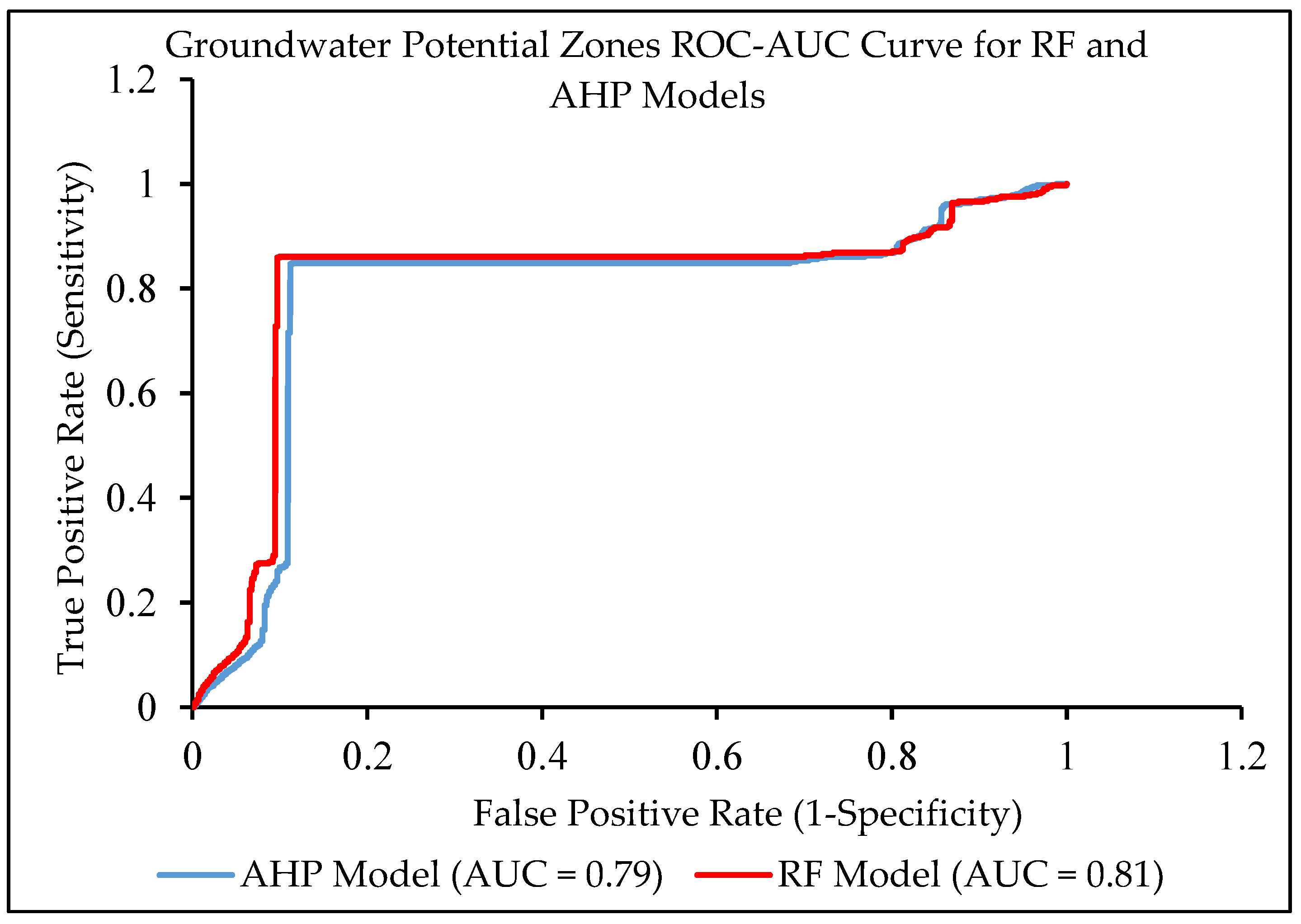
Despite these promising techniques for assessing groundwater resources, the spatial variation of aquifers is recognized at the national level in South Africa, but less is known about the specific case of Nelson Mandela Bay (NMB). Hence, the main objective of this study was to delineate a groundwater potential zone map for Nelson Mandela Bay, South Africa by integrating geographical information system, analytic hierarchical process, and machine learning-based random forest models. The AHP technique was employed to identify optimal parameters and assign weightage to criteria for groundwater potential zone (GWPZ) assessment. The area under the receiver-operating characteristic curve (AU-ROC) was utilized to assess the performance of both the AHP and RF groundwater prediction algorithms. The study also mapped the spatial distribution of groundwater in the NMB region. The groundwater potential zone map derived from this study is anticipated to play a significant role in informing policymakers, water managers, and other stakeholders involved in managing and preserving the region’s groundwater resources, contributing to the long-term resilience and sustainability of South Africa’s water systems.
The introduction of this study provides an overview of the study area and sets forth the study objectives. We explore materials and methods to detail the approach to delineate groundwater potential mapping starting with the preparation of thematic factors. We then apply the AHP technique to compute the weight and ranking of these factors, followed by the construction of a weighted overlay model to generate an initial groundwater map. The RF model enhances the accuracy and robustness of groundwater prediction. Section 3 showcases the spatial variability of thematic factors and the delineated groundwater potential zones. The model validation and comparison derive which model was most efficient. Finally, the discussion highlights the interpretation of the findings and their implications, while the conclusion summarizes the key outcomes and suggests future research directions.

Overview of the Study Area

Nelson Mandela Bay (NMB) Metropolitan is a vibrant coastal city situated in the Eastern Cape province of South Africa, covering an approximate area of 1959   km 2 with its central coordinates marked as 33°48′ S, 25°30′ E, as presented in Figure 1. NMB is situated on the shores of the Indian Ocean and has a diverse culture and heritage, making it a popular tourist destination, and it is considered an economic giant in the country. NMB lies within a transitional climatic region, characterized by a blend of climatic influence from the KZN summer rainfall and the Western Cape Mediterranean climate [6,36]. The positioning of NMB between these climatic regions results in distinct weather patterns and conditions. It features a warm-temperature climate, characterized by an average annual temperature of approximately 22 °C and an average annual rainfall of 490   mm . “The southern half of the district is dominated by fractured rocks, which consist of the Table Mountain group” [6] (shale), Bokkeveld Group (shale and limestone), and a weak rock of the Uitenhage Group (sandstone) [37].
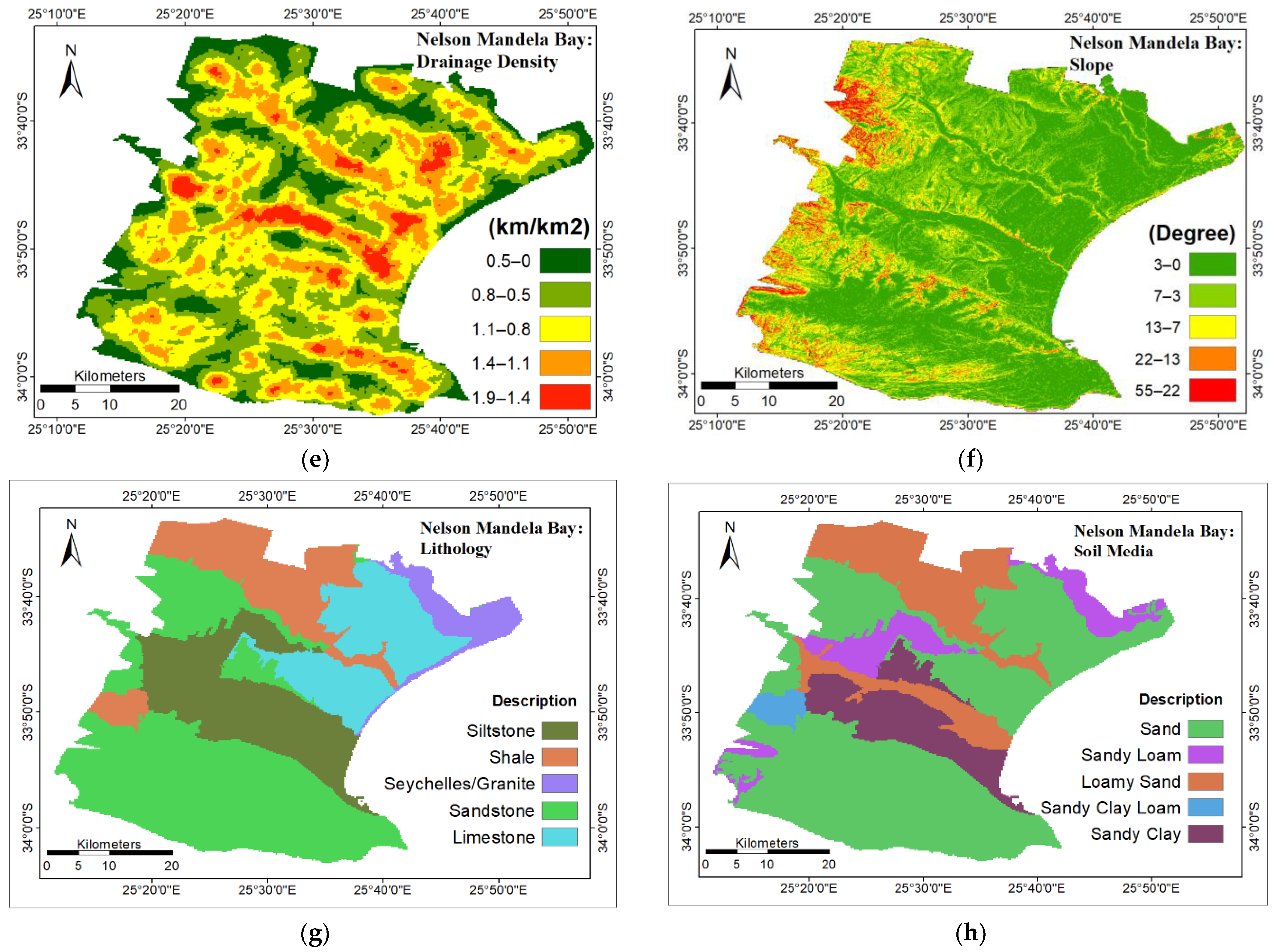
The district’s lithology consists of shale, sandstone, siltstone, limestone, and granite. The eastern coastline of the district is characterized by a cape fold belt comprising fine-grained quartzites derived from Table Mountain’s sandstone [36]. The soil composition in NMB predominantly consists of Nanaga coastal formation, sandy loam soil, sandy clay, loamy sand and sandy clay loam. Additionally, the upper Swartkops regions hold agricultural significance due to their favorable soil characteristics [6,36]. NMB encompasses extensive forested areas, sparsely vegetated regions, and agriculturally active zones, with 25% of the total area occupied by surface water bodies. The topography of the district is shaped by marine strata filling a wide valley at the terminus of the east–west-oriented Cape Fold Belt. The predominant topographical features consist of flat and gradually sloping areas towards the sea. This configuration is likely influenced by a blend of marine and continental erosion processes [36]. The mountains protrude in the western boundary of the district.

2. Materials and Methods

2.1. Methodological Approach

The research was segmented into four distinct phases: the initial phase was selecting and evaluating parameters, weighting and rating for GWPZ modelling; the second phase was to develop the geospatial model for GWPZ delineation; the third phase was to compare the efficiency of AHP and RF for GWPZ modelling through the area under the receiver operating characteristic curve; and the fourth phase was to generate a groundwater distribution map for NMB.
This study adopted a methodological approach followed by other studies [5,31,38], presented in Figure 2. This study employed parameters that are frequently utilized in other research studies, which encompass drainage density, precipitation, land use and land cover (LULC), slope and topographic wetness index (TWI). Secondary data sources such as soil texture, lithological properties, lineament density and borehole location were also included. Other studies have used various parameters for ML algorithms including aspect, distance from rivers, distance from the fault lines, profile and plan curvature [10,31]. The present study initially employed the AHP technique to delineate GWPZs through a process of weighted overlay analysis. By extracting the value of GWPZs from boreholes and parameter data, the study then tries to predict GWPZs using the RF algorithm. In contrast, other studies attempted to predict GWPZs using borehole yield data obtained from various boreholes. This approach differs from the current study, which sought to overcome the scarcity of groundwater yield data by employing the AHP technique and RF modelling to predict GWPZs.

2.2. Preparation of Groundwater-Controlling Thematic Map

Table 1 provides an overview of the sources of groundwater-conditioning factors employed in this study.
Precipitation is recognized as the principal contributor to groundwater recharge, especially to the water table and unconfined aquifer, and how its amounts, intensity, and temporal and spatial distribution affect the rate of recharge and groundwater level fluctuation [8]. In most regions, it has a direct correlation with groundwater recharge [12], as not all water infiltrate constitutes groundwater. The research employs the TerraClimate Sensor for acquiring precipitation data spanning from 2011 to 2021. The inverse distance weighting (IDW) interpolation technique was then utilized to categorize the data into five distinct classes, determined by natural breaks. The annual average precipitation was computed as detailed in Equation (1). Data reliability was also studied by Hanchane et al. [39] who observed that TerraClimate data effectively represent the altitudinal precipitation gradient and average rainfall patterns, showing a peak in November and a trough in July, which aligns with Mediterranean climate characteristics. NMB is also characterized by the Mediterranean, so it is a reliable dataset for hydrometeorological studies.
P = P 1 + P 2 + P 3 + + P n N
P represents average annual precipitation depth, P x denote the average precipitation value of each year, and N denotes the total number of years [6].
Land use and land cover factors encompassing agricultural areas, built-up regions, and water bodies can exert an influence on groundwater availability. For instance, Razavi-Termeh et al. [31] found that agricultural areas have a positive impact on groundwater recharge, while built-up areas prevent rainfall from penetrating the ground. An integration of LULC in groundwater prediction modelling provides a piece of evidence that human activities can change the hydrological dynamics. Data from the Sentinel-2 satellite sensor were employed to extract the LULC map, which had a spatial resolution of 10 m for B2–B4, B8 and 60 m for B1, B5–B7, B8A, and B9 [6]. Training and testing datasets were collected on the Google Earth Engine (GEE) as points. An accuracy of 90% was attained when classifying the pixels in an image using support vector machine (SVM)-supervized classification for the September 2022 image. The image was subdivided into several classes: water bodies, sparse vegetation, sand, forest, built-up and bare land, and agricultural areas.
Lineaments, also known as faults, are characterized by straight or curvilinear patterns that can be visible on the Earth’s surface and form significant landscape features [8]: “Lineament density refers to the occurrence of faults and lineaments in the landscape” [6]. This linear feature follows a straight or rectilinear alignment [6,40] and can be expressed as an underlying geological media contact. Regions with high lineament density are considered the crucial indicator of groundwater potential [11,12]. In this research, lineaments were derived from geological faults and contact lines sourced from the Council of Geoscience. Lineament density was determined using Equation (2):
LD = l = 1 i = n LI A
where l = 1 i = n LI represents a summation of individual lineament length (L) and A represents the unit’s area/size (L2) [6].
The topographic wetness index describes how easily surface water gathers [16], and it significantly affects the soil quality of a region [11]. The TWI displays a positive correlation with groundwater availability, reflecting the connection between water accumulation at a site and the gravitation forces that facilitate downstream water movement [10]. Equation (3) was used to calculate the TWI from the SRTM of 30 m spatial resolution DEM, where TWI was computed as the logarithmic ratio of the average gradient to the district area that drains into a drainage network’s point. Previous studies have also proved the correlation between groundwater potential and TWI [41].
TWI = In (fa/tan β)
Here, fa denotes the flow accumulation and β represents the slope angle for a specific point [6].
Groundwater recharge and drainage density (DD) are complexly related and affected by various lithological structural factors [4,17]. Prior research has indicated that areas characterized by low drainage density are more prone to groundwater recharge [8,17], whereas other studies suggest that high drainage density constitutes a high potential for recharge [5]. In this study, the inverse connection between drainage density and groundwater was employed, where regions exhibiting very high DD imply rapid runoff and drainage from the area [17]. DD was derived by processing Shuttle Radar Topographic Mission (SRTM) DEM data with a spatial resolution of 30 m, utilizing the Strahler stream order technique. Equation (4) was employed to compute the drainage density for each grid cell. Subsequently, the DD values were categorized into five distinct groups using natural break intervals.
DD   = total   length   of   the   river   network drainage   area
The slope is a topographical characteristic that governs the interplay between infiltration and runoff rates. Regions characterized by low slope degree, flat terrain or gentle inclines tend to exhibit a diminished hydraulic gradient, consequently facilitating greater infiltration [4]. Steep slopes result in low groundwater recharge and a great surface runoff [17]. The slope was calculated using Equation (5) in degrees, based on SRTM with a 30 m resolution DEM, the slope was then classified into five classes.
slope = tan 1 ( rise / run )   ×   ( 180 / π )
Here “rise” refers to the vertical elevation change between two points, while “run” pertains to the horizontal distance between those same points. The function Arctan is an inverse function tangent, and π is the mathematical constant for pi, which is approximately 3.14159 .
Lithological materials play a crucial role in holding and controlling water movement and determining porosity, where lithological materials with a high porosity contribute to an increase in groundwater storage, and materials with high permeability suggest groundwater flow [8] and thus control the infiltration [12,17]. Porosity and permeability are terms with a direct relationship with groundwater, where high porosity promotes water storage and high permeability allows water to flow through rock or soil [4]. “The lithology thematic map was derived from a geological map acquired from the Council of Geoscience for South Africa and it was then classified according to different geological domains” [6], including limestone, sandstone, granite, shale, and siltstone.
Soil is a complex blend of organic matter, minerals, air, water and other decayed materials and organisms that constitute the Earth’s surface [42]. Soil determines the surface runoff and potential infiltration [11], and regulates the level of permeability [8]. Soils make an ideal groundwater potential factor because they can easily permit the infiltration of rainfall [8,41]. “The soil data were obtained from the International Soil Reference and Information Centre (ISRIC) a World Soil data hub”. Soil media were classified according to relative class, “with each having a different rating for groundwater recharge and contribution to groundwater including loamy sand, sand, sandy clay, sandy clay loam and sandy loam”, while excluding its depth [6].

2.3. Computing Weight Using Analytic Hierarchy Process

The determination of weight was computed through the AHP, a methodology outlined by Saaty that encompasses a hierarchical additive weighting technique for making decisions involving multiple criteria. It uses the relative significance of each parameter to compare with other parameters [8,27]. This technique helps in determining the relative weighting of each parameter to identify GWPZs [5]. Ndhlovu et al. [17] used the AHP technique as a forerunner method for groundwater potential delineation. “This technique can simplify the complex choices to pairwise comparison by minimizing the biases in decision-making” [6]. AHP can be described in three levels: the “first level is based on building a fundamental hierarchy for decision-making, the second level is based on indicating the parameter that will be used to derive potential zones, and the third level: is based on alternatives in selecting and classifying the potential zones for analysis” [6]. The present study subdivided these levels into four phases: (i) the selection of groundwater potential factors, (ii) the calculation of the pairwise comparison matrix, (iii) the estimation of relative weights by standardizing the pairwise matrix, and (iv) assessing the consistency of the matrix using weights [5,6]. Table 2 represents a scale of importance from 1 to 9 that has been used by various studies [43] that assesses the importance of factors to groundwater potential [8], with a the pairwise comparison matrix in Table 3.
The weight of each parameter was computed by standardizing the matrix with the total weight and pairwise comparison values between parameters, as presented in Table 4.
To ensure the reliability of the AHP and RF analysis, the weight of each parameter was assessed by calculating the consistency ratio (CR). A consistency ratio value of 0.10 or lower indicates that the parameter weightings are consistent and acceptable, while a CR greater than 0.10 indicates inconsistencies in the judgements made during the analysis. In such cases, it is necessary to review and adjust the judgement to resolve any inconsistency [8]. This approach helps to identify any sources of inconsistency in the decision-making process and correct them accordingly. We calculated the consistency index (CI) using Equation (6) and determined it to be 0.035, signifying a strong level of consistency in the pairwise comparisons.
CI = ( λ max   n ) / ( n     1 )
In Equation (6), n represents the total number of groundwater factors being compared n = 8 and λ max signifies the maximum principal eigenvalue of the pairwise comparison matrix ( λ = 8 . 25 ), which was calculated through the average sum and weight of the standardized matrix [6]. According to Equation (7), the corresponding CR value was calculated.
CR = CI / RI
In Equation (7), RI refers to the random index, which was set at 1.41, as determined from Table 5 for the size of matrix 8 in this case. The corresponding CR value obtained was 0.025, which is less than 0.10 and is acceptable.

2.4. Normalizing Weight and Ranking of the Feature of the Subclasses

“The ranking of parameters helps to integrate information by expert judgement based on the degree of the influence on groundwater potential” [6]. Table 6 presents the ranking of each parameter subclass, where the ranking was based on user knowledge and previous studies [5,10,17]. The measure of importance for the subclass to GWPZs ranged from very low to very high for each thematic layer, where very low are those considered not important for groundwater potential.

2.5. Weighted Overlay Model

Ultimately, the study process concluded by employing weighted overlay tools to superimpose groundwater thematic factors, resulting in the delineation of a groundwater potential zone map of the study region. The groundwater potential index (GWPI) was calculated using Equation (8), and groundwater was classified based on its potential, resulting in four distinct zones: very high, high, moderate, and low groundwater potential:
GWPI = P w   ×   P r + LULC w   ×   LULC r + LD w   ×   LD r + TWI w   ×   TWI r + DD w   ×   DD r + Sl w   ×   Sl r + Li w   ×   Li r + So w   ×   So r  
where GWPI denotes the groundwater potential zone index, P r   denotes reclassified precipitation, LULC r denotes reclassified land use and land cover, LD r denotes reclassified lineament density, TWI r denotes a reclassified topographic wetness index, DD r   denotes a reclassified drainage density, Sl r denotes a reclassified slope, Li r denotes a reclassified lithology, and So r denotes reclassified soil. The indexed P w , LULC w , LD w , TWI w , DD w , Sl w , Li w and So w represent the normalized weighting for each thematic factor [44].

2.6. Random Forest

Nonparametric random forest (RF) has become widely popular and is extensively utilized for tasks encompassing both classification and regression [45]. RF stands as an ensemble of ML algorithms [11], originating as an extension of the classification and regression tree algorithm (CART) [46]. Hence, it operates as a tree-based ML technique often employed to analyze the intricate relationship among groundwater-influencing factors, owing to its robust and accurate performance [27]. The model consists of the same building process as CART, except that it built many trees, which results in a “forest” [42]. It can handle data from various measurements with no statistical assumptions [45]. The RF model is popular due to its ability to overcome what is known as the “black box”, which is often a limitation of other ML techniques such as ANN, and it is robust in overcoming any outliers [45]. Distinct from decision tree (DT), RF constitutes an assemblage of multiple trees that collectively generate predictions by assessing a randomly sampled vector drawn with the same distribution across all forest trees [46]. Additionally, a randomized subset of variables is employed to partition each tree [45]. In the case of RF, each tree is created through bootstrap sampling, reserving one-third of the total dataset for model validation, referred to as the out-of-bag (OOB) sample [11]. The OOB sample serves as an unbiased measure of the model’s generalization error [45,46]. The omitted OOB samples are subsequently predicted using the bootstrap samples, and the aggregation of OOB predictions across all models’ trees yields the calculation of mean square error (MSEOOB) [11,42]. The learning error Eoob was calculated as expressed in Equation (9), integrating the mean square error of each model decision tree alongside their corresponding OOB samples for evaluation.
E OOB = 1 n i = 1 n ( y i       y ^ i ) 2
Here, “n” represents the total count of OOB samples, “ y i ” signifies the observed output, while “   y ^ i ” stands for the model output of RF generated during training [11]. The model output is the average result of all trees [45]. The RF model is defined by two key parameters: “mtry”, which signifies the count of factors employed for constructing each tree, and “ntree”, denoting the overall number of trees created [45]. RF has a benefit over other ML techniques such that (i) it is capable of managing substantial volumes of data with elevated dimensionality, (ii) it “avoids overfitting of a dataset in the model”, (iii) it “does not require pre-assumptions regarding independent variables”, and (iv) it does not require pre-existing data for rescaling and transformation [6,11,27,45]. Overall, the RF model is more flexible than other algorithms such as SVM, robust against overfitting, and makes no statistics assumptions, making it a valuable algorithm in various data-intensive applications [45]. In our study, the notation for predictive variables is log 2 (M + 1), where M signifies the total input count utilized by the algorithm [27]. The mean prediction of the tree was calculated using the formulation in Equation (10).
Gp = 1 k k th v response
Here, Gp stands for groundwater prediction and “k” indicates the individual trees within the method [27].
A dataset comprising 1371 boreholes, inclusive of monitoring station data from the Department of Water and Sanitation Services (DWS), was partitioned into a 70:30 ratio, resulting in 411 samples allocated for validation and 960 samples allocated for training the model. This borehole dataset consists of extracted values at points from GWPM of weighted overlay and single parameters. The training and prediction of groundwater potential zones using random forest were carried out using the “randoForest” package within RStudio. The RF model was trained using 200 trees and the mtry = 5 . The values of “ntrees” and “mtry” were chosen based on the empirical testing and optimization of the model performance. The more accurate model training resulted in an out-of-bag estimate error of 9.06%. This means that the model is expected to incorrectly predict approximately 9.06% of the observations in the dataset that it has not seen during the model training. However, it is necessary to evaluate the model performance in predicting groundwater potential to give a more reliable estimate.

2.7. Validation and Model Comparison for Groundwater Potential Zone

The validation of the groundwater potential zone map is a crucial step [27]. This study utilizes the area under the receiver-operating characteristic (AU-ROC) curve, a metric that assesses the model performance in diagnostic tests and is presented graphically [11]. The model’s effectiveness is indicated by area under the curve (AUC) scores, as AUC methods evaluate the binary classifier’s ability to accurately distinguish between classes. The model can distinguish negative and positive classes if the AUC score is higher. An AUC value of 1 signifies that the model can perfectly differentiate between negative and positive values [27], whereas an AUC of 0 indicates that the classifier can accurately predict all negative values as positive, and the opposite is true [11]. The ROC curve visually plots 1-specificity (false-positive rate) on the X-axis against the sensitivity (true-positive rate) on Y-axis, illustrating the balance between true-positive rate (TPR) and false-positive rate (FPR) [38]. Sensitivity and specificity can be calculated using Equations (11) and (12).
Sensitivity = No   of   True   Positive No   of   True   Positive + No   of   False   Positives
Specificity = No   of   True   Negative No   of   True   Positive + No   of   False   Positives
where a true positive refers to those GWPZs correctly classified as GWPZs; false negative are non-GWPZs incorrectly classified as GWPZs; true negative are non-GPZs correctly classified as non-GWPZs; and false negative are those GWPZs incorrectly classified as non-GWPZs [38].

3. Results

3.1. Groundwater-Controlling Factors Spatial Variation

Precipitation in NMB is not evenly distributed, with a range of 162   mm from the lowest precipitation of 384 mm in the north to the highest precipitation of 546   mm in the south. This reveals that precipitation increases towards the south, as presented in Figure 3a. Land Use and Land Cover in NMB were classified as surface water bodies (1.26%), built-up areas (9.77%), sparse vegetation (35.42%), and (1.27%) which consists of mainly sand beach, forest (36.41%) , bare land (3.83%), and agricultural land (12.05%). The district is largely covered in forest and sparse vegetation and with a high probability of finding groundwater presence in the agricultural regions, as presented in Figure 3b. Lineament density in NMB has a range of 1 . 27   km / km 2 , with a very high lineament density of 0 . 77 1 . 27   km / km 2 and least lineament density of 0 . 00 0 . 15   km / km 2 . The area of the NMB dominated by very low lineament density accounts for (28.15%), which could indicate a low probability of groundwater presence. Anticipated high-permeability zones or areas with significant groundwater potential are situated in the northern and central parts of the district, as illustrated in Figure 3c.
The topographic wetness index in NMB ranges between 3 and 23.5. The district is least occupied by very high TWI, which account for 3.17% of the total area, and heavily occupied by low TWI, which account for 39.41% of the total area. Regions with low TWI indicate the potential for soil moisture accumulation, as presented in Figure 3d. Drainage density has a range of 1 . 9   km / km 2 , with a very high drainage density of 1 . 4 1 . 9   km / km 2 (3.85%) and a very low drainage density of 0 . 00 0 . 5   km / km 2   (16.03%). Therefore, a large portion of NMB is dominated by moderate drainage density (34.05%) and this portion has moderate GWP, as presented in Figure 3e. The slope ranges between 0° of the flat, which suggests a long water residual time, to a very steep slope at 55°, which suggests that water flows down quickly with less residual time. NMB is dominated by a flat slope that accounts for approximately 52.80% of the total area, suggesting a high chance of groundwater occurrence, as presented in Figure 3f. The lithological property of NMB was classified as having the Table Mountain group, Bokkeveld group, and weak rock of the Uitenhage group, which consists of limestone, sandstone, Seychelles, shale, and siltstone. Siltstone makes up most of the district’s central region (19.52%), while sandstone dominates the district’s southern and western portions (43.69%), as presented in Figure 3g. The resulting soil map highlights that the southern and northern areas of the district predominantly consist of sand (58.92%), suggesting a substantial potential for groundwater recharge with a low water holding capacity. Other portions of the district are primarily composed of sandy loam, loamy sand, and sandy clay, and the least of sandy clay loam, as presented in Figure 3h.

3.2. Groundwater Potential Zone Mapping

Both AHP and RF models were applied to derive GWPZs in Nelson Mandela Bay, where they both considered four zones. Nevertheless, variations in spatial area coverage can be observed among the categories in the two models. Groundwater potential zones, defined through the analytical hierarchical process, were established using weighted overlay geospatial techniques. The outcome reveals that the district primarily consists of low (2.64%), moderate (29.88%), high (59.62%), and very high (7.86%) groundwater potential. Results reveal that NMB is dominated by high GWPZs that are dominant in the southern part of the district , . as presented in Figure 4a.
Random forest algorithm reveals that the district predominantly consists of low (0.05%), moderate (31.00%), high (62.80%), and very high (6.16%) groundwater potential. Results reveal that an extensive region of NMB is occupied by high GWP that is largely dominant in the southern part of the district, as presented in Figure 4b. The spatial contrast evident in Figure 4a,b underscores the discrepancies in the distribution of groundwater potential zones arising from the two modelling techniques. RF showed improved performance in predicting GWPZs compared to AHP.

3.3. Validation of Groundwater Potential Zone Models

The AUC results for both RF and AHP show that the iteration values are 0.81 and 0.79, respectively, which indicate the model’s prediction accuracy as 81% and 79%. Both models used in this study are fairly accurate and capable of predicting groundwater potential zones. The ROC-AUC plot suggests that both models have similar predictive performance in terms of sensitivity, specificity, and accuracy in predicting groundwater potential in NMB, as presented in Figure 5.

4. Discussion

The results of this study reveal that NMB has predominantly moderate to high groundwater potential zones, which is why most of the boreholes exist in these zones of the district, as shown in Table 7. Such congruence in performance with previous studies is indicative of the robustness and reliability of the AHP and RF models in accurately delineating groundwater potential [10,38]. The result suggests a high potential of groundwater in NMB and aligns with previous studies that have argued the high potential of groundwater in southern Africa by Ndhlovu et al. [17]. This absence of borehole yield data poses a limitation in fully assessing the accuracy of the models’ predictions, underscoring the importance of more comprehensive data collection for future research. The distribution of boreholes in NMB in Table 7 shows that out of 1371 boreholes, most of the boreholes in NMB are found in regions of high groundwater potential.
The study findings indicate that boreholes can be drilled in NMB with a high probability of success, as supported by the study models. The groundwater potential map serves as a reliable method that can guide borehole placement; however, an accurate in situ method of validation is necessary. The outcomes of this study align with the observations made by Ndhlovu et al. [17], which emphasize that the application of geospatial techniques for groundwater potential assessment has demonstrated its utility as a replicable model across southern Africa and other global regions. Such an approach offers straightforward and dependable results. This study closely aligns with the research conducted by Moodley et al. [5] and shares similar objectives of contributing to a growing body of knowledge. GWPZs were derived in KwaZulu Natal, and revealed that KZN is dominated by moderate GWPZs, and Owolabi [25] where groundwater potential mapping in Buffalo Catchment was derived. Likewise, earlier research has established the reliability and endorsed the use of GIS and remote sensing methodologies for groundwater [5,17].
These maps provide valuable insights that can aid decision-markers, water managers, and other stakeholders involved in formulating effective policies and strategies for sustainable groundwater resources management, ultimately contributing to the long-term resilience and sustainability of South Africa’s water systems.
Although this study yielded promising outcomes, it is important to acknowledge certain limitations, such as insufficient data regarding groundwater level or specific yield availability. Other researchers have recognized this limitation [47]. To mitigate this constraint, this study utilized the AHP technique for GWPZ delineation through weighted overlay analysis. Additionally, values of GWPZs were extracted from borehole and parameter data to predict potential zones using RF. As a result, the validation of GWPZs should be improved by using drilling data to better evaluate the reliability of the models. Furthermore, a groundwater potential map was created using satellite images, district-specific hydrogeological data, and other online resources. Some GIS datasets, such as those for lithology and soil, were in vector format, while others were in raster format. The vectorization and rasterization processes involved showed errors in a particular GIS system, changing the spatial extent of layers. The lithology and soil datasets were limited in terms of depth.

5. Conclusions

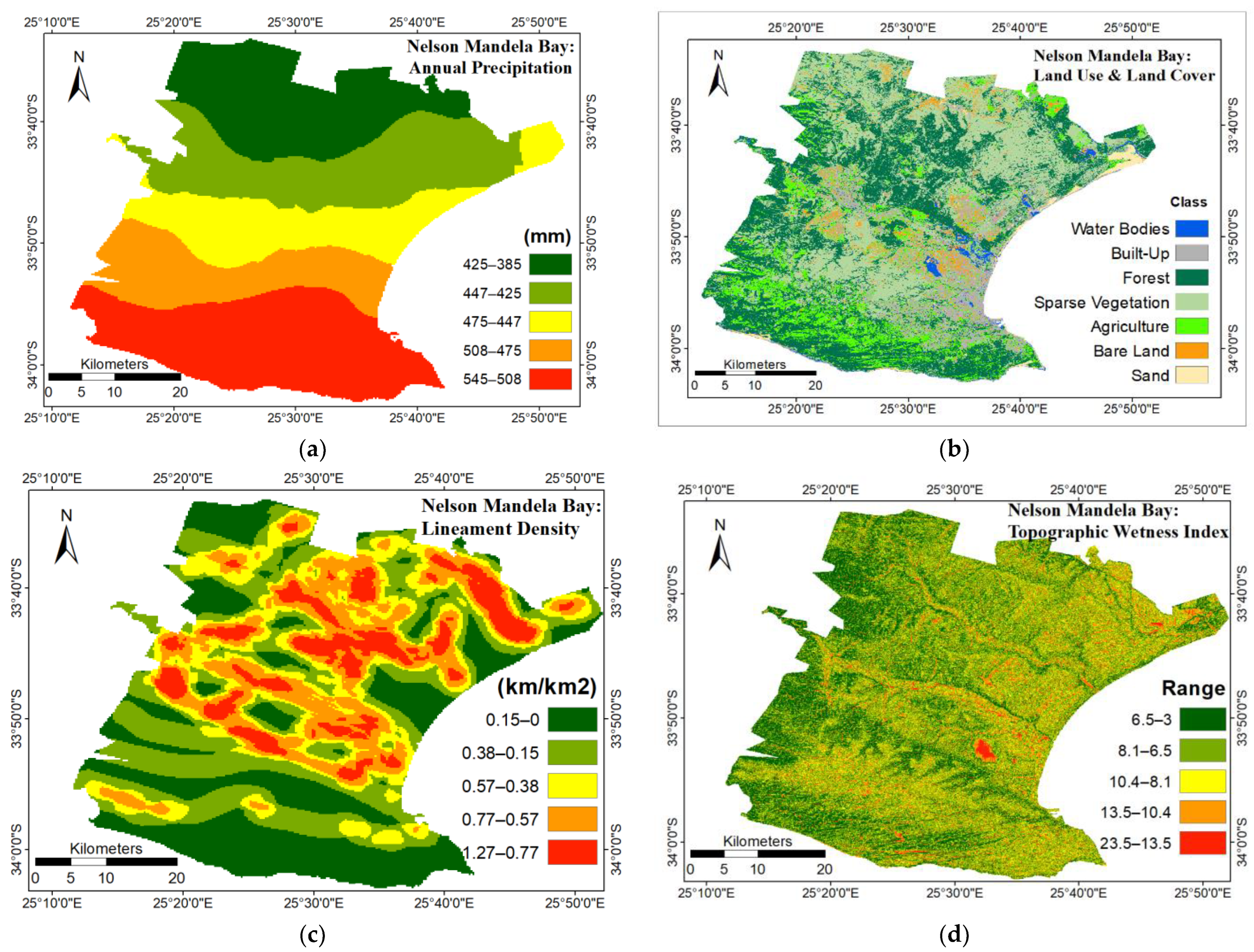
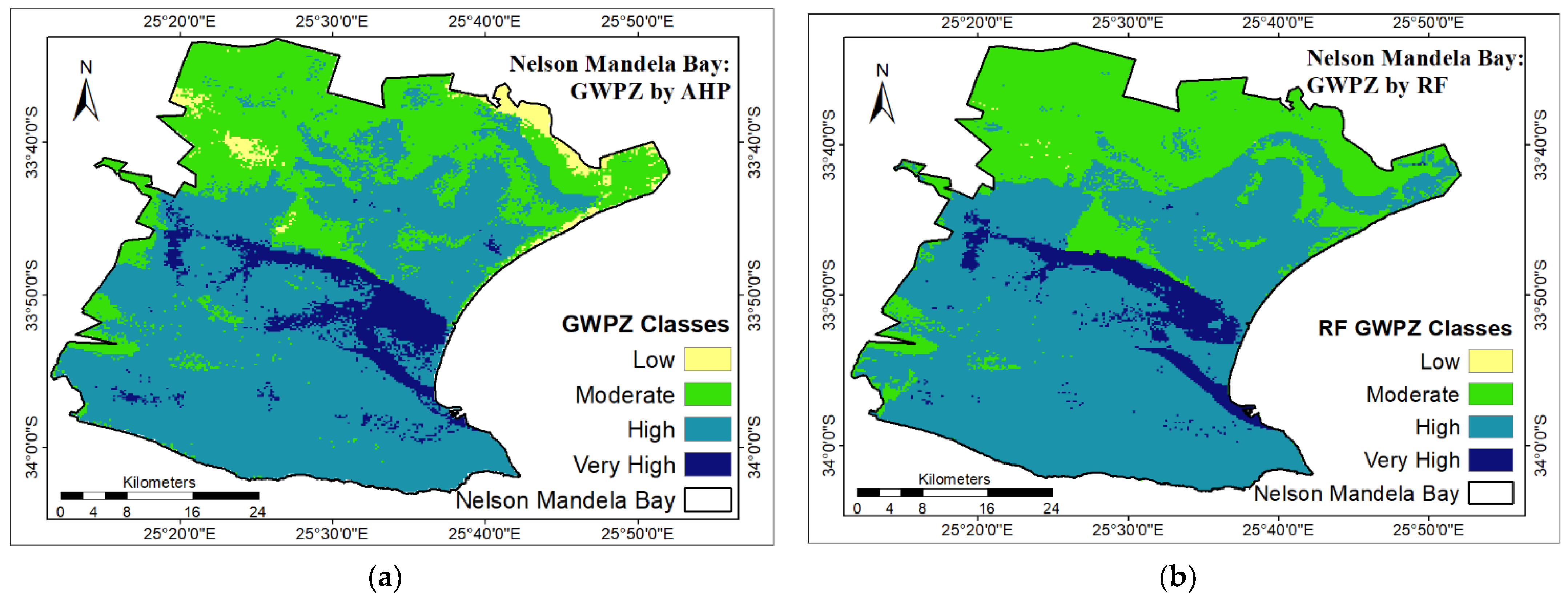
In the present study, the primary objective was to predict GWPZs using a combination of geographical information systems-based AHP and machine learning-based RF techniques. Various hydrological, topographical, remote sensing-based and lithological factors were employed as the groundwater-controlling factors, which included precipitation, land use and land cover, lineament density, topographic wetness index, drainage density, slope, lithology, and soil properties. These factors were weighted and scaled by the AHP technique and their influence on groundwater potential. A total of 1371 borehole samples were divided into 70:30 proportions for the model training (960) and model validation (411). Borehole location training data with groundwater factors were incorporated into the RF algorithm to predict GWPM output, validated by ROC, and model efficiency was compared by AUC score. The study results indicate that RF outperformed AHP, where AUC scores were 0.81 and 0.79, respectively. Both models categorized GWPZs into four distinct classes representing low, moderate, high and very high potential. The summarized outcome indicates that AHP’s GWPZ classification encompasses low (2.64%), moderate (29.88%), high (59.62%) and very high (7.86%) groundwater potential. On the other hand, RF-derived GWPZ categories were low (0.05%), moderate (31.00%), high (62.80%) and very high (6.16%) groundwater potential. Collectively, the study findings unveil that NMB is characterized by prevalent moderate to high GWPZs. Given the model’s low cost and ability to help with GWPZ prediction efficiency, groundwater potential mapping must be used to define GWPZs. The study results can be used for strategic sustainable planning of groundwater exploration, and we have addressed the GWPZs in the NMB successfully.
While the current study has successfully developed GWPM using AHP and RF models in NMB, there is a promising avenue for future research that can enhance the reliability and accuracy of groundwater predictions. Embracing ML algorithms and integrating reliable geophysical data and remote sensing information can lead to robust and accurate groundwater prediction in NMB.

Author Contributions

I.D.S. and I.A. contributed significantly to conceiving and designing this research project. This paper was a part of a master’s thesis by I.D.S. and comprehensive supervision and guidance were provided by I.A. All authors have read and agreed to the published version of the manuscript.

Funding

This research was part of a master’s degree by coursework and research funded by the South African National Space Agency (SANSA) student grant.

Data Availability Statement

The data that support the findings of this study are available on request from the corresponding author.

Acknowledgments

The meteorological data were obtained from Climate Engine, while the borehole data were sourced from the Department of Water and Sanitation Groundwater Achiever. We are deeply thankful to Muhammad Ahsan Mahboob for providing insightful review and to the anonymous reviewers for their comprehensive feedback and insightful comments. Their thoughtful feedback significantly contributed to the manuscript’s improvement.

Conflicts of Interest

The authors declare no conflict of interest.

References

  1. Eugene, R.P.; Eveth, N.A.N.; Ibrahimu, K. Ground Water Potential Zones Investigation Using Ground Magnetic Survey in South Africa. In Proceedings of the International Conference on Industrial Engineering and Operations Management, Johannesburg, South Africa, 29 October–1 November 2018; pp. 1155–1164. [Google Scholar]
  2. Ponnusamy, D.; Rajmohan, N.; Li, P.; Thirumurugan, M.; Sabarathinam, C.; Elumalai, V. Mapping of Potential Groundwater Recharge Zones: A Case Study of Maputaland Coastal Plain, South Africa. Res. Sq. 2021. preprint. [Google Scholar] [CrossRef]
  3. Bekele, T.T. Groundwater Potential Zone Delineation Using GIS and Remote Sensing Techniques in Sululta and Surrounding Watershed, Ethiopia. Int. J. Sci. Res. Eng. Dev. 2021, 4, 263–286. [Google Scholar]
  4. Abdalla, F.; Moubark, K.; Abdelkareem, M. Groundwater Potential Mapping Using GIS, Linear Weighted Combination Techniques and Geochemical Processes Identification, West of the Qena Area, Upper Egypt. J. Taibah Univ. Sci. 2020, 14, 1350–1362. [Google Scholar] [CrossRef]
  5. Moodley, T.; Seyam, M.; Abunama, T.; Bux, F. Delineation of Groundwater Potential Zones in KwaZulu-Natal, South Africa Using Remote Sensing, GIS and AHP. J. Afr. Earth Sci. 2022, 193, 104571. [Google Scholar] [CrossRef]
  6. Shandu, I.D. An Integration of Geospatial Modelling and Machine Learning Techniques for Mapping Groundwater Potential Zones in Nelson Mandela Bay, South Africa; University of Witwatersrand: Johannesburg, South Africa, 2023. [Google Scholar]
  7. Arabameri, A.; Chandra, S.; Rezaie, F.; Asadi, O.; Chowdhuri, I.; Saha, A.; Lee, S. Modeling Groundwater Potential Using Novel GIS-Based Machine-Learning Ensemble Techniques. J. Hydrol. Reg. Stud. 2021, 36, 100848. [Google Scholar] [CrossRef]
  8. Abrar, H.; Legesse Kura, A.; Esayas Dube, E.; Likisa Beyene, D. AHP Based Analysis of Groundwater Potential in the Western Escarpment of the Ethiopian Rift Valley. Geol. Ecol. Landsc. 2021, 7, 175–188. [Google Scholar] [CrossRef]
  9. MacDonald, A.M.; Bonsor, H.C.; Dochartaigh, B.É.Ó.; Taylor, R.G. Quantitative Maps of Groundwater Resources in Africa. Environ. Res. Lett. 2012, 7, 024009. [Google Scholar] [CrossRef]
  10. Hakim, W.L.; Nur, A.S.; Rezaie, F.; Panahi, M.; Lee, C.W.; Lee, S. Convolutional Neural Network and Long Short-Term Memory Algorithms for Groundwater Potential Mapping in Anseong, South Korea. J. Hydrol. Reg. Stud. 2022, 39, 100990. [Google Scholar] [CrossRef]
  11. Prasad, P.; Loveson, V.J.; Kotha, M.; Yadav, R. Application of Machine Learning Techniques in Groundwater Potential Mapping along the West Coast of India. Gisci. Remote Sens. 2020, 57, 735–752. [Google Scholar] [CrossRef]
  12. Ahirwar, R.; Malik, M.S.; Ahirwar, S.; Shukla, J.P. Groundwater Potential Zone Mapping of Hoshangabad and Budhni Industrial Area, Madhya Pradesh, India. Groundw. Sustain. Dev. 2021, 14, 100631. [Google Scholar] [CrossRef]
  13. Nampak, H.; Pradhan, B.; Manap, M.A. Application of GIS Based Data Driven Evidential Belief Function Model to Predict Groundwater Potential Zonation. J. Hydrol. 2014, 513, 283–300. [Google Scholar] [CrossRef]
  14. Fajana, A.O. Groundwater Aquifer Potential Using Electrical Resistivity Method and Porosity Calculation: A Case Study. NRIAG J. Astron. Geophys. 2020, 9, 168–175. [Google Scholar] [CrossRef]
  15. Gintamo, T.T. Ground Water Potential Evaluation Based on Integrated GIS and Remote Sensing Techniques, in Bilate River Catchment: South Rift Valley of Ethiopia. Am. Sci. Res. J. Eng. Technol. Sci. 2015, 10, 85–120. [Google Scholar]
  16. Víctor, G.E.; Marie-Louise, V.; Elisa, D.; Moussa, I.; Giaime, O.; Daira, D.; Pedro, M.S.; Francesco, H. Delineation of Groundwater Potential Zones by Means of Ensemble Tree Supervised Classification Methods in the Eastern Lake Chad Basin. Geocarto Int. 2021, 37, 8924–8951. [Google Scholar] [CrossRef]
  17. Ndhlovu, G.Z.; Woyessa, Y.E. Integrated Assessment of Groundwater Potential Using Geospatial Techniques in Southern Africa: A Case Study in the Zambezi River Basin. Water 2021, 13, 2610. [Google Scholar] [CrossRef]
  18. Shao, Z.; Huq, M.E.; Cai, B.; Altan, O.; Li, Y. Integrated Remote Sensing and GIS Approach Using Fuzzy-AHP to Delineate and Identify Groundwater Potential Zones in Semi-Arid Shanxi Province, China. Environ. Model. Softw. 2020, 134, 104868. [Google Scholar] [CrossRef]
  19. Sresto, M.A.; Siddika, S.; Haque, M.N.; Saroar, M. Application of Fuzzy Analytic Hierarchy Process and Geospatial Technology to Identify Groundwater Potential Zones in North-West Region of Bangladesh. Environ. Chall. 2021, 5, 100214. [Google Scholar] [CrossRef]
  20. Razandi, Y.; Pourghasemi, H.R.; Neisani, N.S.; Rahmati, O. Application of Analytical Hierarchy Process, Frequency Ratio, and Certainty Factor Models for Groundwater Potential Mapping Using GIS. Earth Sci. Inf. 2015, 8, 867–883. [Google Scholar] [CrossRef]
  21. Corsini, A.; Cervi, F.; Ronchetti, F. Weight of Evidence and Artificial Neural Networks for Potential Groundwater Spring Mapping: An Application to the Mt. Modino Area (Northern Apennines, Italy). Geomorphology 2009, 111, 79–87. [Google Scholar] [CrossRef]
  22. Park, S.; Kim, J. Landslide Susceptibility Mapping Based on Random Forest and Boosted Regression Tree Models, and a Comparison of Their Performance. Appl. Sci. 2019, 9, 942. [Google Scholar] [CrossRef]
  23. Arulbalaji, P.; Padmalal, D.; Sreelash, K. GIS and AHP Techniques Based Delineation of Groundwater Potential Zones: A Case Study from Southern Western Ghats, India. Sci. Rep. 2019, 9, 2082. [Google Scholar] [CrossRef] [PubMed]
  24. Mogaji, K.A.; Lim, H.S. Application of Dempster-Shafer Theory of Evidence Model to Geoelectric and Hydraulic Parameters for Groundwater Potential Zonation. NRIAG J. Astron. Geophys. 2018, 7, 134–148. [Google Scholar] [CrossRef]
  25. Owolabi, S.T. A Groundwater Potential Zone Mapping Approach for Semi-Arid Environments Using Remote Sensing (RS), Geographic Information System (GIS), and Analytical Hierarchical Process (AHP) Techniques: A Case Study of Buffalo Catchment, Eastern Cape, South. Arab. J. Geosci. 2020, 13, 1184. [Google Scholar] [CrossRef]
  26. Maskooni, E.K.; Naghibi, S.A.; Hashemi, H.; Berndtsson, R. Application of Advanced Machine Learning Algorithms to Assess Groundwater Potential Using Remote Sensing-Derived Data. Remote Sens. 2020, 12, 2742. [Google Scholar] [CrossRef]
  27. Hasanuzzaman, M.; Mandal, M.H.; Hasnine, M.; Shit, P.K. Groundwater Potential Mapping Using Multi-Criteria Decision, Bivariate Statistic and Machine Learning Algorithms: Evidence from Chota Nagpur Plateau, India. Appl. Water Sci. 2022, 12, 58. [Google Scholar] [CrossRef]
  28. Ghanim, A.A.J.; Shaf, A.; Ali, T.; Zafar, M.; Al-areeq, A.M.; Alyami, S.H.; Irfan, M.; Rahman, S. An Improved Flood Susceptibility Assessment in Jeddah, Saudi Arabia, Using Advanced Machine Learning Techniques. Water 2023, 15, 2511. [Google Scholar] [CrossRef]
  29. Lee, S.; Hyun, Y.; Lee, S.; Lee, M.J. Groundwater Potential Mapping Using Remote Sensing and GIS-Based Machine Learning Techniques. Remote Sens. 2020, 12, 1200. [Google Scholar] [CrossRef]
  30. Mdegela, L.; Municio, E.; De Bock, Y.; Luhanga, E.; Leo, J.; Mannens, E. Extreme Rainfall Event Classification Using Machine Learning for Kikuletwa River Floods. Water 2023, 15, 1021. [Google Scholar] [CrossRef]
  31. Razavi-Termeh, S.V.; Sadeghi-Niaraki, A.; Choi, S.M. Groundwater Potential Mapping Using an Integrated Ensemble of Three Bivariate Statistical Models with Random Forest and Logistic Model Tree Models. Water 2019, 11, 1596. [Google Scholar] [CrossRef]
  32. Sameen, M.I.; Pradhan, B.; Lee, S. Self-Learning Random Forests Model for Mapping Groundwater Yield in Data-Scarce Areas. Nat. Resour. Res. 2019, 28, 757–775. [Google Scholar] [CrossRef]
  33. Panahi, M.; Sadhasivam, N.; Pourghasemi, H.R.; Rezaie, F.; Lee, S. Spatial Prediction of Groundwater Potential Mapping Based on Convolutional Neural Network (CNN) and Support Vector Regression (SVR). J. Hydrol. 2020, 588, 125033. [Google Scholar] [CrossRef]
  34. Kim, J.C.; Jung, H.S.; Lee, S. Spatial Mapping of the Groundwater Potential of the Geum River Basin Using Ensemble Models Based on Remote Sensing Images. Remote Sens. 2019, 11, 2285. [Google Scholar] [CrossRef]
  35. Naghibi, S.A.; Pourghasemi, H.R.; Dixon, B. GIS-Based Groundwater Potential Mapping Using Boosted Regression Tree, Classification and Regression Tree, and Random Forest Machine Learning Models in Iran. Environ. Monit. Assess. 2016, 188, 44. [Google Scholar] [CrossRef] [PubMed]
  36. Klages, N. Nelson Mandela Bay Municipality State of the Environment Report; Nelson Mandela Bay Metropolitan Municipality: Nelson Mandela Bay, South Africa, 2011; 152p.
  37. Baron, J. Eastern Cape Groundwater Plan; Department of Water Affairs: Port Elizabeth, South Africa, 2010; pp. 1–41.
  38. Patidar, R.; Pingale, S.M.; Khare, D. An Integration of Geospatial and Machine Learning Techniques for Mapping Groundwater Potential: A Case Study of the Shipra River Basin, India. Arab. J. Geosci. 2021, 14, 1645. [Google Scholar] [CrossRef]
  39. Hanchane, M.; Kessabi, R.; Krakauer, N.Y.; Sadiki, A.; El Kassioui, J.; Aboubi, I. Performance Evaluation of TerraClimate Monthly Rainfall Data after Bias Correction in the Fes-Meknes Region (Morocco). Climate 2023, 11, 120. [Google Scholar] [CrossRef]
  40. Ghosh, P.K.; Bandyopadhyay, S.; Jana, N.C. Mapping of Groundwater Potential Zones in Hard Rock Terrain Using Geoinformatics: A Case of Kumari Watershed in Western Part of West Bengal. Model. Earth Syst. Environ. 2015, 2, 1. [Google Scholar] [CrossRef]
  41. Díaz-Alcaide, S.; Martínez-Santos, P. Review: Advances in Groundwater Potential Mapping. Hydrogeol. J. 2019, 27, 2307–2324. [Google Scholar] [CrossRef]
  42. Wiesmeier, M.; Barthold, F.; Blank, B.; Kögel-Knabner, I. Digital Mapping of Soil Organic Matter Stocks Using Random Forest Modeling in a Semi-Arid Steppe Ecosystem. Plant Soil 2011, 340, 7–24. [Google Scholar] [CrossRef]
  43. Melese, T.; Belay, T. Groundwater Potential Zone Mapping Using Analytical Hierarchy Process and GIS in Muga Watershed, Abay Basin, Ethiopia. Glob. Chall. 2022, 6, 2100068. [Google Scholar] [CrossRef]
  44. Tamiru, H.; Wagari, M. Comparison of ANN Model and GIS Tools for Delineation of Groundwater Potential Zones, Fincha Catchment, Abay Basin, Ethiopia. Geocarto Int. 2021, 37, 6736–6754. [Google Scholar] [CrossRef]
  45. Rahmati, O.; Reza, H.; Melesse, A.M. Catena Application of GIS-Based Data Driven Random Forest and Maximum Entropy Models for Groundwater Potential Mapping: A Case Study at Mehran Region, Iran. Catena 2016, 137, 360–372. [Google Scholar] [CrossRef]
  46. Breiman, L. Random Forests. Random For. 2001, 45, 5–32. [Google Scholar] [CrossRef]
  47. Kumar, A.; Pramanik, M.; Chaudhary, S.; Negi, M.S.; Szabo, S. Geospatial Multi-Criteria Evaluation to Identify Groundwater Potential in a Himalayan District, Rudraprayag, India; Springer: Dordrecht, The Netherlands, 2022. [Google Scholar]
Figure 1. Nelson Mandela Bay district spatial location.
Water 15 03447 g001
Figure 2. Comprehensive flowchart outlining the methodology for modelling of groundwater potential zones (GWPZs) [5,31,38].
Water 15 03447 g002
Figure 3. Thematic input for groundwater conditional factors: (a) precipitation; (b) LULC; (c) LD; (d) TWI; (e) DD; (f) slope; (g) lithology; and (h) soil.
Water 15 03447 g003aWater 15 03447 g003b
Figure 4. Groundwater potential zone map of Nelson Mandela Bay: (a) geospatial modelling based on AHP, and (b) machine learning-based RF.
Water 15 03447 g004
Figure 5. AUC and ROC for GWPZs by RF and AHP models in Nelson Mandela Bay.
Water 15 03447 g005
Table 1. Groundwater-controlling factors’ data sources.
ParameterData SourceSensor and Spatial Resolution
BoreholesDepartment of Water and SanitationVector Layer
Drainage Density USGS Earth Explore Shuttle Radar Topographic Mission (SRTM); 30 m (1 arc–s)
PrecipitationTerraClimate; Climate Data Engine TerraClimate; ~4 km (1/24th degree) grid
LULCSentinel Hub; Google Earth Engine (GEE) ProcessingSentinel 2; [B2–B4, B8] 10 m & [B1, B5–B7, B8A, B9] 60 m
Slope USGS Earth Explore SRTM; ~30 m (1 arc–s)
TWIUSGS Earth Explore SRTM; ~30 m (1 arc–s)
SoilInternational Soil Reference and Information Centre (ISRIC)—Soil Data HubVector Layer
LithologyISRIC Soil Data HubVector Layer
Lineament Density Council of GeoscienceVector Layer
Table 2. Saaty’s scale of importance measure for evaluating pairwise comparison matrix of parameters.
ParameterData Source
1Equal importance
2Weak
3Moderate importance
4Moderate plus
5Strong plus
6Strong importance
7Very strong importance
8Very-very strong importance
9Extreme importance
Table 3. Pairwise comparison matrix for the thematic layers used in the delineation of GWPZs based on AHP.
Thematic LayerPrecipitationLULCLDTWIDDSlopeLithologySoil
Precipitation15254525
LULC1/511/511/311/31
LD1/5214131/33
TWI1/511/411/51/31/41/3
DD1/431/35111/31
Slope1/411/331/311/41
Lithology15343416
Soil1/511/33111/61
Table 4. Standardized pairwise comparison matrix for the thematic layers in groundwater potential zone delineation using AHP.
Thematic LayerPrecipitationLULCLDTWIDDSlopeLithologySoilWeight
Precipitation0.300.260.270.190.370.310.430.2730.0%
LULC0.060.050.030.040.030.060.070.055.0%
LD0.060.110.130.150.090.180.070.1612.1%
TWI0.060.050.030.040.020.020.050.023.7%
DD0.080.160.040.190.090.060.070.059.4%
Slope0.080.050.040.120.030.060.050.056.1%
Lithology0.300.260.400.150.280.240.210.3327.3%
Soil0.060.050.040.120.090.060.040.056.5%
Table 5. Random consistency matrix and ratio for the correspondence number of groundwater-controlling parameters used for GWPM.
N12345678910
RI000.580.91.121.241.321.411.451.49
Note: RI is Saaty’s random index or random consistency values for the matrix [5].
Table 6. Groundwater-controlling parameters thematic layer relative weighting and ranking based on AHP technique [5,6,17,23].
Thematic LayerClassesRankAssigned RankWeight
Precipitation (mm)384–425 3Very low30.0%
425–447 4Low
447–475 5Moderate
475–508 6High
508–546 7Very high
LULCAgriculture land6High5.0%
Bare land1Very low
Forest5Moderate
Sand6High
Sparse vegetation2Low
Built-up1Very low
Water bodies7Very high
LD (km/km²)0.00–0.152Very low12.1%
0.15–0.383Low
0.38–0.574Moderate
0.57–0.775High
0.77–1.276Very high
TWI03–6.51Very low3.7%
6.5–8.13Low
8.1–10.44Moderate
10.4–13.55High
13.5–23.56Very high
DD (km/km²)0.0–0.56Very high9.4%
0.5–0.85High
0.8–1.14Moderate
1.1–1.43Low
1.4–1.91Very low
Slope (°)0–36Very high6.1%
3–75High
7–134Moderate
13–223Low
>222Very low
LithologyLimestone4Moderate27.3%
Sandstone3Low
Seychelles/granite1Very low
Shale5High
Siltstone6Very high
SoilLoamy sand7High6.5%
Sand9Very high
Sandy clay4Very low
Sandy clay loam5Low
Sandy loam6Moderate
Table 7. Spatial locations of borehole and potential of groundwater zones delineated by RF and AHP models in Nelson Mandela Bay.
CodeClassAHP-GWPZs RF-GWPZs
Boreholes Boreholes
1Low31
2Moderate205198
3High10001008
4Very High163164
Disclaimer/Publisher’s Note: The statements, opinions and data contained in all publications are solely those of the individual author(s) and contributor(s) and not of MDPI and/or the editor(s). MDPI and/or the editor(s) disclaim responsibility for any injury to people or property resulting from any ideas, methods, instructions or products referred to in the content.

