Abstract
The Xiaolangdi reservoir has a storage capacity of more than 10 billion cubic meters, and the dam has significant seasonal deformation. Predicting the deformation of the dam during different periods is important for the safe operation of the dam. In this study, a long short-term memory (LSTM) model based on interferometric synthetic aperture radar (InSAR) deformation data is introduced to predict dam deformation. First, a time series deformation model of the Xiaolangdi Dam for 2017–2023 was established using Sentinel-1A data with small baseline subset InSAR (SBAS-InSAR), and a cumulative deformation accuracy of 95% was compared with the on-site measurement data at the typical point P. The correlation between reservoir level and dam deformation was found to be 0.81. Then, a model of reservoir level and dam deformation predicted by neural LSTM was established. The overall deformation error of the dam was predicted to be within 10 percent. Finally, we used the optimized reservoir level to simulate the deformation at the measured point P of the dam, which was reduced by about 36% compared to the real deformation. The results showed that the combination of InSAR and LSTM could predict dam failure and prevent potential failure risks by adjusting the reservoir levels.
1. Introduction
Rockfill dams are large hydraulic structures composed of various rock materials equipped with impermeable core walls made of special materials. Dams play important roles in terms of water storage, flood control, sand drainage, and power generation. They have a great influence on the development of industry and agriculture and the local geological environment [1,2].
During the construction of a rockfill dam, different materials are used in different embankment zones; the same embankment zone may be constructed differently in the field, leading to inevitable differences in deformation in different areas of the dam [3]. After the dam is completed and commissioned, the reservoir begins to store water and adjusts its level according to certain rules. The dam body also undergoes seasonal deformation as the hydrostatic pressure on the dam changes with the rainfall and reservoir levels [4].
Rockfill dams have more complex deformation characteristics than conventional structures or concrete dams. To assess the overall structural health in a timely manner, the periodic deformation monitoring of dams is essential. It can be used to predict how a dam will deform over a period of time in the future to determine if any safety hazards exist and to take appropriate actions to prevent the main body of the dam from crumbling or collapsing [5].
Most traditional dam deformation monitoring methods use geodetic techniques, such as using level and total station measurements for observations [6]. In addition, more sophisticated global satellite positioning techniques can be employed [7]. Sensors such as embedded flexible pipes can also be installed inside dams for monitoring [8]. Although these methods are widely used, they are labor-intensive and expensive. In addition, these methods can only reflect the deformation of monitoring points or lines. However, they do not accurately reflect the overall deformation of a dam. Some scholars have used numerical simulations to reconstruct the deformation characteristics of an entire dam using similar methods, provided that the design and construction parameters of each part of the dam are available, and the overall deformation is calculated via computer simulations [9,10]. Currently, many rockfill dams were built and put into operation worldwide so early that some of the dam parameters are missing, and this method cannot be used.
Interferometric synthetic aperture radar (InSAR) can acquire information on the deformation of the Earth’s surface on a millimeter scale over time [11]. It has been widely used to map deformations caused by geological events, such as landslides, earthquakes, and volcanic eruptions [12,13,14,15]. It has also achieved good results in monitoring the effects of human activities such as mining, groundwater extraction, road subsidence, and urban development [16,17,18,19,20,21,22,23,24]. In addition, large regional surface studies, such as polar permafrost and glacier monitoring, have great potential [25,26,27].
With respect to the monitoring of dam deformation using InSAR, Zhou et al. [28,29] showed that the overall deformation of the Shuibuya Dam obtained using the multiple-temporal InSAR (MT-InSAR) technique is in agreement with the results of in situ geodetic measurements. On this basis, the numerical model of dam deformation using finite element analysis can be complemented by surface deformation monitored via InSAR. Ruiz-Armenteros et al. [30] used MT-InSAR to study a dam in southern Spain and observed significant vertical settlement in the main body of the dam, with deformations mainly distributed in the center of the dam and part of the slope adjacent to the dam. Biondi et al. [31] studied the deformation characteristics of the Mosul Dam using the PS-InSAR technique and showed significant settlement at the center of the dam and opposite deformation trends at the two ends of the dam. A crack was found in the dam that seriously threatened its safe operation. Xiao et al. [32] combined ICEsat-2, Sentinel-1, and Sentinel-2 satellite data and used the small baseline subset InSAR (SBAS-InSAR) technique to investigate the failure of the Sardoba Dam in 2020. The dam failure section showed abnormal settlement, and it was hypothesized that seepage may have occurred inside the dam, resulting in changes in the pressure-bearing capacity and structural stability of the dam, thereby causing the accident. Bayik, Abdikan, and Arıkan [33] monitored the Atatürk Dam in Turkey using multiple images from three satellites, ERS, ENVISAT, and Sentinel-1A, in different orbits, and they found that the dam was still settling 28 years after its construction. However, the deformation characteristics of the dam were different in different periods and showed that the water storage level and the dam deformation were not always correlated.
Long short-term memory (LSTM) is one of the most influential methods in the field of deep learning [34,35,36,37,38], and many researchers have used LSTM models to explore the potential information of data in investigations such as surface observations. Jean et al. [39] used an LSTM model to assess seismic vulnerability across India and prioritize areas in need of protective measures. Li et al. [40] achieved real-time monitoring and prediction of landslide displacement using a deep learning framework based on LSTM to study landslides in the Three Gorges area of China. Chen et al. [41] used the LSTM model based on sliding window data to build a model for predicting future precipitation with precipitation data of up to 40 years in some regions of Turkey as the dependent variable and analyzed the lag period of the precipitation time series by adjusting the model’s hyperparameter. Radman, Akhoondzadeh, and Hosseiny [42] used the InSAR technique to obtain surface deposition data near Lake Urmia in Iran and developed a predictive LSTM model combining environmental parameters such as groundwater content to investigate the driving factors affecting surface deposition. The LSTM model proved to be excellent for the time series data. We used longer-period InSAR deformation data and combined them with daily water storage level data to better utilize the data mining capability of LSTM.
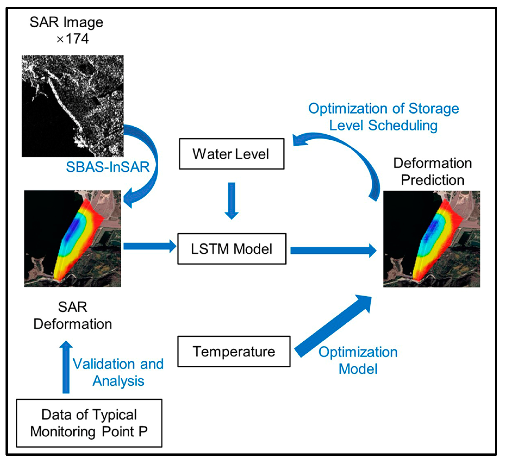
The overall workflow diagram of this study is shown in Figure 1, and the main work can be divided into three parts:

Figure 1.
The overall workflow diagram of this study.
- (1)
- Obtain the spatial and temporal evolution characteristics of dam surface deformation by constructing a time series model of the Xiaolangdi Dam using SBAS-InSAR.
- (2)
- Analyze the deformation law of the InSAR model and propose an LSTM network model using water storage level data to predict the surface deformation of the dam.
- (3)
- Optimize the prediction model and propose a reservoir level scheduling scheme and finally verify the feasibility of the scheme using the InSAR-LSTM deformation prediction model.
2. Materials
2.1. Study Area
The Xiaolangdi Dam was constructed in 2001 and is located 40 km north of Luoyang City, Henan Province, China, on the main stream of the Yellow River, as shown in Figure 2. The dam is a comprehensive large-scale water conservancy project that integrates siltation reduction, flood control, water supply control, irrigation, and power generation. The dam is a key project in the management and development of the Yellow River, controlling a total basin area of 694,000 km2, accounting for 92.3% of the Yellow River.
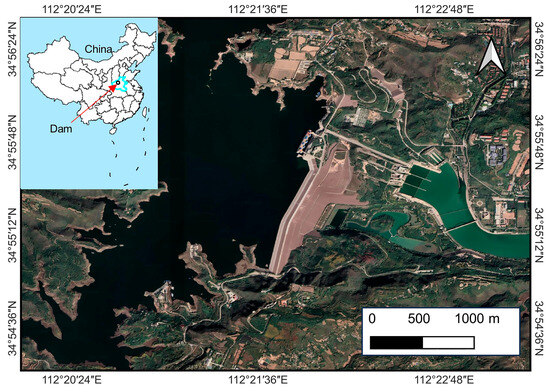
Figure 2.
Diagram of the location of Xiaolangdi Dam.
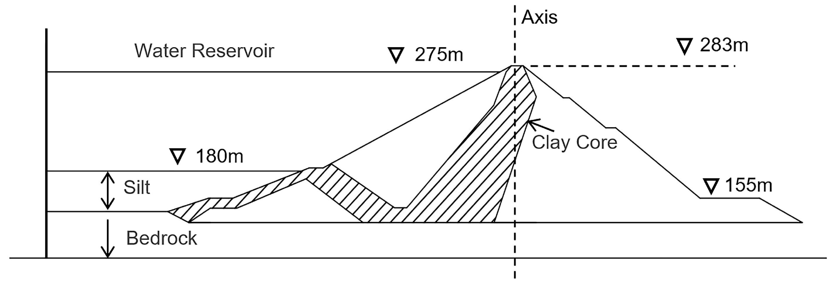
Figure 3 shows the structure of the dam. The inside of the dam is a clay-inclined core wall that prevents water seepage, whereas the outside is composed of rock and clay. With a storage capacity of 12.65 billion m3, the highest elevation of the dam is 283 m. The normal storage level is 275 m, the heads above and below the dam are approximately 100 m, and the highest historical water storage level was 273.35 m.
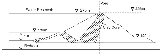
Figure 3.
Schematic diagram of the main structure of Xiaolangdi Dam.
2.2. Dataset
In this study, the radar image data used were from the Sentinel-1 satellite launched by the Copernicus program of the European Space Agency, using the data type single look complex (SLC) and the polarization method of vertical send and vertical receive (VV). This satellite is equipped with a C-band (5.6 cm wavelength) SAR sensor, the satellite revisit period is 12 days, and the acquisition interval for a few phases of images is 24 days. The imaging mode was interferometric wide-width (IW), with each image having a width of 250 km and resolution of 5 × 20 m. A total of 174 images acquired in the Earth’s ascending orbit were used in this study, and the experimental area and coverage of the images are shown in Figure 4a.
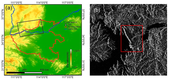
Figure 4.
(a) The schematic diagram of the location of the Sentinel-1 image. The black box in the figure is the coverage area before the image is cropped. (b) The SAR image of the dam and the red box is the range of the main body of the dam.
3. Methods
3.1. InSAR Deformation Model
The InSAR technique uses the phase difference between two satellite passes to obtain a ground digital elevation model [43]. The differential InSAR (D-InSAR) technique introduces an external DEM based on two images to obtain surface deformation information [44]. The application of D-InSAR for regional deformation monitoring is often affected by orbital parameter errors, topographic data errors, phase noise caused by interference loss correlations, phase decoupling errors, and atmospheric delays. To solve this problem, Ferretti proposed the PS-InSAR technique, which eventually formed the technical theoretical system of MT-InSAR [45,46,47,48,49,50]. Its classical methodological theory, SBAS-InSAR, can perform phase analysis on coherent targets to obtain time series deformations. Its powerful ability to model time series deformations has been demonstrated in many studies [51,52,53].
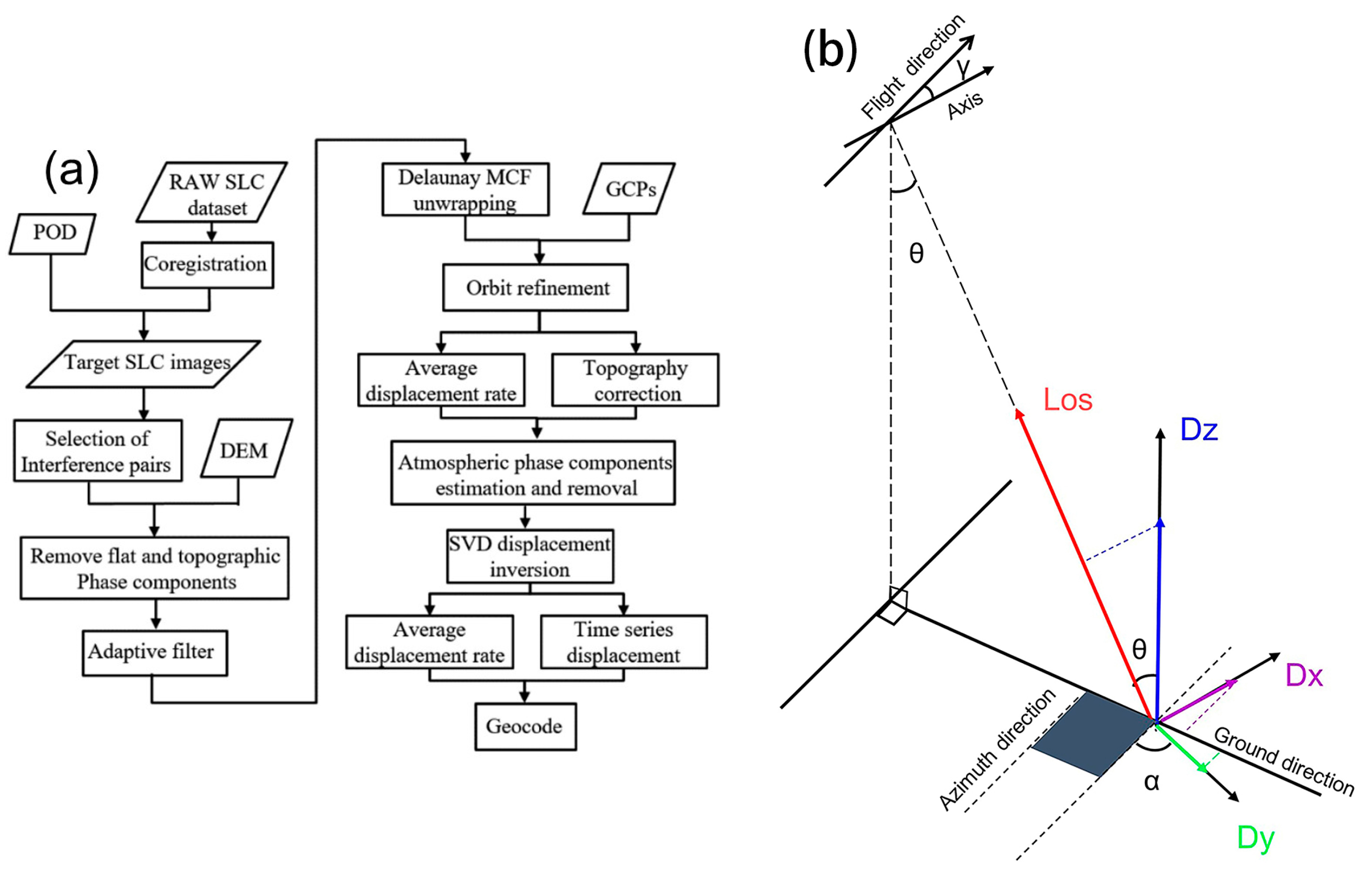
In this study, we used SBAS-InSAR to process Sentinel-1 data and build a time series model of dam deformation, as shown in Figure 5a. After acquiring the raw image data, all the images were corrected using the precision orbit data provided by the ESA. The data were assembled into differential interferometric image pairs according to a time–space baseline of 90 days and 2% of the maximum spatial baseline of all images. The topographic phases were removed using SRTM DEM data at a 90 m resolution which were acquired by the US Space Shuttle. The data were filtered using Goldstein’s algorithm [54]. The phase was deconvolved using a minimum-cost flow algorithm [52]. External control points were introduced for trajectory refinement, and the mean displacement rate of the observation points was obtained for terrain correction. The atmospheric phase was estimated and removed in the next step, and the deformation was inverted using the singular value decomposition method to generate a deformation model of the mean displacement rate and time series and finally geocoded to transfer the deformation from the radar coordinate system to the geographic coordinate system.
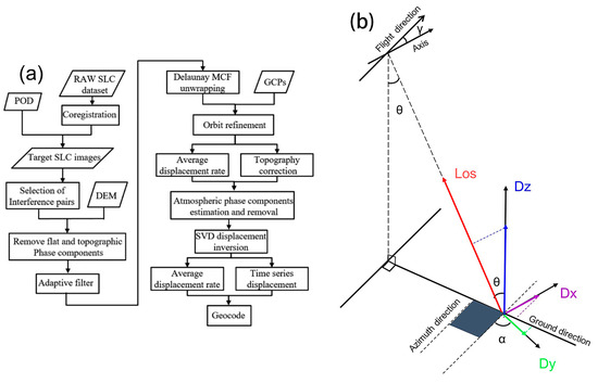
Figure 5.
(a) SBAS-InSAR data processing. (b) Projection of the on–site measurement data of the dam deformation at typical point P.
3.2. Validation of InSAR Deformation Model Reliability
Synthetic-aperture radar acquires images through side-view imaging, which allows us to obtain the deformation of the observation point in the line of sight (Los) of the satellite. This result expresses the variation in the distance between the observation point and the satellite platform.
The deformation of the observation point in the image is the 3D deformation of the ground point projected onto the image coordinates [55]. Ground truth data can be used to verify the reliability of the InSAR deformation model because the deformation of the ground observation point is usually a joint effect of deformation in multiple directions.
In general, the coordinate system used in geodetic techniques is a geographic coordinate system consisting of north, south, east, and west vertical directions. In this study, we used the measured deformation data of the Xiaolangdi Dam at the on-site point P, and the coordinate system of the data was the local coordinate system of the dam, including the three-dimensional deformation along the dam axis, perpendicular to the dam axis, and in the vertical direction.
We projected the three components of the dam axis, perpendicular to the dam axis, and vertical direction to the satellite’s line of sight according to Equation (1), as shown in Figure 5b. Dx represents the dam axis direction component, which is positive to the left bank of the dam; Dy is perpendicular to the dam axis direction component, which is positive downstream of the dam; and Dz represents the vertical direction component, which is positive in the upward direction. The angle between the flight direction of the satellite platform and the dam axis is γ. θ is the radar incidence angle, which is the angle between the radar line of sight and the vertical direction. α is the magnitude of the angle of the Dx positive direction clockwise to the satellite flight direction (analogous to the satellite heading angle in the geographic coordinate system).
3.3. InSAR Deformation Prediction Model
3.3.1. LSTM Neural Network
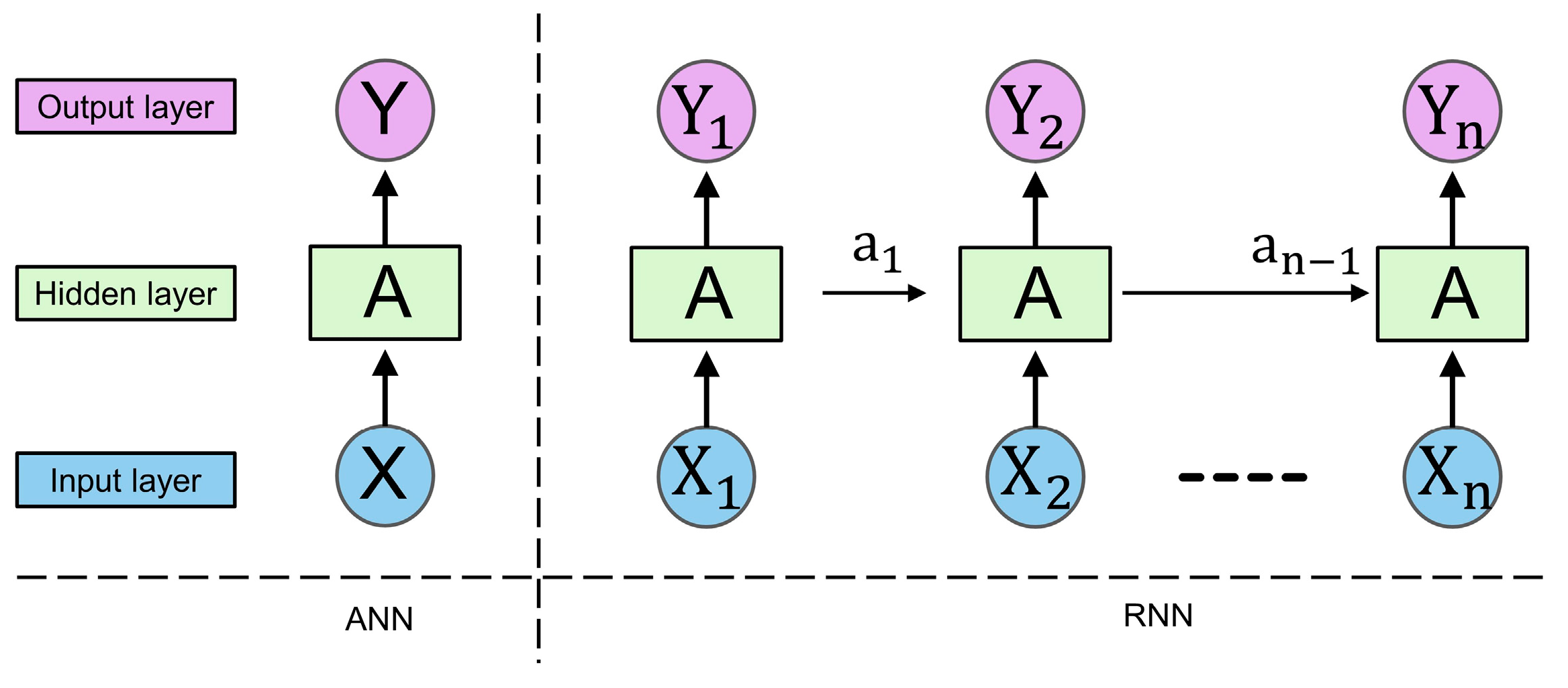
Deep learning is revolutionizing artificial intelligence around the world [56,57]. An artificial neural network (ANN) is the foundation of deep learning. The artificial neural network model consists of fully connected layers, which can be classified into input, hidden, and output layers. The activation function is at the core of a neural network. The input data are controlled using the activation function. Sigmoid, tanh, and ReLU are the most commonly used activation functions. In this model, the layers are connected by weights. The neural network learns to determine the weights between layers through training. In traditional neural networks, information is transmitted from the input to the output layer. This process can be considered independent. This implies that the output depends only on the current inputs. However, in many realistic tasks, the network output depends not only on the current input but also on its past output.
A recurrent neural network (RNN) takes sequence data as input, iterates in the direction of sequence evolution, and connects all nodes (recurrent units) in a chain fashion. The hidden layer contains a state vector that stores the historical information of all past elements and weights of the entire network. Compared with artificial neural networks, recurrent neural networks can jointly determine the output of the current moment and are more suitable for time series problems, as shown in Figure 6.

Figure 6.
The schematic diagram of the model structure of ANN and RNN.
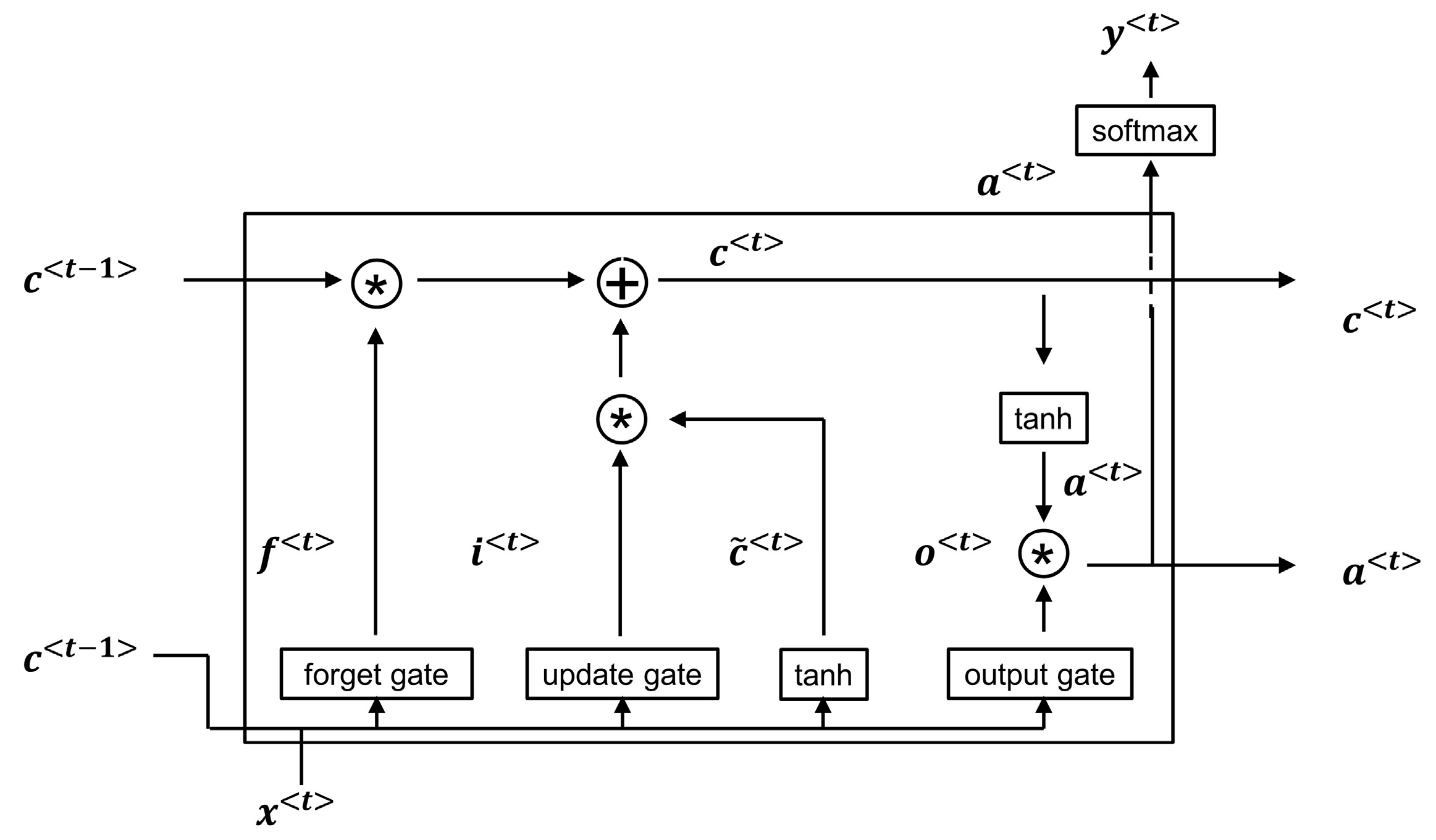
Although recurrent neural networks are used to process time series data, in practice, storing such information for a long time is difficult. The gradient explosion problem occurs in long-term dependency problems. In response, LSTM networks incorporate a special control unit (memory cell) into the recurrent neural network, as shown in Figure 7.
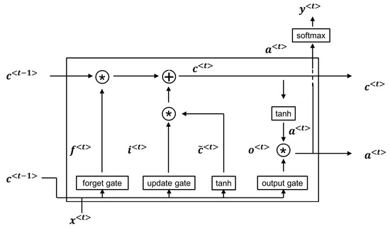
Figure 7.
The computation process of the LSTM memory unit, the asterisk in the figure indicates the multiplication operation.
The specific computational process is shown in Equations (2a)–(2f), where the memory cell consists of a control gate, update gate, and forget gate. After the data at time t, the hidden layer state vector and the cell state parameter are inputted into the LSTM cell, the candidate value for the cell state parameter update is first generated by the tanh activation function, and then and are inputted into the update cell; the update weight , the forget weight , and the output weight are calculated using the Sigmoid activation function, and the of the next LSTM cell is determined according to and , while the of the next cell is determined using the output weight . Thus, the LSTM cells are calculated.
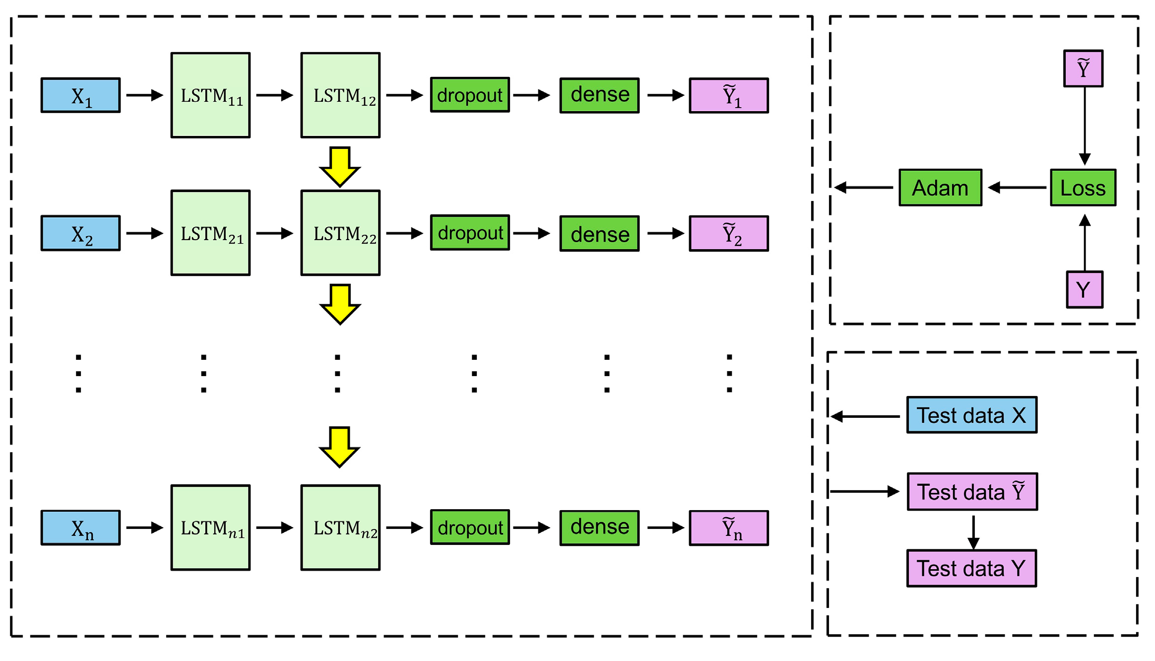
3.3.2. Construction of the Prediction Model
The structure of the LSTM model used in this study is shown in Figure 8 and was implemented using the TensorFlow and sklearn modules from the Python community. Two LSTM layers were added to the model, each with a size of 50. To prevent model overfitting, a dropout layer was used to discard random nodes in the network at a scale of 0.2. Finally, the final output was transformed into a one-dimensional vector using a fully connected layer.
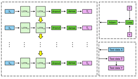
Figure 8.
The implementation process architecture of the LSTM model used in this study.
The gradient descent optimization of the loss function was performed using the Adam optimization algorithm, and the mean square error was used to evaluate the accuracy of the model. To train the model, the original data were divided into training and prediction sets, and the k-fold cross-validation method was used for the training set, where k was set to 2. In the training process, the training set was divided into two parts: one part was taken as the validation set, and the other part was taken as the training set. The GridSearchCV function was used to search for the best hyperparameters of the model and obtain the best-weight model. Finally, the test data were fed into the trained model, and the prediction results were output and validated against actual data.
4. Results and Analysis
4.1. InSAR Deformation Results and Validation
In this study, a time series model of dam deformation was established using Sentinel-1 data from March 2017 to February 2023, and the cumulative deformation of the dam body was obtained, as shown in Figure 9. In the early stages of deformation, the dam tended to be close to the satellite, with a maximum deformation value of 5 mm. In the middle stage of deformation, the center of the dam tended to be far from the satellite, whereas the left and right sides and the bottom of the dam maintained a small tendency to be close to the satellite. In the later stages of deformation, the dam as a whole tended to move away from the satellite, and there were significant differences in the deformation values in different areas, with the largest deformation value of −155 mm occurring in the middle of the top of the dam near the upstream side.
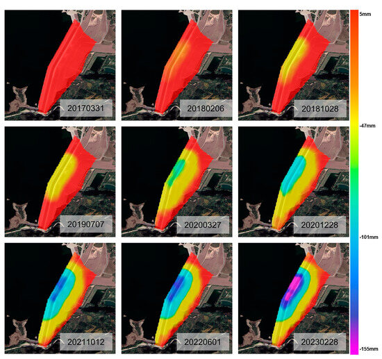
Figure 9.
The time–series variation in the cumulative deformation of Xiaolangdi Dam from March 2017 to February 2023.
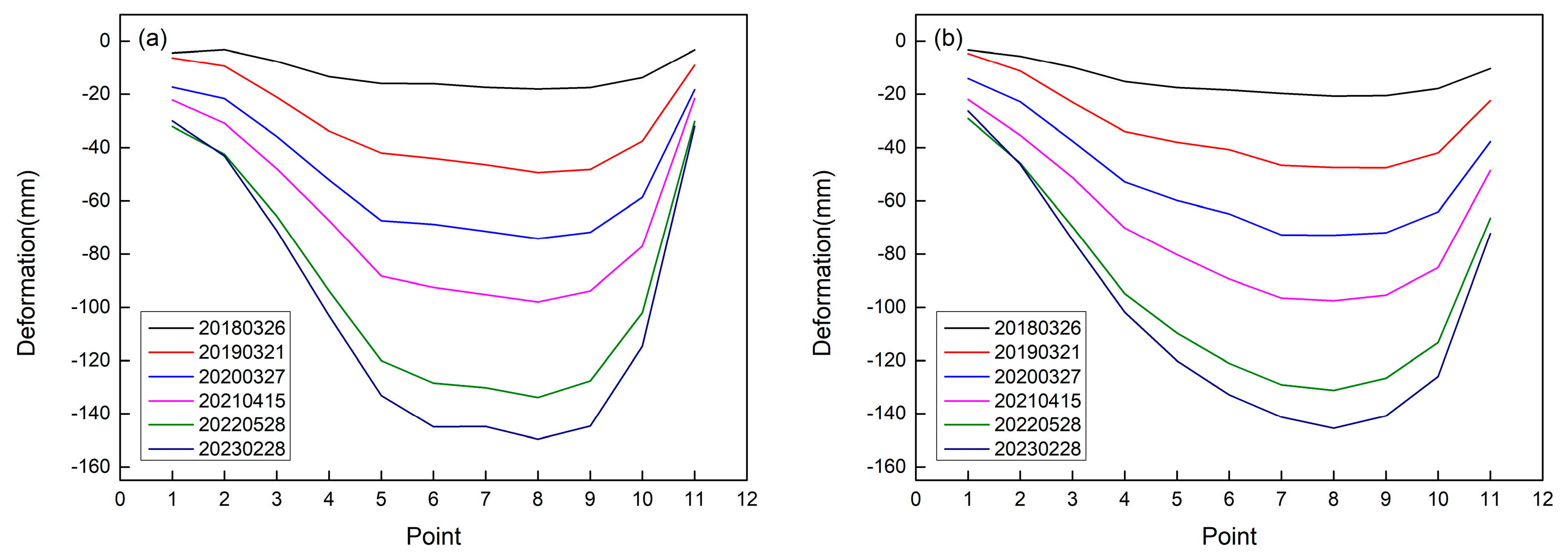
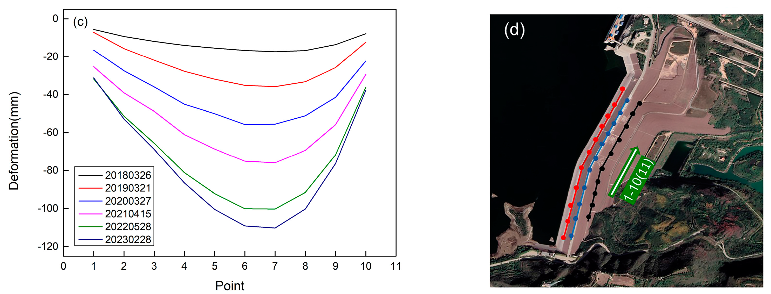
We plotted the cumulative deformation data at different times for points on the upstream slope, top, and downstream slope of the dam on lines, as shown in Figure 10. All three lines tended to have smaller deformation values on both sides, and the central part near the left side had the largest settlement value. The deformation value of the exposed water part of the upstream slope of the dam was slightly larger than that of the top of the dam, and the accumulated deformation values of the downstream slope were significantly different from those of the upstream slope and top of the dam.
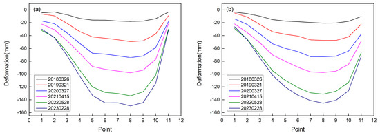

Figure 10.
(a–c) Cumulative sink value line segments of the upstream slope of the dam, the top of the dam, and on the downstream slope line, which correspond to the points on the red, blue and black lines of (d) respectively. (d) Schematic diagram of the location of the three lines; the serial numbers of the points become larger in the direction of the arrow.
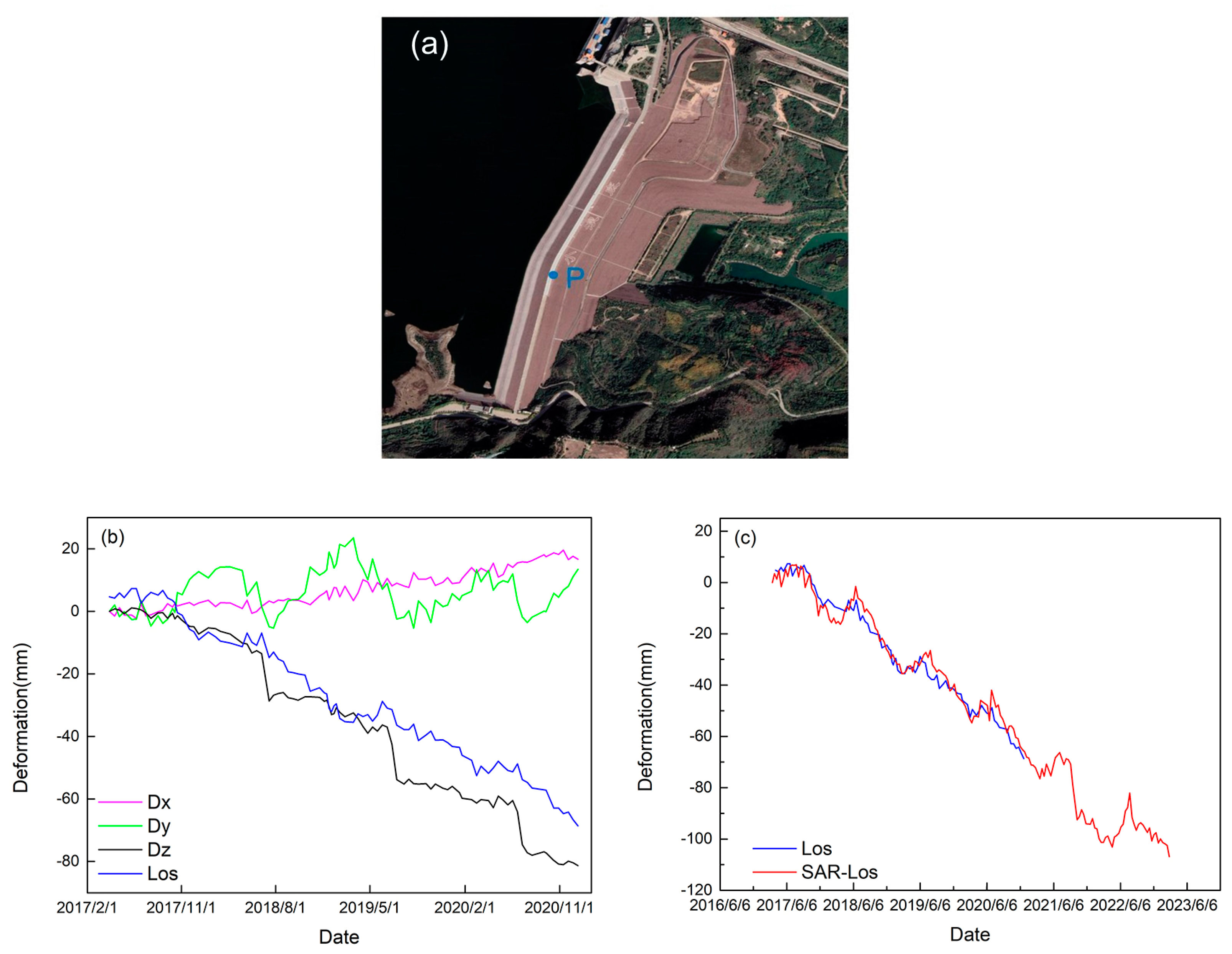
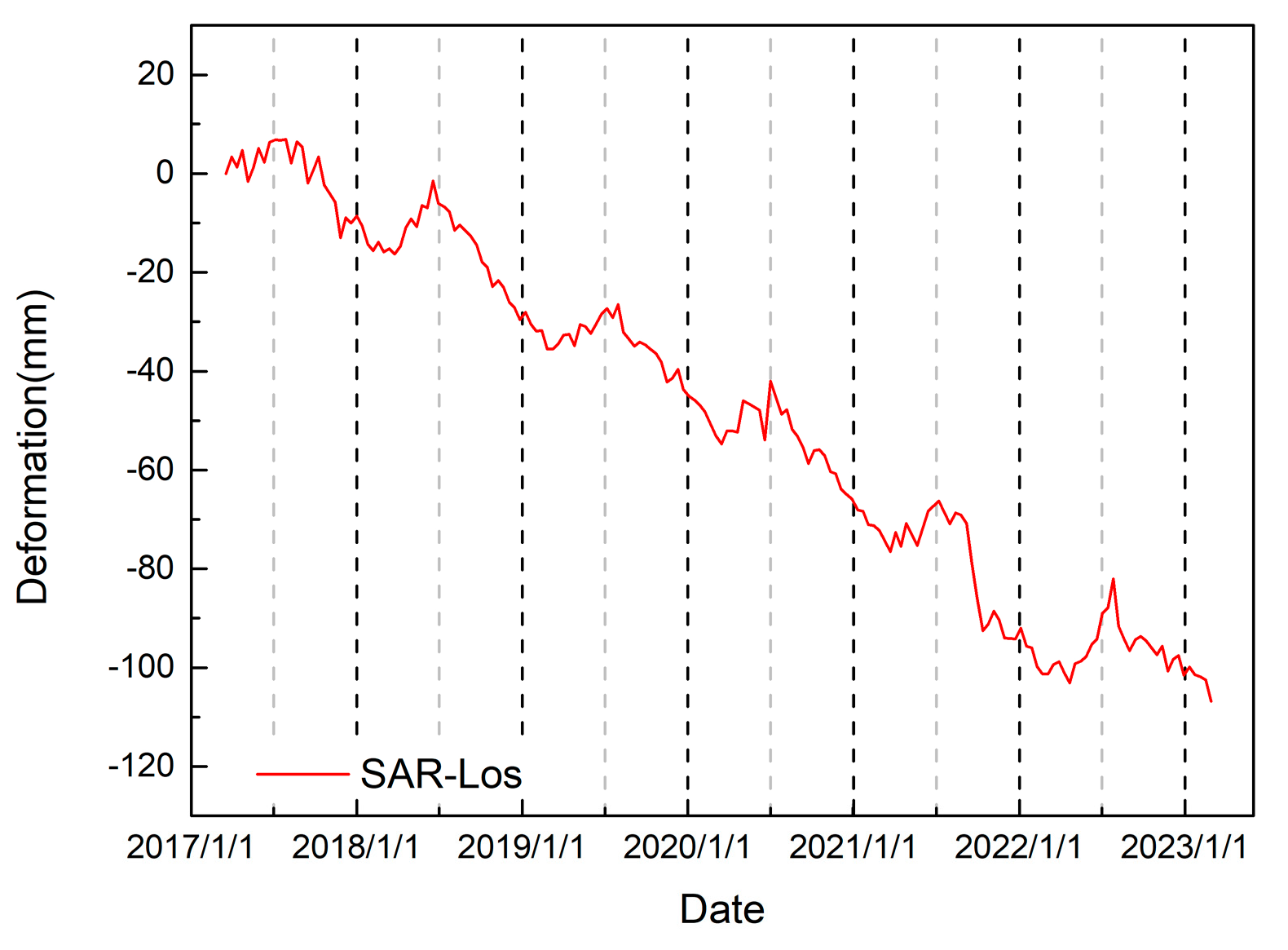
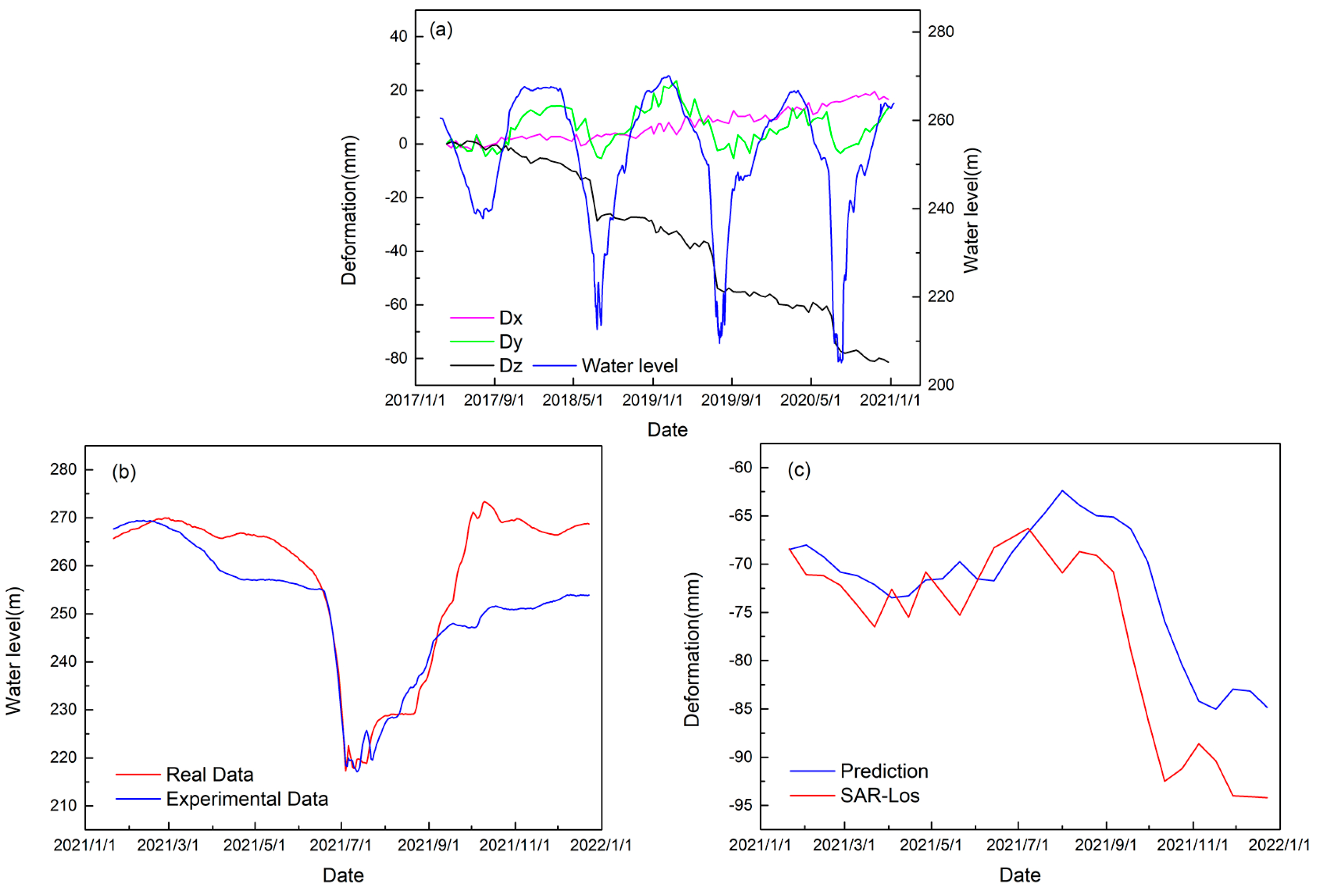
The true deformation of the dam obtained via the geodetic method at the typical point P is shown in Figure 11b. The dam field deformation monitoring dataset consists of a total of data in three directions, Dx, Dy, and Dz, acquired from March 2017 to December 2020. We projected the displacement data in three directions upward to the satellite’s line of sight according to the formula and compared them with the data obtained via InSAR, as shown in Figure 11c. The accuracy of the accumulated deformation value for P was 95%, and the correlation coefficient R was 0.93. We found that the data distributions of P and the InSAR deformation values were in good agreement.

Figure 11.
(a) Location of on-site data point P. (b,c) Measured data of ground point P; Dx, Dy, and Dz are measured on the ground in each of the three directions, Los is the deformation data Los after the projection of the measured data, and SAR-Los is data from the InSAR deformation model.
4.2. Analysis of Deformation and Water Storage Level Data
Based on the InSAR deformation model data SAR-Los analyzed above, the deformation of the dam was generally decreasing, but there was still a local trend of periodic changes. At the typical point P, the deformation curve had a localized upward trend around June each year, as shown in Figure 12.

Figure 12.
The schematic diagram of the periodicity of deformation at point P.
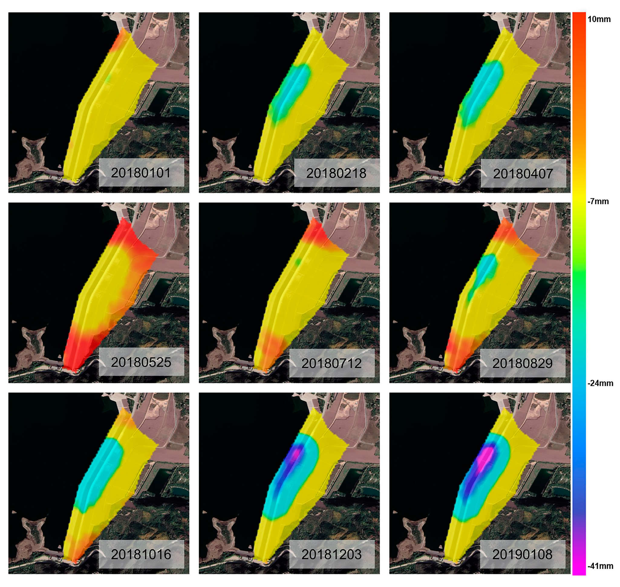
The overall deformation of the dam during 2018–2019 was specifically taken and plotted. As shown in Figure 13, only the center of the dam showed obvious periodic deformation throughout the year, and the overall deformation trends of the center of the dam and point P are the same. But there was basically no deformation on either side or the lower part of the dam. At this point, our conclusion is that the deformation of the dam body of the Xiaolangdi Dam is periodic.

Figure 13.
The time series variation of the cumulative deformation of Xiaolangdi Dam from 2018 to 2019.
Henan Province has a continental monsoon climate with a large amount of rain in the summer and little rain in the winter. In response to changes in precipitation, reservoir levels must also be adjusted. The water contact surface on the upstream side of the dam is subjected to hydrostatic pressure from the reservoir water. As the reservoir level changes, the hydrostatic pressure also changes. Considering that the Xiaolangdi Dam also exhibits a cyclic deformation trend, we speculate that hydrostatic pressure is the main driving factor for deformation.
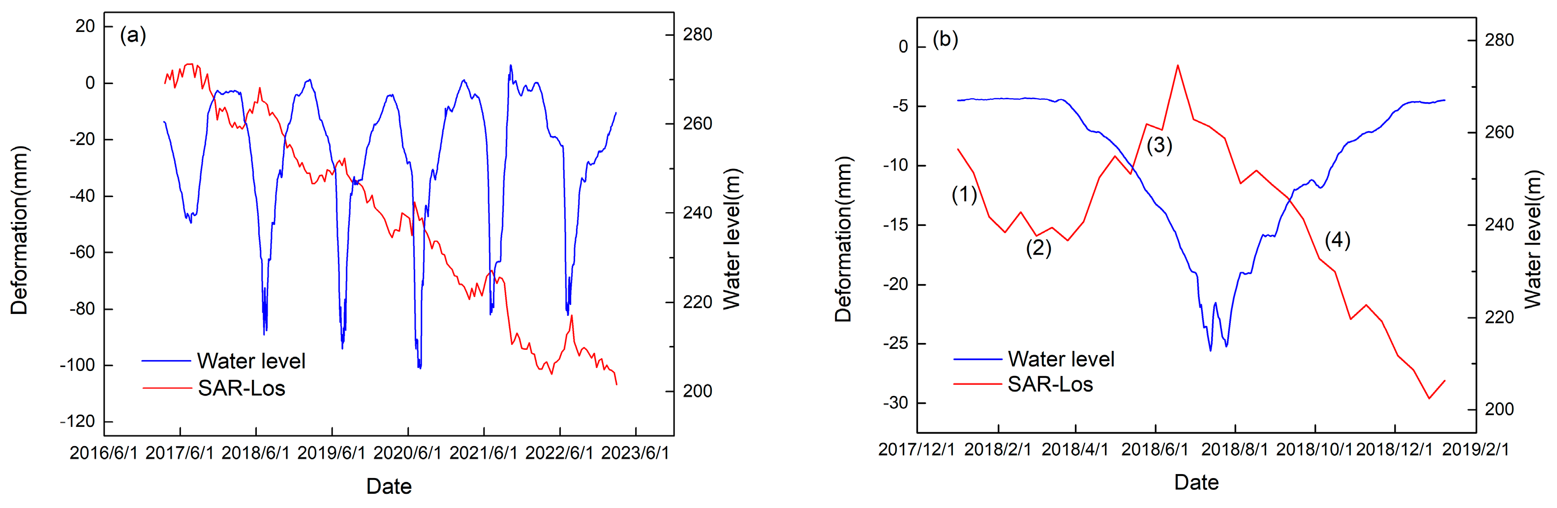
We compared the InSAR deformation data of the dam at the typical point P with the water level data, as shown in Figure 14. The Pearson correlation coefficient R between the accumulated deformation values of the InSAR model and the storage level data was 0.81. In order to express the relationship between the two more clearly, we selected the detailed comparison data of the storage level and deformation between 2018 and 2019 for analysis.
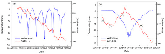
Figure 14.
(a) Comparison of deformation data and water storage level data at point P; (b) Stage diagram of deformation data and water storage level data in 2018–2019, (1)–(4) are the numbering of the different stages based on the trend of the line.
Over one year, the deformation curve can be roughly divided into four stages according to the slope of the curve, as shown in Figure 14b, and we performed a statistical analysis on the water storage level and deformation information in different stages, as shown in Table 1. By analyzing the relationship between the two, we concluded that around the field measuring point, the deformation value decreases when the water storage level increases and increases when the water storage level decreases around the typical point P.

Table 1.
The characteristics of the water storage level and dam deformation changes at different times.
4.3. Prediction of Deformation Based on Reservoir Water Level Data
The Xiaolangdi Dam is subject to periodic deformation owing to changes in the upstream reservoir level. The storage level and deformation showed a strong correlation.
In this study, data from in situ measurements were only available at the typical point P, and the monitoring period was short and irregular. In contrast, the InSAR deformation model has a large amount of data and a higher accuracy, which was verified by the data at the typical point P.
The time span of the InSAR data used in the time series deformation model was six years, with a total of 173 periods of deformation data and a total of 2386 points for each period of InSAR deformation data. After all data were interpolated, a total of 181 data periods were obtained, with an interval of 12 d between two data periods. Each InSAR deformation period corresponds to twelve days of daily reservoir level data.
The InSAR-LSTM deformation prediction model was built by taking the daily reservoir level data as input and the InSAR model deformation data as output. The data were divided into a training set and prediction set according to the time series, and the division results are shown in Table 2. The hyperparameter steps were applied in the model to combine the data, and after some debugging, the best step parameter was determined to be 2, which means that every two sets of two periods of connected data were combined, and the final ratio of the training set and the prediction set obtained was 164:13.
Table 2.
Distribution of training and prediction sets in the total data and their time spans.
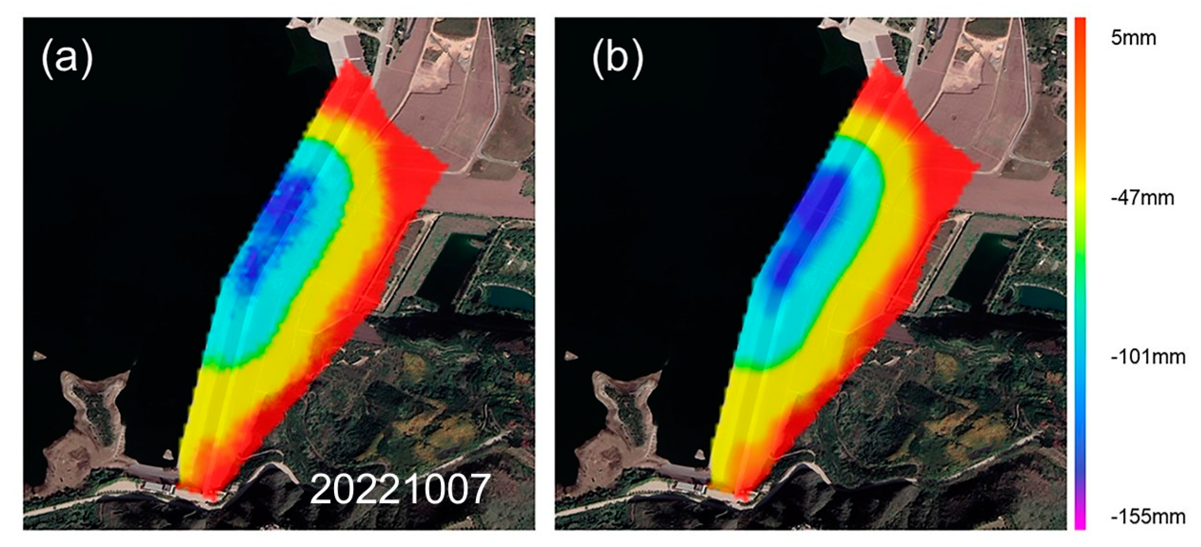
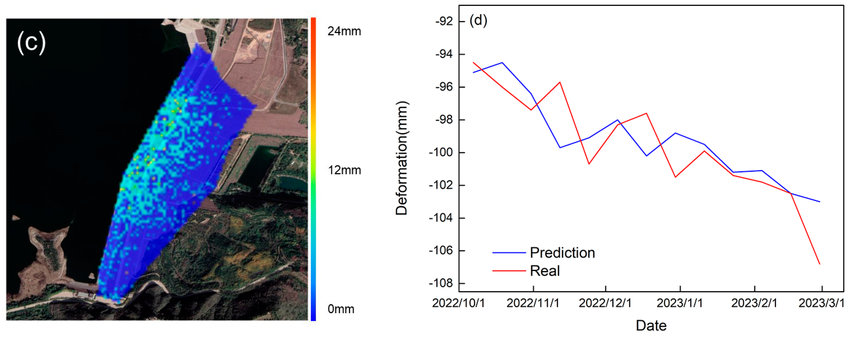
The LSTM model produced thirteen sets of predictions; Figure 15a shows the first period of data for the predicted results, which is the cumulative deformation data for the dam on 7 October 2022. Figure 15c shows the errors of the InSAR deformation data y and the prediction data , which are shown in Figure 15b. The error calculation index is MAE, which is calculated as in Equation (4); the relative error is still concentrated at 10 percent or less, and only some of the points of the absolute error reach 24 mm.


Figure 15.
(a) Prediction results deformation data. (b) InSAR model deformation data. (c) Error distribution of the MAE in the prediction results. The results of the remaining twelve forecasts are presented in the Supplementary document. (d) Comparison of deformation data and predicted results at point P.
At the typical point P, the comparison between the InSAR deformation data and the prediction data is shown in Figure 15d. There are thirteen periods of data for point P. The final cumulative deformation values for the InSAR deformation data and the predicted deformation data were −106.8 mm and −103 mm, respectively, and the relative accuracies were 96.4%. We used MAE, MSE, RMSE, and R as indicators for evaluating the overall prediction accuracy, which are calculated as shown in Equations (3)–(6). The calculation results are shown in Table 3.
Table 3.
Accuracy evaluation for four deformation prediction models.
4.4. Multimodel Comparison and Parameter Optimization
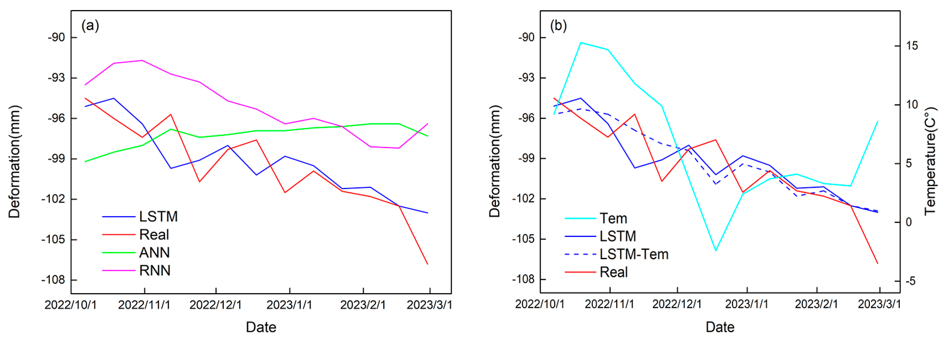
In Figure 16a, the prediction data of the ANN, RNN, and LSTM models are compared with the InSAR deformation data, and the accuracy evaluation indexes of each model are shown in Table 3. It can be seen that the LSTM model had the highest prediction accuracy and the ANN model had the lowest prediction accuracy, which proves that the LSTM model is more suitable for deformation prediction in this study.
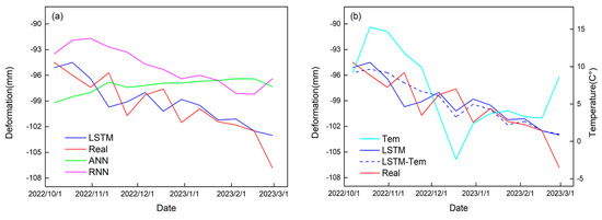
Figure 16.
(a) Comparison of the prediction data of the three models ANN, RNN and LSTM at typical point P. (b) Comparison of the prediction data before and after the addition of the temperature parameter to the LSTM model.
At present, researchers studying dam deformation commonly use the rheological deformation model, which is a real physical model. This approach requires a large number of dam-related parameters and a high level of professionalism on the part of the researcher [58].
The LSTM model is a mathematical model that can be modeled from a numerical point of view, but it does not take into account the real physical meaning of the numerical values in the calculation. In addition to hydrostatic pressure, environmental parameters such as temperature also have an effect on the deformation of the dam. We optimized the LSTM deformation prediction model using daily average temperature data.
Figure 16b shows the predicted data using the model with the added parameters compared to the data without the added parameters, and a comparison of the accuracy of the two sets of predicted and deformed data is shown in Table 3. From the accuracy index in the table, it can be seen that adding the temperature environment parameter to the LSTM deformation prediction model can make the prediction more closely match the deformation data.
5. Discussion
The main body of the dam sinks under the influence of its own gravity. In the case of a rockfill dam, which is constructed of rocks and sediment, the water stored in the reservoir percolates from upstream to downstream, creating a seepage field. The seepage field exerts uplift pressure on the bottom of the dam, which is equivalent to reducing the gravity of the dam. In addition, the reservoir impoundment exerts hydrostatic pressure on the contact surface between the dam and the water, and the dam will slowly move downstream, with a change in hydrostatic pressure and a change in the trend of movement.
The relationship between on-site measurement displacement and storage level in the three directions of the typical point P is shown in Figure 17a. The amount of displacement of point P to the left and right along the axis of the dam was relatively small and showed slow growth. In the downstream direction of the dam, the magnitude of the displacement was basically synchronized with the rise and fall of the storage level, but there was still a delay of about 20 days. In the vertical direction of the dam, an accelerated subsidence of point P occurred each year after the water level fell since the uplift pressure was reduced and slowly continued as the water level began to rise to its highest point. Compared with the vertical settlement, the displacement along the flow direction of the dam contributed to a larger part in the projection process. Therefore, in the process of moving away from the satellite platform, the dam shows a small rebound trend with a decrease in the storage water level, but the overall trend is away from the satellite platform.
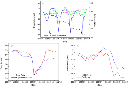
Figure 17.
(a) Relationship between on–site deformation data and storage level data at typical point P. (b,c) Comparison of the point P deformation values predicted using the simulated storage level experimental data with the InSAR model deformation values in 2021.
From the perspective of this study’s findings, if we want to reduce the deformation of the dam, we should try to avoid storing the reservoir at the highest level for a long period of time in order to mitigate the movement of the dam downstream, restore the water after the reservoir storage level decreases, use the uplift pressure to mitigate the effect of gravity on the settlement of the dam, and avoid the prolonged operation of the reservoir at a low water level.
The annual cumulative deformation value of point P in 2021 reached −25.9 mm, which is the maximum value of annual deformation in the whole monitored cycle. We made adjustments to the actual storage level in 2021 as described above, and Figure 15b shows a comparison of the simulated storage with the real storage level data after the optimization was performed. We used the optimized storage level experimental data as input into the deformation prediction model, and the results are shown in Figure 17c. At each of the 29 points shown in the figure, the average deformation weakening value was 4.9 mm. The final cumulative annual deformation value was −16.4 mm, which is an effective deformation reduction of about 37%.
The Xiaolangdi Water Conservancy Hub is a large-scale water conservancy facility, and effective reservoir storage management can extend the service life of the dam, and any changes to the reservoir level management program must be carefully considered before they are put into practice. In general, reservoir managers should follow a multifactorial approach to determine the reservoir’s storage level scheduling program, such as using actual river flow and weather data. When the weather is bad and the reservoir needs to be kept in operation at an extreme storage level, the model can also be used in advance to predict possible pitfalls and determine countermeasures.
6. Conclusions
The Xiaolangdi Dam was constructed more than 20 years ago, and the main body of the dam underwent deformation during 2017–2023, which was investigated in this study. A time series deformation model of the main body of the Xiaolangdi Dam was established using InSAR technology, which can accurately reflect the overall deformation information of the dam after verification using the measured data. By combining the ground truth data, the InSAR time series deformation model, and the LSTM deformation prediction model, we can conclude the following:
- The InSAR deformation model shows that there is a gradual weakening in the deformation trend of the dam from the center to the sides and from the top to the bottom. Throughout the 6-year deformation cycle, although there were differences in the deformation trends in different parts of the dam, each region was excessively smooth. The 6-year cumulative deformation in the middle part of the dam near the upstream reached -155 mm, which is within the safe range for large rockfill dams.
- The Xiaolangdi Dam continuously deforms. The satellite platform can continuously and periodically acquire InSAR image data, which helps monitor the overall deformation of the dam over a long period of time and allows more deformation information to be obtained. Theoretically, the combination of InSAR technology and the LSTM model can predict the effects of different storage level planning schemes on the dam and can then adjust storage level planning schemes in a targeted manner, attenuating dam deformation and preventing the risk of possible larger deformations.
- Owing to the inherent limitations of the satellite platform, ground-based measurement data are also required to verify the reliability of the deformation and prediction models. In the future, the launch of satellites with shorter revisit periods and higher resolutions could enable better monitoring of surface deformation. The specific mechanism by which hydrostatic pressure affects the structural stability of dams has not been studied in depth in this work, and this could be the subject of future research.
Supplementary Materials
The following supporting information can be downloaded at: https://www.mdpi.com/article/10.3390/w15193384/s1. Figure S1: Total dam deformation prediction results.
Author Contributions
Conceptualization, Z.F., Y.P. and R.H.; methodology, Z.F.; software, Z.F.; validation, Z.F. and H.Y.; formal analysis, R.H. and Y.P.; investigation, H.Y. and Z.H; resources, R.H.; data curation, Z.F.; writing—original draft preparation, Z.F.; writing—review and editing, R.H., Z.H., Y.P. and H.Y.; visualization, Z.F.; supervision, Z.H. and Y.P. All authors have read and agreed to the published version of the manuscript.
Funding
This work was supported by the State Key Project of the National Natural Science Foundation of China, Key Projects of Joint Funds for Regional Innovation and Development (grant number U22A20566); the Henan Provincial Higher Education Key Research Funding Project (grant number 18B420003); and the Henan University of Science and Technology Basic Research Business Expenses Specially Funded Project (grant number NSFRF170909).
Data Availability Statement
Santinel-1 image data and reservoir storage level data acquisition methods are mentioned in the Acknoledgments.
Acknowledgments
We sincerely thank the ESA for providing the Sentinel-1 data (https://search.asf.alaska.edu [accessed on 1 September 2023]), Guangqian Hu and Huijun Yang of the Xiaolangdi Engineering Consulting Co., Ltd., for compiling the measured data on the deformation of the Xiaolangdi Dam, and the Yellow River Network of the Yellow River Conservancy Commission of the Ministry of Water Resources of China for providing information on the storage level of the Xiaolangdi Reservoir (www.yrcc.gov.cn [accessed on 1 September 2023]).
Conflicts of Interest
The authors declare no conflict of interest.
References
- Ilyushin, Y.V.; Kapostey, E.I. Developing a Comprehensive Mathematical Model for Aluminium Production in a Soderberg Electrolyser. Energies 2023, 16, 6313. [Google Scholar] [CrossRef]
- Pershin, I.M.; Papush, E.G.; Kukharova, T.V.; Utkin, V.A. Modeling of Distributed Control System for Network of Mineral Water Wells. Water 2023, 15, 2289. [Google Scholar] [CrossRef]
- Wang, Q.Q.; Huang, Q.H.; He, N.; He, B.; Wang, Z.C.; Wang, Y.A. Displacement monitoring of upper Atbara dam based on time series InSAR. Surv. Rev. 2020, 52, 485–496. [Google Scholar] [CrossRef]
- Milillo, P.; Perissin, D.; Salzer, J.T.; Lundgren, P.; Lacava, G.; Milillo, G.; Serio, C. Monitoring dam structural health from space: Insights from novel InSAR techniques and multi-parametric modeling applied to the Pertusillo dam Basilicata, Italy. Int. J. Appl. Earth Obs. Geoinf. 2016, 52, 221–229. [Google Scholar] [CrossRef]
- Rotta, L.H.S.; Alcântara, E.; Park, E.; Negri, R.G.; Lin, Y.N.; Bernardo, N.; Mendes, T.S.G.; Filho, C.R.S. The 2019 Brumadinho tailings dam collapse: Possible cause and impacts of the worst human and environmental disaster in Brazil. Int. J. Appl. Earth Obs. Geoinf. 2020, 90, 102119. [Google Scholar]
- Gikas, V.; Sakellariou, M. Settlement analysis of the Mornos earth dam (Greece): Evidence from numerical modeling and geodetic monitoring. Eng. Struct. 2008, 30, 3074–3081. [Google Scholar] [CrossRef]
- Xi, R.; Liang, Y.; Chen, Q.; Jiang, W.; Chen, Y.; Liu, S. Analysis of Annual Deformation Characteristics of Xilongchi Dam Using Historical GPS Observations. Remote Sens. 2022, 14, 4018. [Google Scholar] [CrossRef]
- Chen, Z.; Yin, Y.; Yu, J.; Cheng, X.; Zhang, D.; Li, Q. Internal deformation monitoring for earth-rockfill dam via high-precision flexible pipeline measurements. Autom. Constr. 2022, 136, 104177. [Google Scholar] [CrossRef]
- Yao, F.H.; Guan, S.H.; Yang, H.; Chen, Y.; Qiu, H.F.; Ma, G.; Liu, Q.W. Long-term deformation analysis of Shuibuya concrete face rockfill dam based on response surface method and improved genetic algorithm. Water Sci. Eng. 2019, 12, 196–204. [Google Scholar] [CrossRef]
- Ma, C.; Yang, J.; Cheng, L.; Ran, L. Adaptive parameter inversion analysis method of rockfill dam based on harmony search algorithm and mixed multi-output relevance vector machine. Eng. Comput. 2020, 37, 2229–2249. [Google Scholar] [CrossRef]
- Xue, F.; Lv, X.; Dou, F.; Yun, Y. A Review of Time-Series Interferometric SAR Techniques: A Tutorial for Surface Deformation Analysis. IEEE Geosci. Remote Sens. Mag. 2020, 8, 22–42. [Google Scholar] [CrossRef]
- Li, B.; Li, Y.; Jiang, W.; Su, Z.; Shen, W. Conjugate ruptures and seismotectonic implications of the 2019 Mindanao earthquake sequence inferred from Sentinel-1 InSAR data. Int. J. Appl. Earth Obs. Geoinf. 2020, 90, 102127. [Google Scholar] [CrossRef]
- Yang, Y.; Chen, Q.; Xu, Q.; Zhang, Y.; Yong, Q.; Liu, G. Coseismic surface deformation of the 2014 Napa earthquake mapped by Sentinel-1A SAR and accuracy assessment with COSMO-SkyMed and GPS data as cross validation. Int. J. Digit. Earth 2017, 10, 1197–1213. [Google Scholar] [CrossRef]
- Noviello, C.; Verde, S.; Zamparelli, V.; Fornaro, G.; Pauciullo, A.; Reale, D.; Nicodemo, G.; Ferlisi, S.; Gulla, G.; Peduto, D. Monitoring Buildings at Landslide Risk With SAR: A Methodology Based on the Use of Multipass Interferometric Data. IEEE Geosci. Remote Sens. Mag. 2020, 8, 91–119. [Google Scholar] [CrossRef]
- Rodríguez, Á.B.; Balestriero, R.; De Angelis, S.; Benítez, M.C.; Zuccarello, L.; Baraniuk, R.; Ibanez, J.M.; de Hoop, M.V. Recurrent Scattering Network Detects Metastable Behavior in Polyphonic Seismo-Volcanic Signals for Volcano Eruption Forecasting. IEEE Trans. Geosci. Remote Sens. 2022, 60, 5909123. [Google Scholar]
- An, B.; Jiang, Y.; Wang, C.; Shen, P.; Song, T.; Hu, C.; Liu, K. Ground infrastructure monitoring in coastal areas using time-series inSAR technology: The case study of Pudong International Airport, Shanghai. Int. J. Digit. Earth 2023, 16, 2171144. [Google Scholar] [CrossRef]
- Shi, X.; Zhu, T.; Tang, W.; Jiang, M.; Jiang, H.; Yang, C.; Zhan, W.; Ming, Z.; Zhang, S. Inferring decelerated land subsidence and groundwater storage dynamics in Tianjin–Langfang using Sentinel-1 InSAR. Int. J. Digit. Earth 2022, 15, 1526–1546. [Google Scholar] [CrossRef]
- Pawłuszek-Filipiak, K.; Wielgocka, N.; Tondaś, D.; Borkowski, A. Monitoring nonlinear and fast deformation caused by underground mining exploitation using multi-temporal Sentinel-1 radar interferometry and corner reflectors: Application, validation and processing obstacles. Int. J. Digit. Earth 2023, 16, 251–271. [Google Scholar] [CrossRef]
- Yang, Z.; Xu, B.; Li, Z.; Wu, L.; Zhu, J. Prediction of Mining-Induced Kinematic 3-D Displacements from InSAR Using a Weibull Model and a Kalman Filter. IEEE Trans. Geosci. Remote Sens. 2022, 60, 4500912. [Google Scholar] [CrossRef]
- Liu, L.; Yu, J.; Chen, B.; Wang, Y. Urban subsidence monitoring by SBAS-InSAR technique with multi-platform SAR images: A case study of Beijing Plain, China. Eur. J. Remote Sens. 2020, 53 (Suppl. 1), 141–153. [Google Scholar] [CrossRef]
- Xing, X.; Zhu, Y.; Xu, W.; Peng, W.; Yuan, Z. Measuring Subsidence Over Soft Clay Highways Using a Novel Time-Series InSAR Deformation Model with an Emphasis on Rheological Properties and Environmental Factors (NREM). IEEE Trans. Geosci. Remote Sens. 2022, 60, 4601319. [Google Scholar] [CrossRef]
- Xing, X.; Huang, L.; He, Z.; Zhang, T.; Zhu, Y. Health Observation of the Capital Airport South Expressway Based on Improved MT-InSAR Technology. IEEE J. Miniaturization Air Space Syst. 2023, 4, 232–241. [Google Scholar] [CrossRef]
- Tang, W.; Motagh, M.; Zhan, W. Monitoring active open-pit mine stability in the Rhenish coalfields of Germany using a coherence-based SBAS method. Int. J. Appl. Earth Obs. Geoinf. 2020, 93, 102217. [Google Scholar] [CrossRef]
- Fan, H.; Li, T.; Gao, Y.; Deng, K.; Wu, H. Characteristics inversion of underground goaf based on InSAR techniques and PIM. Int. J. Appl. Earth Obs. Geoinf. 2021, 103, 102526. [Google Scholar] [CrossRef]
- Wang, Q.; Fan, J.; Zhou, W.; Tong, L.; Guo, Z.; Liu, G.; Yuan, W.; Sousa, J.J.; Perski, Z. 3D Surface velocity retrieval of mountain glacier using an offset tracking technique applied to ascending and descending SAR constellation data: A case study of the Yiga Glacier. Int. J. Digit. Earth 2019, 12, 614–624. [Google Scholar] [CrossRef]
- Li, Z.; Wu, Q. Capturing the crack process of the Antarctic A74 iceberg with Sentinel-1 based offset tracking and radar interferometry techniques. Int. J. Digit. Earth 2022, 15, 397–415. [Google Scholar] [CrossRef]
- Zhang, Z.; Lin, H.; Wang, M.; Liu, X.; Chen, Q.; Wang, C.; Zhang, H. A Review of Satellite Synthetic Aperture Radar Interferometry Applications in Permafrost Regions: Current status, challenges, and trends. IEEE Geosci. Remote Sens. Mag. 2022, 10, 93–114. [Google Scholar] [CrossRef]
- Zhou, W.; Li, S.; Zhou, Z.; Chang, X. InSAR Observation and Numerical Modeling of the Earth-Dam Displacement of Shuibuya Dam (China). Remote Sens. 2016, 8, 877. [Google Scholar] [CrossRef]
- Zhou, W.; Li, S.; Zhou, Z.; Chang, X. Remote Sensing of Deformation of a High Concrete-Faced Rockfill Dam Using InSAR: A Study of the Shuibuya Dam, China. Remote Sens. 2016, 8, 255. [Google Scholar] [CrossRef]
- Ruiz-Armenteros, A.M.; Marchamalo-Sacrsitán, M.; Bakoň, M.; Lamas-Fernández, F.; Delgado, J.M.; Sánchez-Ballesteros, V.; Papco, J.; González-Rodrigo, B.; Lazecky, M.; Perissin, D.; et al. Monitoring of an embankment dam in southern Spain based on Sentinel-1 Time-series InSAR. Procedia Comput. Sci. 2021, 181, 353–359. [Google Scholar] [CrossRef]
- Biondi, F.; Addabbo, P.; Clemente, C.; Ullo, S.L.; Orlando, D. Monitoring of Critical Infrastructures by Micromotion Estimation: The Mosul Dam Destabilization. IEEE J. Sel. Top. Appl. Earth Obs. Remote Sens. 2020, 13, 6337–6351. [Google Scholar] [CrossRef]
- Xiao, R.; Jiang, M.; Li, Z.; He, X. New insights into the 2020 Sardoba dam failure in Uzbekistan from Earth observation. Int. J. Appl. Earth Obs. Geoinf. 2022, 107, 102705. [Google Scholar] [CrossRef]
- Bayik, C.; Abdikan, S.; Arıkan, M. Long term displacement observation of the Atatürk Dam, Turkey by multi-temporal InSAR analysis. Acta Astronaut. 2021, 189, 483–491. [Google Scholar] [CrossRef]
- Hochreiter, S.; Schmidhuber, J. Long Short-Term Memory. Neural Comput. 1997, 9, 1735–1780. [Google Scholar] [CrossRef] [PubMed]
- Senanayake, S.; Pradhan, B.; Alamri, A.; Park, H.-J. A new application of deep neural network (LSTM) and RUSLE models in soil erosion prediction. Sci. Total Environ. 2022, 845, 157220. [Google Scholar] [CrossRef] [PubMed]
- Dikshit, A.; Pradhan, B.; Alamri, A.M. Pathways and challenges of the application of artificial intelligence to geohazards modelling. Gondwana Res. 2021, 100, 290–301. [Google Scholar] [CrossRef]
- Guo, Y.; Yu, X.; Xu, Y.-P.; Chen, H.; Gu, H.; Xie, J. AI-based techniques for multi-step streamflow forecasts: Application for multi-objective reservoir operation optimization and performance assessment. Hydrol. Earth Syst. Sci. 2021, 25, 5951–5979. [Google Scholar] [CrossRef]
- Huang, B.; Kang, F.; Li, J.; Wang, F. Displacement prediction model for high arch dams using long short-term memory based encoder-decoder with dual-stage attention considering measured dam temperature. Eng. Struct. 2023, 280, 115686. [Google Scholar] [CrossRef]
- Jena, R.; Naik, S.P.; Pradhan, B.; Beydoun, G.; Park, H.-J.; Alamri, A. Earthquake vulnerability assessment for the Indian subcontinent using the Long Short-Term Memory model (LSTM). Int. J. Disaster Risk Reduct. 2021, 66, 102642. [Google Scholar] [CrossRef]
- Li, H.; Xu, Q.; He, Y.; Fan, X.; Yang, H.; Li, S. Temporal detection of sharp landslide deformation with ensemble-based LSTM-RNNs and Hurst exponent. Geomat. Nat. Hazards Risk 2021, 12, 3089–3113. [Google Scholar] [CrossRef]
- Chen, C.; Zhang, Q.; Kashani, M.H.; Jun, C.; Bateni, S.M.; Band, S.S.; Dash, S.S.; Chau, K.W. Forecast of rainfall distribution based on fixed sliding window long short-term memory. Eng. Appl. Comput. Fluid Mech. 2022, 16, 248–261. [Google Scholar] [CrossRef]
- Radman, A.; Akhoondzadeh, M.; Hosseiny, B. Integrating InSAR and deep-learning for modeling and predicting subsidence over the adjacent area of Lake Urmia, Iran. GISci. Remote Sens. 2021, 58, 1413–1433. [Google Scholar] [CrossRef]
- Zebker, H.; Werner, C.; Rosen, P.; Hensley, S. Accuracy of topographic maps derived from ERS-1 interferometric radar. IEEE Trans. Geosci. Remote Sens. 1994, 32, 823–836. [Google Scholar] [CrossRef]
- Zhang, Z.; Zeng, Q.; Jiao, J. Application of D-InSAR Technology on Risk Assessment of Mining Area. In Proceedings of the IGARSS 2019–2019 IEEE International Geoscience and Remote Sensing Symposium, Yokohama, Japan, 28 July–2 August 2019; pp. 9695–9698. [Google Scholar]
- Lanari, R.; Mora, O.; Manunta, M.; Mallorqui, J.; Berardino, P.; Sansosti, E. A small-baseline approach for investigating deformations on full-resolution differential SAR interferograms. IEEE Trans. Geosci. Remote Sens. 2004, 42, 1377–1386. [Google Scholar] [CrossRef]
- Hooper, A.; Prata, F.; Sigmundsson, F. Remote Sensing of Volcanic Hazards and Their Precursors. Proc. IEEE 2012, 100, 2908–2930. [Google Scholar] [CrossRef]
- Ferretti, A.; Prati, C.; Rocca, F. Permanent scatterers in SAR interferometry. IEEE Trans. Geosci. Remote Sens. 2001, 39, 8–20. [Google Scholar] [CrossRef]
- Ferretti, A.; Prati, C.; Rocca, F. Nonlinear subsidence rate estimation using permanent scatterers in differential SAR interferometry. IEEE Trans. Geosci. Remote Sens. 2000, 38, 2202–2212. [Google Scholar] [CrossRef]
- Berardino, P.; Fornaro, G.; Lanari, R.; Sansosti, E. A new algorithm for surface deformation monitoring based on small baseline differential SAR interferograms. IEEE Trans. Geosci. Remote Sens. 2002, 40, 2375–2383. [Google Scholar] [CrossRef]
- Liu, G.; Buckley, S.M.; Ding, X.; Chen, Q.; Luo, X. Estimating Spatiotemporal Ground Deformation with Improved Permanent-Scatterer Radar Interferometry. IEEE Trans. Geosci. Remote Sens. 2009, 47, 2762–2772. [Google Scholar] [CrossRef]
- Tao, Q.; Wang, F.; Guo, Z.; Hu, L.; Yang, C.; Liu, T. Accuracy verification and evaluation of small baseline subset (SBAS) interferometric synthetic aperture radar (InSAR) for monitoring mining subsidence. Eur. J. Remote Sens. 2021, 54, 642–663. [Google Scholar] [CrossRef]
- Pepe, A.; Euillades, L.D.; Manunta, M.; Lanari, R. New Advances of the Extended Minimum Cost Flow Phase Unwrapping Algorithm for SBAS-DInSAR Analysis at Full Spatial Resolution. IEEE Trans. Geosci. Remote Sens. 2011, 49, 4062–4079. [Google Scholar] [CrossRef]
- Chen, F.; Zhou, W.; Tang, Y.; Li, R.; Lin, H.; Balz, T.; Luo, J.; Shi, P.; Zhu, M.; Fang, C. Remote sensing-based deformation monitoring of pagodas at the Bagan cultural heritage site, Myanmar. Int. J. Digit. Earth 2022, 15, 770–788. [Google Scholar] [CrossRef]
- Song, R.; Guo, H.; Liu, G.; Perski, Z.; Yue, H.; Han, C.; Fan, J. Improved Goldstein SAR Interferogram Filter Based on Adaptive-Neighborhood Technique. IEEE Geosci. Remote Sens. Lett. 2015, 12, 140–144. [Google Scholar] [CrossRef]
- Hu, J.; Li, Z.-W.; Sun, Q.; Zhu, J.-J.; Ding, X.-L. Three-Dimensional Surface Displacements from InSAR and GPS Measurements With Variance Component Estimation. IEEE Geosci. Remote Sens. Lett. 2012, 9, 754–758. [Google Scholar]
- LeCun, Y.; Bengio, Y.; Hinton, G. Deep learning. Nature 2015, 521, 436–444. [Google Scholar] [CrossRef]
- Chiang, Y.-M.; Hao, R.-N.; Xu, Y.-P.; Liu, L. Multi-source rainfall merging and reservoir inflow forecasting by ensemble technique and artificial intelligence. J. Hydrol. Reg. Stud. 2022, 44, 101204. [Google Scholar] [CrossRef]
- Qiu, Z.; Cao, T.; Li, Y.; Wang, J.; Chen, Y. Rheological Behavior and Modeling of a Crushed Sandstone-Mudstone Particle Mixture. Processes 2018, 6, 192. [Google Scholar] [CrossRef]


Disclaimer/Publisher’s Note: The statements, opinions and data contained in all publications are solely those of the individual author(s) and contributor(s) and not of MDPI and/or the editor(s). MDPI and/or the editor(s) disclaim responsibility for any injury to people or property resulting from any ideas, methods, instructions or products referred to in the content. |
© 2023 by the authors. Licensee MDPI, Basel, Switzerland. This article is an open access article distributed under the terms and conditions of the Creative Commons Attribution (CC BY) license (https://creativecommons.org/licenses/by/4.0/).