Article

Forecasting Snowmelt Season Temperatures in the Mountainous Area of Northern Xinjiang of China

1
College of Geography and Remote Sensing Sciences, XinJiang University, Urumqi 830017, China
2
Xinjiang Xingnong Net Information Center, Urumqi 830002, China
3
Institute of Desert Meteorology, China Meteorological Administration, Urumqi 830002, China
4
Xinjiang Education Management Information Center, Urumqi 830049, China
5
Koktokay Snow Station, State Key Laboratory of Cryospheric Science, Northwest Institute of Eco-Environment and Resources, Chinese Academy of Sciences, Lanzhou 730000, China
6
XinJiang Meteorological Observatory, Urumqi 830002, China
*
Author to whom correspondence should be addressed.
Water 2023, 15(19), 3337; https://doi.org/10.3390/w15193337
Submission received: 23 August 2023 / Revised: 20 September 2023 / Accepted: 21 September 2023 / Published: 22 September 2023

Abstract

:
The mountains in northern Xinjiang of China were studied during the snowmelt season. Multi-source fusions of live data of the Chinese Land Data Assimilation System (CLDAS, 0.05° × 0.05°, hourly data) were used as real data, and the Central Meteorological Observatory guidance forecast (SCMOC, 0.05° × 0.05°, forecasting the following 10 days in 3 h intervals) was used as forecast data, both of which were issued by the China Meteorological Administration. The dynamic linear regression and the average filter correction algorithms were selected to revise the original forecast products for SCMOC. Based on the conventional temperature forecast information, we designed four temperature-rise prediction algorithms for essential factors affecting snowmelt. The temperature-rise prediction algorithms included the daily maximum temperature algorithm, daily temperature-rise-range algorithm, snowmelt temperature algorithm, and daily snowmelt duration algorithm. Four temperature-rise prediction values were calculated for each prediction product. The root–mean-squared error algorithm and temperature prediction accuracy algorithm were used to compare and test each prediction algorithm value from the time sequence and spatial distribution. Comprehensive tests showed that the forecast product revised by the average filter algorithm was superior to the revised dynamic linear regression algorithm as well as the original forecast product. Through these algorithms, the more suitable temperature-rise forecast value for each grid point in the study area could be obtained at different prediction times. The comprehensive and accurate temperature forecast value in the mountainous snowmelt season could provide an accurate theoretical basis for the effective prediction of runoff in snowmelt areas and the prevention of snowmelt flooding.

1. Introduction

Northern Xinjiang is one of the three areas with seasonal snow cover in China [1,2,3]. The snow cover on the Ertysi River basin is particularly deep in winter, where the source area snow depth reached 197 cm during the winter of 2021/2022. In northern Xinjiang, seasonal snowmelt water is the main local water resource, and the snowmelt runoff can supply more than 75% of rivers in spring [4,5]. The temperature variation in the mountains in spring is the major determining factor of the snowmelt runoff formation and the snowmelt flood occurrence [6,7,8,9]. The positive temperature change was more favorable for snow ablation [10,11]. An analysis based on the annual maximum flood peak records in the last 50 years and the frequency of the warming snowmelt (ice) floods in the last 20 years in Xinjiang indicated that rising temperatures in the mountains had led to the early melting of the glaciers in the surrounding areas [12,13,14]. The continuous rapid rise of the temperatures caused the snowmelt floods in Xinjiang [15]. The temperature had an important element of snowmelt [16]. Several studies made dynamic evaluations and forecasts on the occurrence of snowmelt flooding in spring [17,18,19]. All of these analyses have confirmed a direct relationship between the snowmelt and the temperature, with all research based on data from the meteorological observation stations. The distances between the meteorological observation stations in Xinjiang were several hundred kilometers, and there are even fewer observation stations in mountainous areas. Thus, the station data alone cannot quickly and accurately characterize the temperature changes in mountainous areas. SCMOC, a grid forecasting product (0.05° × 0.05°, forecasting the following 10 days in 3 h intervals), was used in this study to carry out full-coverage forecasts for the mountainous areas, and data were stable where services had been delivered. However, this forecast product had an average temperature forecast accuracy of less than 50% in mountainous areas. Therefore, it was necessary to design a correction algorithm to improve the accuracy of the original forecast product in mountainous areas.
Numerous studies have shown that numerical weather predictions provided early warnings with extended lead time [20,21,22,23] and improved the reservoir’s flood control and water supply objectives [24,25,26]. In catchments with seasonal snow cover, snowmelt is an important flood-generating process. Hence, high-quality air temperature data have been important to accurately forecast streamflow [27]. In recent years, intelligent grid-point temperature-prediction technology has become an important field, and numerous scholars have studied localized correction algorithms to improve the accuracy of local temperature forecasting in real time [28,29,30,31]. Dai et al. used a unary linear regression algorithm and a Kriging interpolation algorithm [32], and Hao et al. used a sliding training algorithm and an optimized variable-weights algorithm [33] to train the temperature data of the ECMWF fine-grid forecast products [34]. Wei et al. and Wan et al. tested and evaluated the products of the intelligent grid-prediction (SCMOC) service and the ECMWF fine-grid service, respectively [35,36]. Li et al. established three forecast models, including horizontal, longitudinal, and horizontal/longitudinal integrated forecast models [37], and Liu et al. used three algorithms including wavelet analysis, a sliding training algorithm, and an optimal fusion algorithm [38] to correct the temperature forecast products (SCMOC). Their analyses results showed that these algorithms were partially able to revise the temperature predictions in their study area. However, few of these revision algorithms considered mountain areas, which specifically forecast the future temperature of the snowmelt and snowmelt temperature-rise range. Due to the lack of meteorological observation data in mountainous areas, the physical weather processes have been unpredictable, and the numerical prediction models have been unable to account for the steep and complex terrain, making temperature forecasts in mountainous areas difficult. The prediction accuracy of the temperature in mountainous areas is lower than the temperatures of the plains. Therefore, improving the accuracy of the temperature forecasts in the mountainous areas is of the utmost importance.
In this study, two aspects were considered to design the correction algorithms. First, the mountainous terrain is steep, and the temperature changes dramatically with increasing altitude. We designed a dynamic linear regression algorithm, and the latest real values were used to dynamically update the slope of the regression equation of the temperature prediction in order to forecast the temperature changes. Secondly, the amount of the grid data and the system forecast errors in the mountainous area were significant. Therefore, we designed an average filter-correction algorithm that used the latest real values to dynamically update the forecast errors for different forecast periods to predict the temperatures in the mountainous area.
In this research, we studied the intelligent grid temperature prediction technology of the temperature rise during the spring snowmelt period in the mountainous area of northern Xinjiang. Two temperature prediction correction algorithms were designed to correct the original forecast product SCMOC. After correction, two new forecast products were obtained. In order to focus on the influence of temperature-rise prediction accuracy during the spring snowmelt period based on the temperature forecast information, four innovative temperature-rise prediction algorithms were designed to more accurately describe the physical quantity index of the snowmelt process. The temperature-rise prediction algorithms included prediction algorithms for the daily maximum temperature, daily temperature-rise range, snowmelt temperature, and daily snowmelt duration. The values of four temperature-rise prediction algorithms for each forecast product were calculated. Though multiple indexes were used to compare and test the value of each temperature-rise prediction algorithm and the temperature prediction from the time sequence and spatial distribution, a suitable forecast product was selected for mountainous areas.

2. Data and Methods

The study area included mountainous areas with altitudes above 1300 m in northern Xinjiang, ranging from 42.25° to 49.20° N and 79.85° to 96.50° E, with a total of 7371 grid points and a spatial resolution of 0.05° × 0.05°, as shown in Figure 1.
There were three temperature forecast products, which included the original product (the product research area was in Xinjiang, shortened to XJ) that was obtained from the temperature guidance forecast product of the China Meteorological Administration (SCMOC); the revised product (translated into Chinese Pinyin HuiGui, shortened to HG) that used the original forecast product modified by the dynamic linear regression algorithm; the revised product (translated into Chinese pinyin PinJun, shortened to PJ) that used the original forecast product modified by the average filter correction algorithm. The temperature forecast products predicted future values at 240 h in 3 h interval values with a spatial resolution of 0.05° × 0.05°, and their reports started at 08:00 (Beijing time), every day, from March to May 2021.
Real data were simulated values, which were obtained from Chinese Land Data Assimilation System (CLDAS) hourly data with a spatial resolution of 0.05° × 0.05°. The advantage of the real product was the combination of multi-source fusion data, such as ground observation data, ECMWF numerical product, GFS numerical product, Fengyun-2 weather satellite precipitation product, Fengyun-2 weather satellite full disk nominal map, and digital elevation model data. After evaluation by the Meteorological Information Center of China, the temperature of CLDAS was in good agreement with the actual ground observation values [39]. After Liu Ying et al. evaluated the temperatures of CLDAS-V2.0 in northwest China, including this study area, the test results of CLDAS showed that the non-independent test was 0.972, the independent test was 0.950, the mean deviation was −0.271 °C, the RMSE was 2.406 °C, and the mean absolute error was 1.588 °C [40].

2.1. Temperature Revision Method

2.1.1. Dynamic Unitary Linear Regression (HG) Revision Scheme

Based on the temperature forecast products (XJ) in the mountainous area of northern Xinjiang, in spring, from March to May 2021, the unary regression correction model was established by each grid and each forecast period dynamically, and a new forecast data product (HG) was generated after each revision. The revised model formula of the dynamic regression equation was as follows:
b = j = 1 d n X ( d i ) Y ( d i ) n x ¯ y ¯ i = 1 d n X ( d i ) 2 n x ¯ 2 ,
a = y ¯ b x ¯ ,
Y = a X + b ,
The forecast value of one grid at the forecast period on the day was revised by the following steps. In Equation (1), n represents the number of days of dynamic training in the previous days, according to previous experiments on observation stations, and n = 6 was chosen in this paper, where x represents the temperature forecast value (XJ) and y represents the actual value of the corresponding time, d represents the day the forecast began, i stands for integer value 1 − n, (d − i) indicates the previous i day, x ¯ represents the temperature forecast average value (XJ), and y ¯ represents the average actual value of the corresponding time. Equation (1) calculated the value of b. According to x ¯ , y ¯ , and b calculated by Equation (1), the value of a was calculated by Equation (2). In Equation (3), X is the original forecast value (XJ), and Y is the forecast value after regression correction (HG). According to b of Equation (1) and a of Equation (2), the correction value Y was computed by Equation (3).
There were 7371 grid points in this study area. One grid point had forecast the following 240 h in 3 h intervals every day, yielding 80 forecast values per day. Each grid forecast value was revised according to the above steps.

2.1.2. Average Filtering (PJ) Revision Scheme

Both the original temperature forecast product (XJ) and the real product CLDAS were grid data with a spatial resolution of 0.05° × 0.05°. The average filtering algorithm was used to correct the original forecast temperature, and the revised temperature forecast product, marked as PJ, was obtained. The forecast value of one grid at the forecast period on the day, as revised by average filtering algorithm, is as follows:
① Calculation of model prediction error:
b ( d ) = f ( d ) a ( d ) ,
In Equation (4): b(d) is the prediction error value, which was defined as the prediction error between the prediction data f(d) of a certain prediction time and the corresponding live data a(d).
② Daily sliding forecast error model:
B ( d ) = b ( d 1 ) + b ( d 2 ) + ... + b ( d n ) n ,
In Equation (5): B(d) is the corrected error of the model forecast, which was the arithmetic average of the temperature forecast error of the same grid at the same forecast period every day for n days before the forecasting date. Through numerous experiments conducted by meteorological observation stations in different regions, different values of n were found to have great influence on B(d). Based on previous periodic studies and reference materials [29], this study selected n = 6.
③ Model forecast error revision:
F ( d ) = f ( d ) B ( d ) ,
In Equation (6), B(d) was obtained by Equation (5), f(d) is the forecast value of the original temperature forecast product (XJ), and F(d) is the revised forecast value.
Equations (4)–(6) referred to the process of correcting specific forecast periods of the same grid. Equations (4)–(6) were used to correct the temperature for every forecast period of 7371 grid points in mountainous areas. After the correction, a new temperature forecast product (PJ) at 3 h intervals for the following 10 days, forecasted from 8 a.m. every day, was generated.

2.2. Temperature Forecast Method

2.2.1. Forecast of Daily Maximum Temperature

In the forecast for the next 10 days in 3 h intervals at 08:00 (Beijing time) every day, the maximum temperature was selected as the daily maximum temperature forecast value according to the 8 forecast periods of each 24 h interval, such as 0–24 h and 24–48 h, and the daily maximum temperature forecast values in the future for 1–10 days (d) were calculated similarly. The method for selecting the real maximum temperature was the same. The daily maximum temperature was selected from the corresponding eight real values of the forecast obtained during the day.

2.2.2. Forecast of Temperature-Rise Range

First, the daily maximum temperature of grid points was calculated, followed by the daily temperature-rise range during the temperature-rise period.
U P i = H o u i Q i a n i ,
U P s k = H o u s k Q i a n s k ,
b t u p i = U P i U P s k ,
In Equations (7) and (8), i represents XJ, HG, and PJ forecast products, and sk represents the grid value obtained from CLDAS. To forecast the temperature-rise range of the date, the maximum temperature forecast of the day after and the day before the date was required, so “Hou” represented the daily maximum temperature of the following day, and “Qian” represented the daily maximum temperature of the previous day. For example, if a grid temperature exhibited a four-day continuous rise, the grid had three daily temperature-rise values. The calculation of the daily forecast temperature rise was the same as the real temperature rise, and the error of the forecast temperature rise was calculated according to Equation (9).

2.2.3. Forecast of Snowmelt Temperature and Daily Snowmelt Duration

Taking 0 °C as the critical index of snowmelt temperature, a temperature ≥ 0 °C satisfied the snowmelt temperature condition. In this study, when the forecast temperature was above 0 °C, it was defined as the snowmelt temperature.
The duration of daily snowmelt was directly related to its speed. In the critical period of spring snowmelt, the duration of the temperature ≥ 0 °C within 24 h of one day (08:00–08:00 Beijing time) was the duration of daily snowmelt, expressed in hours (h). Because the grid temperature forecast interval was 3 h, there were 8 values in the 24 h forecast period from 08:00 to 08:00 the next day. The eight temperature forecast values were identified one by one. The times when the snowmelt temperature index was reached were added up and multiplied by three to obtain the daily snowmelt duration hours of the day. Therefore, based on the temperature forecast of the next 10 days by 24 h intervals, the daily snowmelt duration forecast of the next 1–10 days could be calculated. To test the forecast data, the real daily snowmelt duration was calculated from the eight corresponding times of CLDAS temperature. To forecast the daily duration of snowmelt (FS), the formula was as follows:
d = t × 3 ,
FS = j = 1 N d ( j ) N ,
In Equation (10), t is the times at which the temperature ≥ 0 °C, predicted by a single grid within a specific 24 h forecast period; d represents the predicted snowmelt duration of a single grid point within a specific 24 h forecast period. In Equation (11), N is the grid number of reaching the forecast snowmelt temperature in the study area. FS is the predicted duration of snowmelt within 24 h in the study area.

2.3. Inspection Index

The root–mean-squared error (RMSE) and the prediction accuracy (TT, temperature forecast accuracy, and TS; prediction accuracy of the snowmelt temperature) were used as test indexes, and the value of the corresponding correction technique value (SS) measured the effect value of the revised forecast, relative to the original forecast. The predictions of the three grid temperature forecast products (XJ, HG, and PJ) were compared and tested.
The RMSE was given by:
RMSE = t = 1 N ( x ( t ) y ( t ) ) 2 N ,
where x(t) and y(t) are the predicted and real values of the factors, respectively, and N is the number of samples involved in the test.
The temperature forecast accuracy was given as follows:
TT = N A N A + N B × 100 ,
where NA is the number of samples whose absolute error of the forecast value is less than 2 °C, and NB is the number of samples whose absolute error of the forecast value is above 2 °C.
The prediction accuracy of the snowmelt temperature was given as follows:
T S = N C N C + N D + N E × 100 ,
where NC is the number of correctly forecasting samples, ND is the number of empty forecasting samples when the forecast value reaches the target, but the real value was not reached, and NE is the number of missing forecasting samples when the forecast value did not reach the target but the real value was reached.
Value of correction technique (SS): The RMSE (SS_RMSE*: the values of various root–mean-squared error correction techniques) and prediction accuracy (SS_TT/TS) were calculated by the following formula:
SS _ R M S E * i = R M S E * X J R M S E * H G / P J ,
SS _ T T / T S i = T T / T S H G / P J T T / T S X J
In Equations (15) and (16), the subscript HG/PJ represented the index value of the revised forecast product by dynamic unary regression correction/average-filtering correction, while the subscript XJ represented the index value of the original forecast guidance product. RMSE* represented RMSEDF, RMSEUP, or RMSE_Max, where RMSEDF was the RMSE of daily snowmelt duration forecast, RMSEUP was the RMSE of daily temperature-rise amplitude forecast, and RMSE_Max was the RMSE of the daily maximum temperature forecast. In Equation (15), the RMSE correction technique of the corresponding prediction algorithm yielded the value (original forecast XJ minus the revised forecast HG/PJ). In Equation (16), the prediction accuracy correction technique of the corresponding prediction algorithm yielded the value (the revised forecast HG/PJ minus the original forecast XJ). When SS was positive, the correction technique was positive, and vice versa.

2.4. Test Method

The time series test method calculated and compared index values during 10 days in 3 h intervals of the 3 grid temperature forecast products.
The spatial distribution test method calculated and compared the index values during the whole forecast period of 10 days or of a certain range of forecast period among the 3 grid temperature forecast products.

3. Tests of Various Temperature Prediction Algorithms

3.1. Temperature Forecast Test

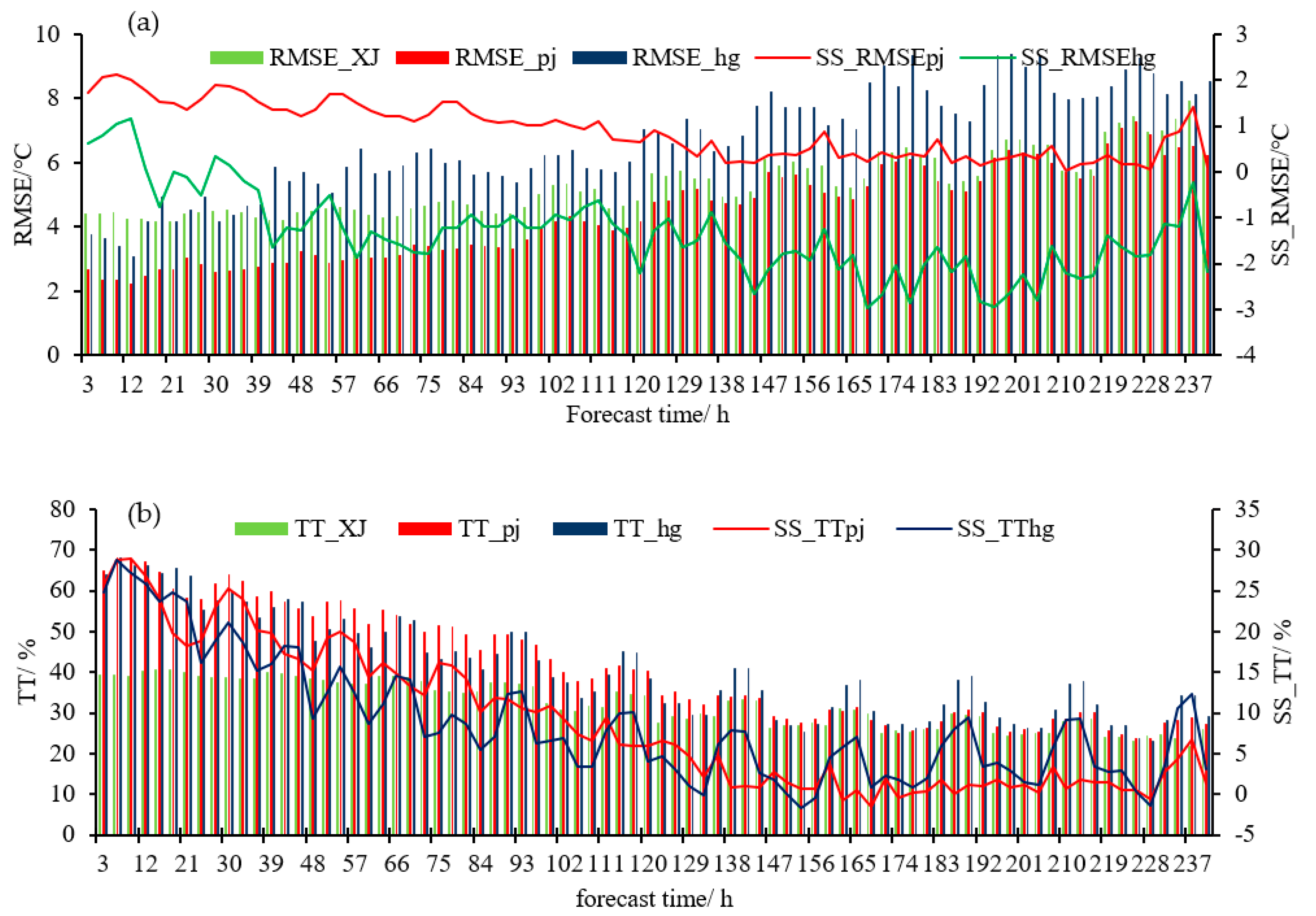
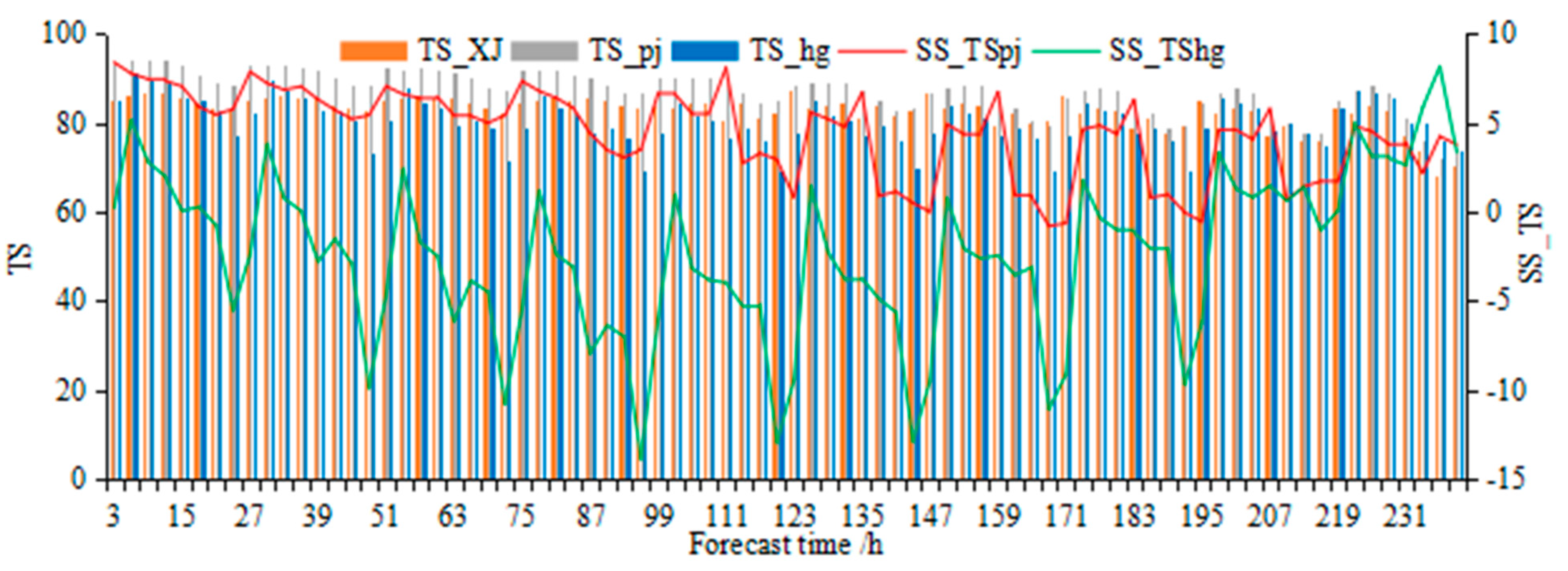
3.1.1. Time Series Comparison of Temperature Forecast

Figure 2a and Table 1 show that the mean–root errors of XJ, HG, and PJ products were 5.17, 6.77, and 4.59 °C, respectively. As compared to XJ, the RMSEs of HG and PJ were increased by 1.6 °C and decreased by 0.58 °C, respectively, and the correction effect was better within 72 h. The RMSE of PJ forecast products was lower than that of XJ, and the correction technique values were positive, as compared to HG. The forecast period was shorter than 33 h at 1400–1700 (Beijing time), and the RMSEs of HG and PJ were 0.6 and 1.93 °C lower than XJ, respectively. The forecast period was shorter than 81 h at 1100, 1400, 1700, 2000, and 2300 (Beijing time), and the RMSEs of the HG and PJ forecast products increased by 0.23 °C and decreased by 1.74 °C, as compared to XJ, respectively.
Figure 2b and Table 1 show that the average accuracy of temperature forecast for XJ, HG, and PJ were 35.52, 41.65, and 41.83%, respectively. As compared to XJ, the temperature forecast accuracy of HG and PJ increased by 9.13 and 9.30%, respectively; the positive prediction accuracy correction techniques values of HG and PJ were within 129 and 165 h, respectively, and the temperature forecast accuracy of HG and PJ increased by 22.68 and 25.17%, respectively; the accuracy correction effect on PJ was better than that of HG.

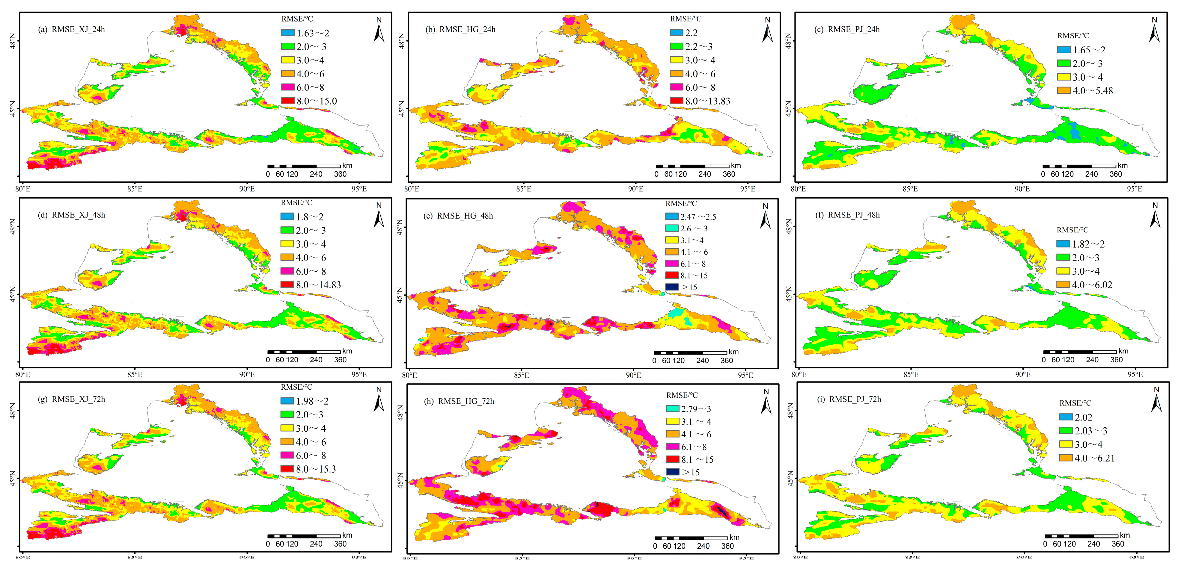
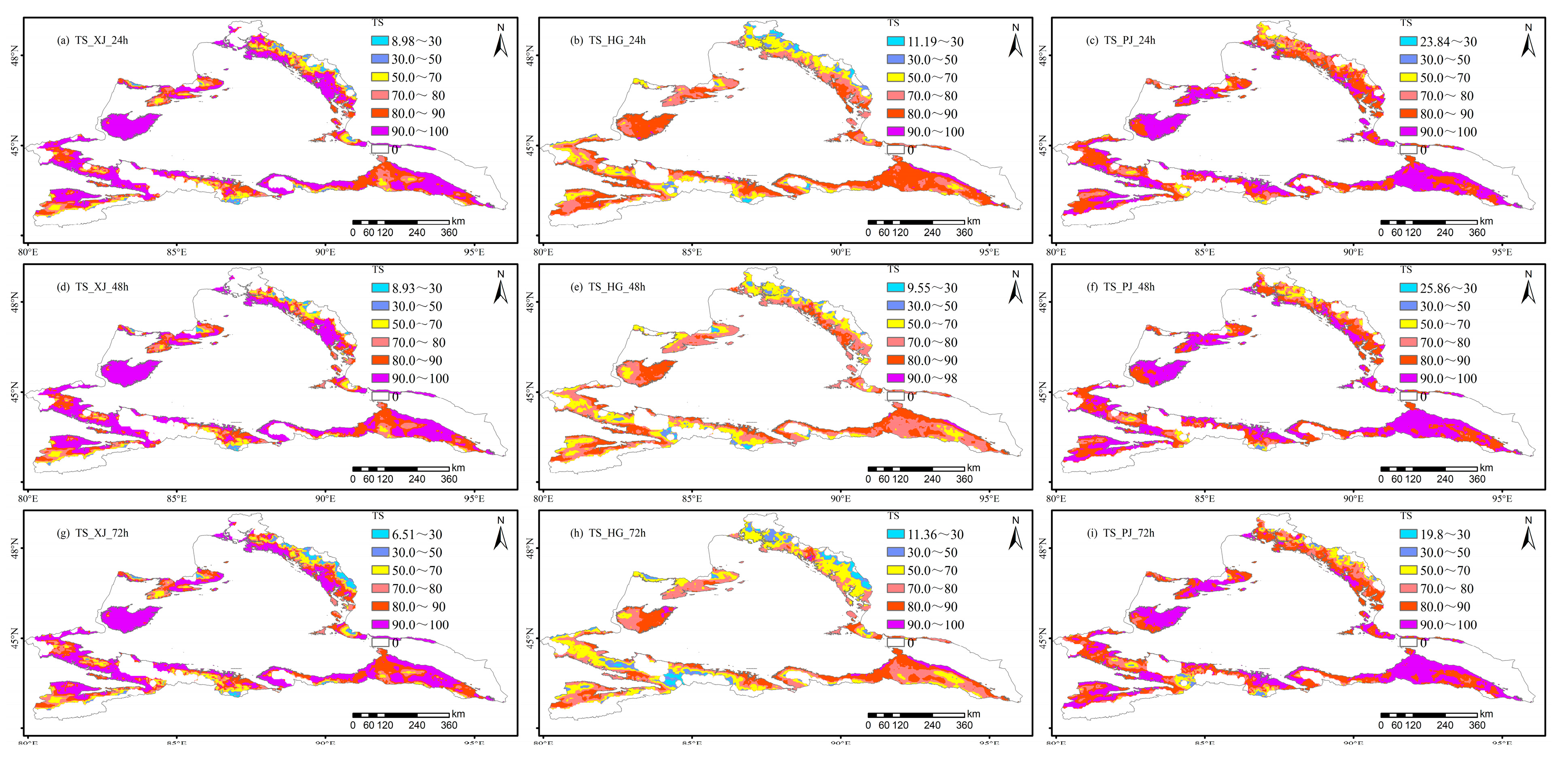
3.1.2. Spatial Distribution Comparison of Temperature Forecast

Table 1 and Figure 3 show the temperature prediction accuracy of XJ, HG, and PJ in the 24 h forecast period as 40.15, 55.36, and 58.04%, respectively, with PJ having the highest prediction accuracy. After 72 h, the temperature forecast accuracy of the 3 products was below 50%. Figure 3 shows the RMSE distributions of the temperature forecasts for XJ, HG, and PJ, over 24, 48, and 72 h.
As shown in Table 1, as compared to the forecast product (XJ), there were 2496, 1536, and 1219 grid points where the RMSE correction technique of HG was positive in the 24, 48, and 72 h periods, which accounted for 33.9, 20.8, and 16.5% of the temperature forecasts in northern Xinjiang. Meanwhile, there were 5592, 5068, and 4747 grid points where the RMSE correction techniques of PJ forecast products were positive during the 24, 48, and 72 h forecast periods, accounting for 75.9, 68.8, and 64.4% of the temperature forecasts in northern Xinjiang. As compared to HG, the PJ forecast product correction techniques had evident advantages.
Figure 3 shows a total of 5592 grid points where the RMSE correction technique value of PJ in the future 24 h temperature forecast has a positive effect, 748 grid points where the RMSE correction technique value exceeded 3 °C, and 220 grid points where the RMSE correction technique value exceeded 5 °C, accounting for 75.9, 10.1, and 3.0% of the mountainous areas in northern Xinjiang, respectively. The grid points with the positive effect on the RMSE correction were distributed in most of the mountainous areas of northern Xinjiang. The grid points with the correction effect exceeding 5 °C were distributed in the areas with elevations above 3000 m in the Kharketau Mountain and 2000 m in the source region of the Burjin River in northern Altai.

3.2. Daily Maximum Temperature Test

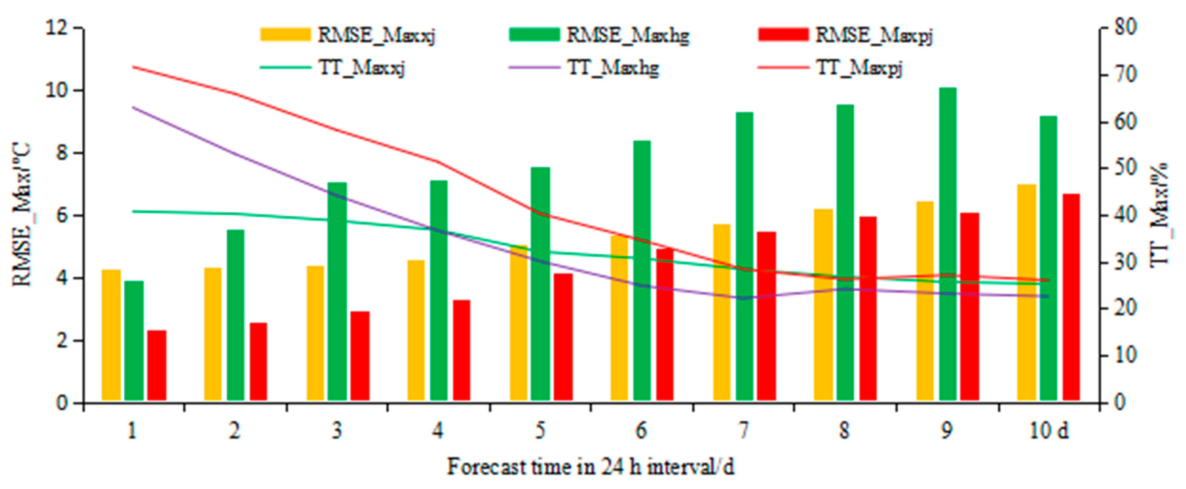
3.2.1. Time Series Comparison of Daily Maximum Temperature Forecast

Figure 4 and Table 2 show the average RMSEs of the daily maximum temperature forecast of XJ, HG, and PJ in the following 1–10 days as 5.11, 7.85, and 4.61 °C, respectively. As compared to the guide forecast product (XJ), HG increased by 2.74 °C, exhibiting a negative effect overall, where only the correction technique value in the prediction of 1 day was positive; PJ decreased by 0.50 °C, on average, whereas the correction technique values for the 1–10 days in the future were all positive. The RMSEs of the daily maximum temperature forecast of PJ in the following 1, 2, and 3 days were 2.26, 2.54, and 2.87 °C, respectively, as compared to XJ, and the RMSEs were reduced by 1.48, 1.29, and 1.1 °C, respectively.
Figure 4 and Table 2 show the forecast accuracy of the daily maximum temperature of XJ, HG, and PJ in during 1–10 days as 32.77, 35.00, and 43.7%, respectively.
Figure 4 shows that, as compared to the guide forecast product (XJ), the accuracies of HG and PJ were increased by 2.23 and 10.96%, respectively. The correction technique values were both positive, and PJ was higher. The forecast accuracies of the daily maximum temperature of PJ for the following 1, 2, and 3 days were 71.61, 65.88, and 58.12%, respectively, and increased to be 29.19, 24.25, and 18.04% higher than XJ, respectively. The accuracy correction technique of the PJ daily maximum temperature forecasts in the mountainous areas of northern Xinjiang was obviously superior to that of HG.

3.2.2. Spatial Distribution Comparison of Daily Maximum Temperature Forecast

Figure 5 shows that there were 3056, 1736, and 992 grid points where the RMSE correction technique of HG, the daily maximum temperature forecast for the following 1, 2, and 3 days, had positive effects, accounting for 47.6, 23.6, and 13.5% of the mountainous areas in northern Xinjiang. There were 6164, 5430, and 4920 grid points where the RMSE correction technique value of the daily PJ maximum temperature forecast for the following 1, 2, and 3 days had positive effects, accounting for 83.6, 73.7, and 66.7% of the mountainous areas in northern Xinjiang. As compared to HG, the areas where the RMSE correction technique values of the daily PJ maximum temperature forecast for the following 1, 2, and 3 days were positively increased by 42.0, 48.0, and 47.9%, respectively, indicating that the correction technique value had evident advantages in the spatial area.
Figure 5 shows there were 5322, 1505, and 603 grid points with RMSE correction values for the daily maximum temperature forecasts of PJ for the following day exceeding 0, 3, and 5 °C, respectively, accounting for 72.2, 20.4, and 8.2%, respectively, of the mountainous areas in northern Xinjiang. The grid points with a positive effect on the RMSE correction technique value of the daily maximum PJ temperature forecast were distributed in most of the mountainous areas of northern Xinjiang, while the areas with a negative effect on the correction technique values were located at 1300–1500 m south of Mulei in the eastern Changji Prefecture. The grid points where the PJ correction effect exceeded 5 °C were distributed in the areas with elevations above 3000 m at Kharketau Mountain and 2000 m in the source region of the Burjin River in northern Altai.

3.3. Prediction and Test of Temperature Rise

From 23 to 30 April 2021, 7371 grid points for the daily maximum temperature average rise reached 25.63 °C in the mountainous area of northern Xinjiang, among which the single-grid maximum temperature rise was 32.96 °C. A total of 559 grid points had a temperature rise of more than 30 °C, and 3894 grid points had a temperature rise of more than 25 °C but less than or equal to 30 °C. Finally, 2388 grid points had a temperature rise of more than 20 °C but less than or equal to 25 °C. The continuous temperature rise period was selected for the daily temperature-rise amplitude forecast test.

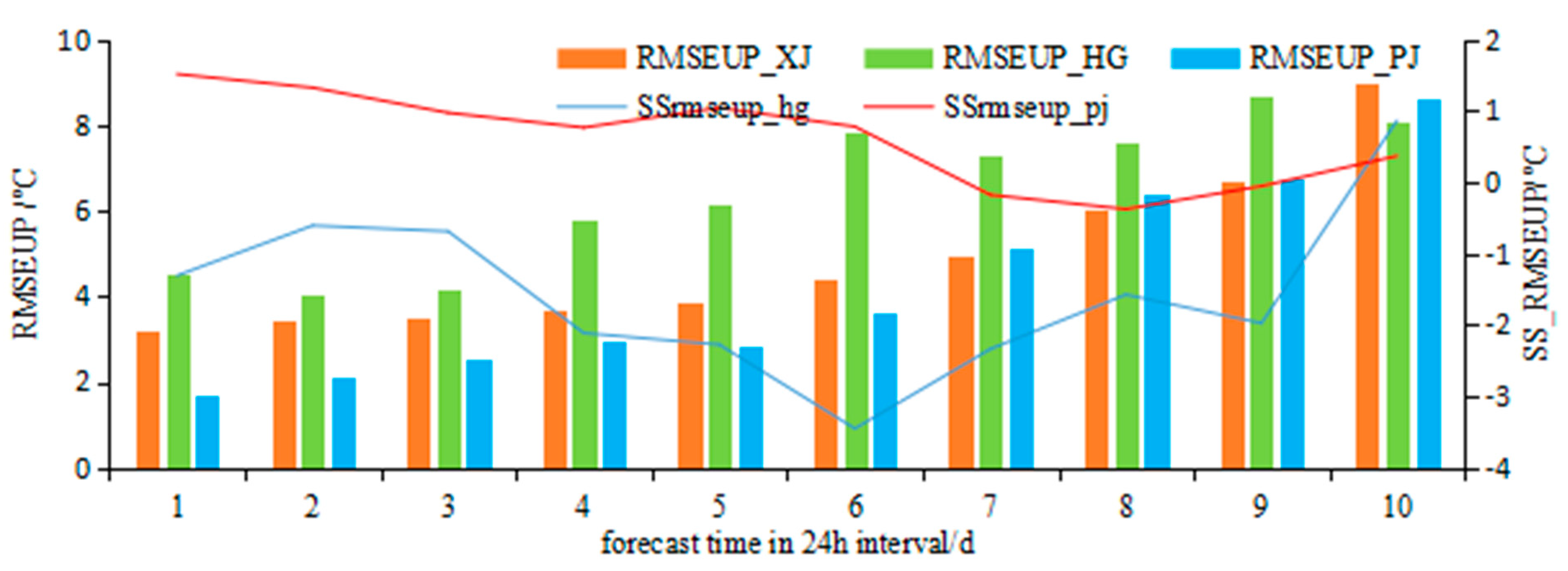
3.3.1. Forecast Period Series Comparison of Daily Temperature-Rise Amplitude

Figure 6 and Table 3 show the average RMSEs for the forecast daily temperature-rise amplitude of XJ, HG, and PJ, for the following 1–10 days, as 4.87, 6.41, and 4.25 °C, respectively. As compared to XJ, the RMSE of HG increased by 1.54 °C, while that of PJ decreased by 0.62 °C. As shown in Figure 6, as compared to the guidance product (XJ), the RMSEs of the daily temperature-rise amplitude forecast of HG for the following 1, 2, and 3 days increased by 1.32, 0.61, and 0.69 °C, respectively, and PJ was reduced by 1.50, 1.31, and 0.97 °C, respectively. The RMSEs of the daily temperature-rise amplitude forecast of the PJ for the following 1, 2, and 3 days, in the mountainous area of northern Xinjiang, were 1.69, 2.10, and 2.53 °C, respectively, and the forecast had significantly improved.

3.3.2. Spatial Distribution Comparison of Temperature-Rise Amplitude Forecast

Figure 7 and Table 3 show that as compared to XJ, there were 2768, 2875, and 2762 grid points where the RMSE correction techniques of the HG daily temperature-rise amplitude forecast for the following 1, 2, and 3 days were positive, accounting for 37.6, 39.0, and 37.5% of the mountainous areas in northern Xinjiang, respectively. Furthermore, there were 5322, 5108, and 4545 grid points with positive correction technique values of the PJ forecast product for the following 1, 2, and 3 d, accounting for 72.2, 69.3, and 61.7% of the mountainous areas in northern Xinjiang, respectively. As compared to the prediction results of HG, the number of grid points with a positive effect increased by 34.6, 30.3, and 24.2%, respectively, and the positive effect areas of PJ were significantly larger than HG.
Figure 7 shows that there were 5322, 1505, and 603 grid points with the RMSE correction techniques of the PJ daily temperature-rise amplitude forecast in the following day that exceeded 0, 3, and 5 °C, respectively, accounting for 72.2, 20.4, and 8.2%, respectively, of the mountainous areas in northern Xinjiang. Positive results were found in most of the mountainous areas in northern Xinjiang, while the correction techniques of Yili Zhaosu at an altitude of 1500–2000 m and some areas in the south of Urumqi showed negative results.

3.4. Snowmelt Temperature Tests

3.4.1. Time Series Comparison of Snowmelt Temperature

From March to May, spring 2021, the average snowmelt temperature forecast accuracies of XJ, HG, and PJ were 79.36, 74.10, and 81.99%, respectively. As compared to the guidance product (XJ), the forecast accuracy of HG decreased by 5.4%, while the PJ scheme increased by 2.45% (Figure 8 and Table 4). For a total of 80 forecast periods during the 10-day forecast period, the positive correction technique values of HG were accurate 13 and 77 times, respectively, and the correction technique value of PJ was relatively high. At 02:00, 11:00, 14:00, and 17:00 (Beijing time), the correction technique values of HG were higher than those of XJ. The average accuracy of the snowmelt temperature forecast of XJ and HG at these times was 82.16 and 84.36%, respectively.
At 02:00, 11:00, 14:00, and 17:00 (Beijing time), the correction technique values of HG were relatively high. The average accuracies of the snowmelt temperature forecast of XJ and HG at these times were 82.16 and 84.36%, respectively. At 11:00, 14:00, 17:00, and 23:00 (Beijing time), the correction technique of PJ was relatively high, and the prediction accuracies of the snowmelt temperature of XJ and PJ at these times were 84.59 and 91.60%, respectively.

3.4.2. Spatial Distribution Comparison of Snowmelt Temperature

The number of correct snowmelt grid points in CLDAS, XJ, HG, and PJ were 7324, 6609, 6641, and 6598, respectively.
Figure 9 and Table 4 show that, as compared to the original prediction (XJ), the average correction technique values of the PJ algorithm at 24, 48, and 72 h were 3.29, 3.11, and 2.42, respectively, and the positive correction technique values had 3109, 3115, and 3194 grid points, respectively. The average correction technique values of the HG algorithm at 24, 48, and 72 h were −9.8, −12.28, and −14.77, respectively, among which there were 1475, 1054, and 980 positive correction grid points, respectively.
At 24 h, the positive correction technique value grid points of the PJ algorithm were concentrated in the areas of the Yili Prefecture, 1500–2000 m above sea level; the Irenhabirgaa and Borokonu mountains at 2000–3500 m above sea level; and 3000 m above sea level, for the central Tianshan reaches east to Igo, except for the Tomulti Peak and the North Tower Mountain northward 1500 m above the Altai Mountains, as well as from the northwest of Tachen to the area of Hobuxell. The correction technique values greater than 5 had 2180 grid points in the concentrated areas, which were located in the Borokonu Mountain, Green River, and Bukser region.

3.5. Daily Snowmelt Duration Tests

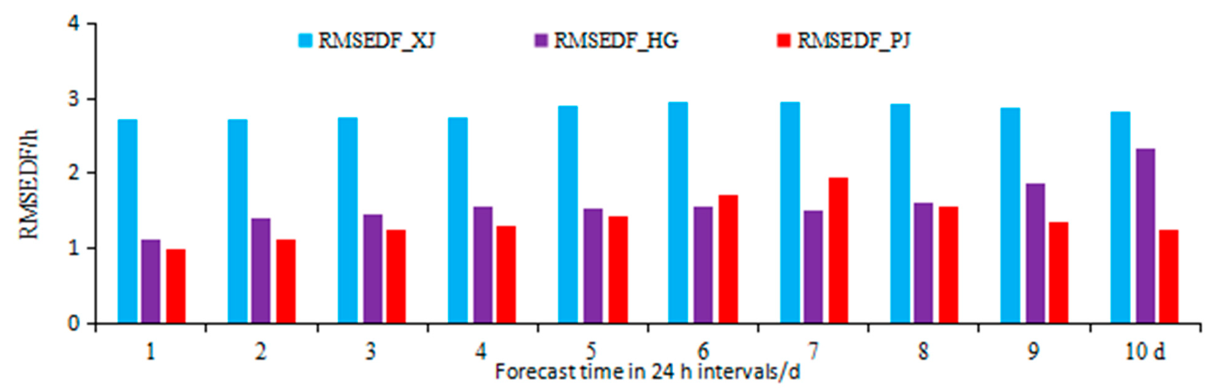
3.5.1. Time Series Comparison of Snowmelt Duration

Figure 10 and Table 5 show the RMSEs of the XJ, HG, and PJ snowmelt duration forecast for the following 1–10 days as 2.22, 1.4, and 1.29 h, respectively. As compared to XJ, the mean square errors of HG and PJ daily snowmelt durations were decreased by 0.81 and 0.93 h, respectively. Figure 10 shows that the RMSEs of HG forecast products for the following 1, 2, and 3 days were 0.72, 0.93, and 1.03 h, respectively, which were reduced by 1.18, 0.98, and 0.9 h, relative to XJ. The RMSEs of the PJ prediction products for the following 1, 2, and 3 days were 0.66, 0.80, and 0.92 h, respectively, which were reduced by 1.24, 1.11, and 1.01 h, relative to XJ, and 0.06 h, 0.13 h, and 0.11 h, relative to HG, respectively. Thus, the RMSE correction technique of the PJ snowmelt duration in the mountainous area of northern Xinjiang was superior.

3.5.2. Spatial Distribution Comparison of Snowmelt Duration Forecast

Figure 11 and Table 5 show that, as compared to XJ forecast products, there were 4373, 3964, and 3778 grid points where the RMSE correction technique values of HG daily snowmelt duration forecast products were positive in the following 1, 2, and 3 d, accounting for 59.3, 53.8, and 51.3% of the northern mountainous areas of Xinjiang, respectively. As compared to XJ, 4445, 4143, and 3952 grid points with positive correction techniques of PJ forecast products for the following 1, 2, and 3 days accounted for 60.3, 56.2, and 53.6% of the mountainous areas in northern Xinjiang, respectively. As compared to HG, the areas of the PJ forecast products’ positive correction technique values in the following 1, 2, and 3 days increased by 1.0, 2.4, and 2.4%, respectively.
Figure 11 shows that the grid with the RMSE correction technique of the PJ daily snowmelt duration forecast for the following day covered all study areas, among which there were 334 grid points with the correction technique exceeding 5 h, concentrated in the areas above 3000 m altitude in the Yili region, the upper Burtin River in the northern Altai Mountains, and partial areas that were 3000 m above sea level at the eastern end of Mount Borokonu.

4. Conclusions

4.1. Algorithm Test Results

Through the afore-described comparative test analysis, we obtained the following conclusions:
(1) Temperature forecast test by forecast period: In the 10-day, 3 h interval forecast, as compared to the guidance forecast product (XJ), the RMSEs of the HG and PJ temperature forecast products increased by 1.6 °C and decreased by 0.58 °C, respectively, and the temperature forecast accuracy increased by 9.13 and 9.30%, respectively. The RMSEs and the prediction accuracy of the temperature forecast, as well as the effects on the PJ intelligent grid temperature forecast correction technique, were significantly better than those of HG.
(2) Test of daily maximum temperature forecast: In the 10-day forecast, as compared to the guidance forecast product (XJ), the RMSE of the daily maximum temperature of the HG and PJ temperature forecast products increased by 2.74 °C and decreased by 0.5 °C, respectively, and the temperature forecast accuracy increased by 2.23 and 10.96%, respectively. The accuracy correction technique of the PJ daily maximum temperature forecast in the mountainous areas of northern Xinjiang evidently outperformed HG.
(3) Daily temperature-rise prediction test: In the 10-day forecast, as compared to the guidance forecast product (XJ), the RMSE of the daily temperature-rise amplitude of HG increased by 1.55 °C, and the correction technique exhibited a negative effect overall, while PJ decreased by 0.62 °C, which exhibited a positive effect overall.
(4) Test of snowmelt temperature forecast: In the 10-day, 3 h interval forecast, as compared to the guidance forecast product (XJ), the accuracy of the snowmelt temperature forecast of HG and PJ decreased by 5.4% and increased by 2.45%, respectively. Among the 80 forecasts within 10 days, the positive correction techniques of HG and PJ were accurate 13 and 77 times, respectively, and the accuracy correction techniques of PJ were relatively high.
(5) Test of snowmelt daily duration forecast: In the 10-day forecast, as compared to the guidance product (XJ), the mean square error of the HG and PJ snowmelt duration forecast decreased by 0.81 h and 0.93 h, respectively. The effect on the PJ correction technique was superior to that of HG.
According to the comprehensive test of the time series and spatial distribution, the original forecast products corrected by the average filter algorithm were superior to those corrected by the dynamic unary regression algorithm and the original forecast products.

4.2. Limitations and Novelty

Herein, SCMOC was selected as the original forecast product and used to design two correction algorithms. The dynamic linear regression and the average filter correction algorithms were selected according to numerous experiments using the meteorological observation station forecasts. Only the average filtering algorithm had a strong adaptability, which effectively reduced the prediction error of the grid prediction products. Though other correction algorithms exist, all must forecast and test the temperature-rise process of snowmelt in mountainous areas to determine their suitability.
The dynamic linear regression algorithm dynamically updated the coefficients in the equation. The average filtering algorithm dynamically improved the error. The different improvement points of the two algorithms were based on the Kalman filter correction theory and used the latest live data to continuously update the forecast data [29]. In order to predict the temperature-rise process more accurately, we designed four innovative temperature forecast methods, including daily maximum temperature, daily temperature-rise range, snowmelt temperature, and daily snowmelt duration. Subsequently, the algorithm could be applied to test other areas and combined with the advantages of other algorithms to design a comprehensive approach. Laypeople need more accurate temperature forecast values; thus, the algorithm in this paper can provide a technical reference for independent meteorological/commercial organizations.
We studied an intelligent grid temperature prediction technology for snowmelt warming in mountainous areas during spring. These efforts to obtain optimal grid point temperature forecasting products during snowmelt in mountainous areas contributes to the growing technical support for predicting snowmelt flood periods and estimating flood-peak discharge. To monitor and forecast the temperature-rise change process of each grid in mountainous areas during snowmelt seasons, we provided a scientific assessment of the snowmelt time, speed, and snowmelt quantity as well as a quantitative analysis of snowmelt flood changes in the river basin, and we provided a scientific basis for guiding agricultural production layout, water resource management, and accurate disaster prevention and avoidance.

4.3. Discussion

This paper discusses the problem of the temperature forecast during the snowmelt period. However, there are many factors affecting snowmelt, such as evapotranspiration [41], the amount of sunshine, the structure of the snow, the surface coverage of the snow cover [42] and precipitation [43,44], etc., which have an effect on snowmelt, considering these factors, more aspects should be considered in the later stage of this study.

Author Contributions

Conceptualization, Z.Z. and M.W.; Methodology, Z.Z.; Software, Z.Z.; Validation, W.Z. and A.M.; Formal analysis, Z.Z.; Investigation, Z.Z., W.Z. and D.A.; Resources, W.M.; Data curation, M.W.; Writing—original draft, Z.Z.; Writing—review and editing, W.M. and M.W.; Visualization, C.J.; Supervision, M.W. and C.J.; Funding acquisition, W.M. All authors have read and agreed to the published version of the manuscript.

Funding

This research was funded by the National Key Research and Development Program of China (2019YFC1510501), the National Natural Science Foundation of China (NSFC) (41975146), and the Natural Science Foundation of Xinjiang Uygur Autonomous Region (PT2323).

Data Availability Statement

Supplementary data to this article can be found online at http://data.cma.cn/ (accessed on 1 June 2022).

Conflicts of Interest

The authors declare no conflict of interest.

References

  1. Zhong, X.Y.; Zhang, T.J.; Su, H.; Xiao, X.X.; Wang, S.F.; Hu, Y.T.; Wang, H.J.; Zheng, L.; Zhang, W.; Xu, M.; et al. Impacts of landscape and climatic factors on snow cover in the Altai Mountains, China. Adv. Clim. Chang. Res. 2021, 12, 95–107. [Google Scholar] [CrossRef]
  2. Zhang, H.; Wang, F.T.; Zhou, P. Changes in climate extremes in a typical glacierized region in central Eastern Tianshan Mountains and their relationship with observed glacier mass balance. Adv. Clim. Chang. Res. 2022, 13, 909–922. [Google Scholar] [CrossRef]
  3. Zhou, Y.; Li, G.Y.; Jin, H.J.; Marchenko, S.S.; Ma, W.; Du, Q.S.; Li, J.M.; Chen, D. Viscous creep of ice-rich permafrost debris in a recently uncovered proglacial area in the Tianshan Mountains, China. Adv. Clim. Chang. Res. 2022, 13, 540–553. [Google Scholar] [CrossRef]
  4. Li, J.; Zhang, Y.T.; Zhang, Y.Y. Impact of seasonal snowmelt on snowpack at woodland, grassland and bare land in North Slope of Tian Mountain. J. Irrig. Drain. 2021, 40, 106–114. [Google Scholar] [CrossRef]
  5. Xiang, Y.Y.; Wang, Z.Z.; Zhang, W.; Chen, Y.Y. Study of snowmelt runoff simulation in arid regions: Progress and prospect. J. Glaciol. Geocryol. 2017, 39, 892–901. [Google Scholar]
  6. Wang, X.Q.; Lu, X.Y.; Ma, Y.; Wang, X. Study on snow disaster assessment method and snow disaster regionalization in Xinjiang. J. Glaciol. Geocryol. 2019, 41, 836–844. [Google Scholar] [CrossRef]
  7. Jeelani, G.; Feddema, J.J.; Van der Veen, C.J.; Stearns, L. Role of snow and glacier melt in controlling river hydrology in Liddar watershed (western Himalaya) under current and future climate. Water Resour. Res. 2012, 48, W12508. [Google Scholar] [CrossRef]
  8. Cho, E.; Jacobs, J.M. Extreme value snow water equivalent and snowmelt for infrastructure design over the contiguous United States. Water Resour. Res. 2020, 56, e2020WR028126. [Google Scholar] [CrossRef]
  9. Sadro, S.; Sickman, J.O.; Melack, J.M.; Skeen, K. Effects of climate variability on snowmelt and implications for organic matter in a high-elevation lake. Water Resour. Res. 2018, 54, 4563–4578. [Google Scholar] [CrossRef]
  10. Wang, H.; Wang, M.X.; Wang, S.L.; Yu, X.J. Spatial-temporal variation characteristics of snow cover duration in Xinjiang from 1961 to 2017 and their relationship with meteorological factors. J. Glaciol. Geocryol. 2021, 43, 61–69. [Google Scholar] [CrossRef]
  11. Hanati, G.L.M.R.; Zhang, Y.; Su, L.D.; Hu, K.K. Response of water and heat of seasonal frozen soil to snow melting and air temperature. Arid Land Geogr. 2021, 44, 889–896. [Google Scholar] [CrossRef]
  12. Mao, W.Y.; Fan, J.; Shen, Y.P.; Yang, Q.; Gao, Q.Z.; Wang, G.Y.; Wang, S.D.; Wu, S.F. Variations of extreme flood of the rivers in Xinjiang region and some typical watersheds from Tianshan Mountains and their response to climate change in recent 50 years. J. Glaciol. Geocryol. 2012, 34, 1037–1046. [Google Scholar] [CrossRef]
  13. Laudon, H.; Seibert, J.; Köhler, S.; Bishop, K. Hydrological flow paths during snowmelt: Congruence between hydrometric measurements and oxygen 18 in meltwater, soil water, and runoff. Water Resour. Res. 2004, 40, W03102. [Google Scholar] [CrossRef]
  14. Zhang, J.L.; Luo, J.; Wang, R.M. Combined analysis of the spatiotemporal variations in snowmelt (ice) flood frequency in Xinjiang over 20 years and atmospheric circulation patterns. Arid Zone Res. 2021, 38, 339–350. [Google Scholar] [CrossRef]
  15. Tian, H.; Yang, X.D.; Zhang, G.P.; Zhao, L.N.; Wang, Z.; Zhao, L.Q. The possible weather causes for snowmelt flooding in Xinjiang in Mid-March 2009. Meteorol. Mon. 2011, 37, 590–598. [Google Scholar] [CrossRef]
  16. Qin, Y.; Zhao, Q.D.; Liu, Y.Q.; Ding, J.L. Response of snow hydrological processes to climate change in the Hutubi river basin on the North Slope of Tian Shan mountains. J. Soil Water Conserv. 2021, 35, 190–199. [Google Scholar] [CrossRef]
  17. Zhou, G.; Cui, M.Y.; Li, Z.; Zhang, S.Q. Dynamic evaluation of the risk of the spring snowmelt flood in Xinjiang. Arid Zone Res. 2021, 38, 950–960. [Google Scholar] [CrossRef]
  18. Mercado-Bettín, D.; Clayer, F.; Shikhani, M.; Moore, T.N.; Frías, M.D.; Blake, L.J.; Sample, J.; Lturbide, M.; Herrera, S.; French, A.S.; et al. Forecasting water temperature in lakes and reservoirs using seasonal climate prediction. Water Res. 2021, 201, 117286. [Google Scholar] [CrossRef]
  19. Yan, J.; Liao, G.Y.; Gebremichael, M.; Shedd, R.; Vallee, D.R. Characterizing the uncertainty in river stage forecasts conditional on point forecast values. Water Resour. Res. 2012, 48, W12509. [Google Scholar] [CrossRef]
  20. Kim, Y.; Sartelet, K.; Raut, J.C.; Chazette, P. Evaluation of the Weather Research and Forecast/Urban Model Over Greater Paris. Bound. Layer Meteorol. 2013, 149, 105–132. [Google Scholar] [CrossRef]
  21. Battisti, A.; Acevedo, O.C.; Costa, F.D. Evaluation of Nocturnal Temperature Forecasts Provided by the Weather Research and Forecast Model for Different Stability Regimes and Terrain Characteristics. Bound. Layer Meteorol. 2017, 162, 523–546. [Google Scholar] [CrossRef]
  22. Liu, L.; Xu, Y.P.; Pan, S.L.; Bai, Z.X. Potential application of hydrological ensemble prediction in forecasting floods and its components over the Yarlung Zangbo River basin, China, Hydrol. Earth System Science Data 2019, 23, 3335–3352. [Google Scholar] [CrossRef]
  23. Deng, Q.; Yang, J.; Zhang, L.; Sun, Z.; Sun, G.; Chen, Q.; Dou, F. Analysis of Seasonal Driving Factors and Inversion Model Optimization of Soil Moisture in the Qinghai Tibet Plateau Based on Machine Learning. Water 2023, 15, 2859. [Google Scholar] [CrossRef]
  24. Nayak, M.A.; Herman, J.D.; Steinschneider, S. Balancing flood risk and water supply in California: Policy search integrating short-term forecast ensembles with conjunctive use. Water Resour. Res. 2018, 54, 7557–7576. [Google Scholar] [CrossRef]
  25. Jiang, Z.; Xu, T.; Mariethoz, G. Numerical investigation on the implications of spring temperature and discharge rate with respect to the geothermal background in a fault zone. Hydrogeol. J. 2018, 26, 2121–2132. [Google Scholar] [CrossRef]
  26. Krainer, K.; Winkler, G.; Pernreiter, S.; Wagner, T. Unusual catchment runoff in a high alpine karst environment influenced by a complex geological setting (Northern Calcareous Alps, Tyrol, Austria). Hydrogeol. J. 2021, 29, 2837–2852. [Google Scholar] [CrossRef]
  27. Hegdahl, T.J.; Engeland, K.; Steinsland, I.; Tallaksen, L.M. Streamflow forecast sensitivity to air temperature forecast calibration for 139 Norwegian catchments. Hydrol. Earth Syst. Sci. 2019, 23, 723–739. [Google Scholar] [CrossRef]
  28. Regonda, S.K.; Rajagopalan, B.; Clark, M.; Zagona, E. A multimodel ensemble forecast framework: Application to spring seasonal flows in the Gunnison River Basin. Water Resour. Res. 2006, 42, W09404. [Google Scholar] [CrossRef]
  29. Zhang, Z.L.; Mao, W.Y.; Zhang, S.Q.; Wang, M.Q.; Tang, Y.; Mushajiang, A.D.T.L.d; Yusupu, T.R.G. Correction and verification for grid refined forecast of temperature and frost in spring in Northern Xinjiang. Meteorol. Mon. 2022, 48, 1460–1474. [Google Scholar] [CrossRef]
  30. Fan, H.; Liu, Y.; Li, Y.; Liu, Y.; Duan, J.; Li, L.; Huo, Z.Y. A deep learning method for predicting lower troposphere temperature using surface reanalysis. Atmos. Res. 2023, 283, 106542. [Google Scholar] [CrossRef]
  31. Zhang, W.; Jiang, Y.; Dong, J.; Song, X.J.; Pang, R.B.; Guoan, B.Y.; Yu, H. A deep learning method for real-time bias correction of wind field forecasts in the Western North Pacific. Atmos. Res. 2023, 284, 106586. [Google Scholar] [CrossRef]
  32. Dai, Y.; He, N.; Fu, Z.Y. Beijing intelligent grid temperature objective prediction method (BJTM) and verification of forecast result. J. Arid Meteorol. 2019, 37, 339–344. [Google Scholar] [CrossRef]
  33. Hao, C.; Zhang, Y.X.; Wang, Z.W.; Fu, Z.Y. Application of analog ensemble rectifying method in objective temperature prediction. Meteorol. Mon. 2019, 45, 1085–1092. [Google Scholar] [CrossRef]
  34. Hou, Z.L.; Li, J.P.; Wang, L.; Zhang, Y.Z.; Liu, T. Improving the forecast accuracy of ECMWF 2-m air temperature using a historical dataset. Atmos. Res. 2022, 273, 106177. [Google Scholar] [CrossRef]
  35. Wei, Q.; Dai, K.; Lin, J.; Zhao, R.X. Evaluation on the 2016–2018 fine gridded precipitation and temperature forecasting. Meteorol. Mon. 2020, 46, 1272–1285. [Google Scholar] [CrossRef]
  36. Wang, F.J.; Zhao, C.H.; Ma, Y.; Xia, Z.Y. Prediction effectiveness verification of ECMWF Fine grid model for air temperature in Qingdao region. Meteorol. Sci. Technol. 2018, 46, 112–120. [Google Scholar] [CrossRef]
  37. Li, G.; Yang, X.Z.; Liu, Y.H.; Chen, Z.H.; Yu, Q.; Wu, C.H. Forecast of maximum temperature based on refined guidance SCMOC data in Guizhou Province. J. Arid Meteorol. 2020, 38, 457–464. Available online: http://www.ghqx.org.cn/CN/Y2020/V38/I03/457 (accessed on 28 June 2020).
  38. Liu, X.W.; Duan, B.L.; Huang, W.B.; Duan, M.J.; Li, R.; Di, X.H.; Wei, S.J. Application of objective prediction method based on wavelet analysis in intelligent grid high and low temperature prediction. Trans. Atmos. Sci. 2020, 43, 577–584. [Google Scholar] [CrossRef]
  39. Meteorological Center, C.M.A. CLDAS2.0 Dataset Description. 19 January 2017. Available online: http://data.cma.cn/data/detail/dataCode/NAFP_CLDAS2.0_NRT.html (accessed on 1 June 2022).
  40. Liu, Y.; Shi, C.X.; Wang, H.J.; Han, S. Applicability assessment of CLDAS temperature data in China. Trans. Atmos. Sci. 2021, 44, 540–548. [Google Scholar] [CrossRef]
  41. Gan, G.J.; Wu, J.L.; Hori, M.; Fan, X.W.; Liu, Y.W. Attribution of decadal runoff changes by considering remotely sensed snow/ice melt and actual evapotranspiration in two contrasting watersheds in the Tienshan Mountains. J. Hydrol. 2022, 610, 127810. [Google Scholar] [CrossRef]
  42. Hidalgo-Hidalgo, J.-D.; Collados-Lara, A.-J.; Pulido-Velazquez, D.; Rueda, F.J.; Pardo-Igúzquiza, E. Analysis of the Potential Impact of Climate Change on Climatic Droughts, Snow Dynamics, and the Correlation between Them. Water 2022, 14, 1081. [Google Scholar] [CrossRef]
  43. Xiong, W.; Tang, G.; Wang, T.; Ma, Z.; Wan, W. Evaluation of IMERG and ERA5 Precipitation-Phase Partitioning on the Global Scale. Water 2022, 14, 1122. [Google Scholar] [CrossRef]
  44. Zhu, G.F.; Wang, L.; Liu, Y.W.; Bhat, M.A.; Qiu, D.D.; Zhao, K.L.; Sang, L.Y.; Lin, X.R.; Ye, L.L. Snow-melt water: An important water source for Picea crassifolia in Qilian Mountains. J. Hydrol. 2022, 613A, 128441. [Google Scholar] [CrossRef]
Figure 1. Overview map of mountainous areas in northern Xinjiang.
Water 15 03337 g001
Figure 2. Time series distribution of RMSE (a), forecast accuracy (b), and correction techniques of three temperature forecast products in the mountainous areas of northern Xinjiang.
Water 15 03337 g002
Figure 3. Spatial distribution of RMSE for 0–24, 24–48, and 48–72 h temperature forecasts (columns: XJ, HG, and PJ forecast from left to right; Rows: 0–24, 24–48, and 48–72 h from top to bottom).
Water 15 03337 g003
Figure 4. Time series distribution of RMSEs and the prediction accuracy during 1–10 days of daily maximum temperature forecasts in mountainous areas of northern Xinjiang.
Water 15 03337 g004
Figure 5. Spatial distribution of RMSEs in the following 1, 2, and 3 days, for daily maximum temperature forecasts in the mountainous areas of northern Xinjiang (columns: XJ, HG, and PJ forecast from left to right; rows: 1, 2, and 3 days from top to bottom).
Water 15 03337 g005
Figure 6. Time series distribution of RMSEs and correction technique of daily temperature-rise amplitude forecast for the following 1–10 days in mountainous areas of northern Xinjiang.
Water 15 03337 g006
Figure 7. Spatial distribution of RMSEs for daily temperature-rise amplitude forecast for the following 1, 2, and 3 days in the mountainous areas of northern Xinjiang (columns: XJ, HG, and PJ forecast from left to right; rows: 1, 2, and 3 days from top to bottom).
Water 15 03337 g007
Figure 8. Time series of snowmelt temperature forecast accuracy and correction techniques values of three kinds of forecast products in spring in mountainous areas of northern Xinjiang within the 10-day forecast period.
Water 15 03337 g008
Figure 9. Spatial distribution of snowmelt temperature forecast accuracy at 24, 48, and 72 h (columns: XJ, HG, and PJ forecast from left to right; rows: 24 h, 48 h, and 72 h forecast periods, from top to bottom, respectively).
Water 15 03337 g009
Figure 10. Daily distribution of RMSEs of daily snowmelt duration forecast for the following 1–10 days in the mountainous areas of northern Xinjiang.
Water 15 03337 g010
Figure 11. Spatial distribution of RMSEs of daily snowmelt duration forecast for the following 1, 2, and 3 days in the mountainous areas of northern Xinjiang (columns: XJ, HG, and PJ forecast from left to right; rows: 1, 2, and 3 days from top to bottom).
Water 15 03337 g011
Table 1. Test effect on root–mean–square error, temperature prediction accuracy, and the correction techniques of three prediction products. (↓: The test value is lower than the original forecast. ↑: The test value is higher than the original forecast).
Average Value of the Forecast Period0–240 hCorrection Techniques0–24 h24–48 h48–72 h72–96 h96–120 h120–240 h
RMSE_XJ/°C5.17 4.044.114.224.34.556.19
RMSE_HG/°C6.77−1.60 ↓4.375.375.95.476.668.01
RMSE_PJ/°C4.590.58 ↑2.973.183.393.544.116.21
TT_XJ/%32.52 40.1539.3738.8237.1934.5626.24
TT_HG/%41.659.13 ↑55.3647.944.9242.9138.3929.14
TT_PJ/%41.839.30 ↑58.0453.8250.146.840.327.31
Table 2. RMSE and prediction accuracy of daily maximum temperature forecasts in mountainous areas of northern Xinjiang. (↓: The test value is lower than the original forecast. ↑: The test value is higher than the original forecast).
Average Value of Forecast Period in 24 h Interval240 hCorrection Techniques1 d2 d3 d4 d5 d10 d
RMSE_Max_XJ/°C5.11 3.743.833.974.204.756.82
RMSE_Max_HG/°C7.85−2.74 ↓3.685.166.646.827.338.96
RMSE_Max_PJ/°C4.610.50 ↑2.262.542.873.234.066.68
TT_Max_XJ/%32.77 42.4741.6340.0837.7732.6625.27
TT_Max_HG/%35.002.23 ↑62.9153.0244.1136.5930.0522.52
TT_Max_PJ/%43.7310.96 ↑71.6165.8858.1251.3040.2525.97
Table 3. RMSEs for the daily temperature-rise amplitude forecast for mountainous area of northern Xinjiang. (↓: The test value is lower than the original forecast. ↑: The test value is higher than the original forecast).
Average Value of the Forecast Period in 24 h IntervalRange1–10 dCorrection Techniques1 d2 d3 d4 d5 d
RMSEUP_XJ/°C2.4–714.684.87 3.193.413.503.703.85
RMSEUP_HG/°C2.96–20.146.41−1.54 ↓4.514.024.195.816.13
RMSEUP_PJ/°C2.84–7.354.250.62 ↑1.692.102.532.942.82
Table 4. Regional and time division comparison of snowmelt temperature forecast accuracy for three kinds of forecast products. (↓: The test value is lower than the original forecast. ↑: The test value is higher than the original forecast).
Average Forecast PeriodRange240 hCorrection Techniques24 h48 h72 h96 h120 h240 h
TS_XJ0.09–99.8479.36 82.3582.6580.9482.6482.166.29
TS_HG0.26–99.0774.1−5.4 ↓71.7268.865.9363.664.6868.01
TS_PJ1.45–98.9881.992.45 ↑85.1284.7883.2283.0681.7166.75
Table 5. RMSEs in the daily snowmelt duration forecast for mountainous areas of northern Xinjiang. (↑: The test value is higher than the original forecast).
Average Value of the Forecast Period in 24 h IntervalRange1–10 dCorrection Techniques1 d2 d3 d4 d5 d10 d
RMSEDF_XJ/h0–14.622.22 1.901.911.931.972.072.04
RMSEDF_HG/h0–7.21.400.81 ↑0.720.931.031.071.031.85
RMSEDF_PJ/h0–5.681.290.93 ↑0.660.800.920.951.100.81
Disclaimer/Publisher’s Note: The statements, opinions and data contained in all publications are solely those of the individual author(s) and contributor(s) and not of MDPI and/or the editor(s). MDPI and/or the editor(s) disclaim responsibility for any injury to people or property resulting from any ideas, methods, instructions or products referred to in the content.

