Abstract
Numerical simulation of unsteady free surface flows using depth averaged equations that consider the presence of initial discontinuities has been often reported for situations dealing with dam break flow. The usual approach is to assume a sudden removal of the gate at the dam location. Additionally, in order to prevent any kind of dam risk in earthen dams, it is very interesting to include the possibility of a progressive dam breach leading to dam overtopping or dam piping so that predictive hydraulic models benefit the global analysis of the water flow. On the other hand, when considering a realistic large domain with complex topography, a fine spatial discretization is mandatory. Hence, the number of grid cells is usually very large and, therefore, it is necessary to use parallelization techniques for the calculation, with the use of Graphic Processing Units (GPU) being one of the most efficient, due to the leveraging of thousands of processors within a single device. The aim of the present work is to describe an efficient GPU-based 2D shallow water flow solver (RiverFlow2D-GPU) supplied with the formulation of internal boundary conditions to represent dynamic dam failure processes. The results obtained indicate that it is able to develop a transient flow analysis taking into account several scenarios. The efficiency of the model is proven in two complex domains, leading to >76× faster simulations compared with the traditional CPU computation.
1. Introduction
It is broadly accepted that, even though dams are hydraulic structures that can provide benefits, there exists a risk associated with their failure. When dams fail, the consequences can vary with the extent of the inundation area and the size of the population at risk, but they could be devastating. The possibility to simulate scenarios of dam breach events and the resulting floods with the help of computational tools is essential. It can help to anticipate and reduce threats due to potential dam failure and justifies the search for improved breach analysis tools considering different failure mechanisms.
Among the tools available today for analysing dam failures and their resulting outflow hydrograph, some of the best known are the National Weather Service (NWS) Dam-Break Flood Forecasting Model (DAMBRK), the NWS Simplified Dam-Break Flood Forecasting Model SMPDBK [1] and the NWS FLDWAV [2]. The focus is the prediction of the reservoir outflow hydrograph and its routing downstream the dam. The hydrograph depends on the breach characteristics and the reservoir shape and size. Concerning the numerical simulation of the downstream wave propagation given the breach hydrograph, models dealing with unsteady free surface flows using depth averaged equations that consider the presence of initial discontinuities are the most recent [3,4,5,6]. It is usual to assume a sudden dam removal but, in order to deal with earthen dams, it is very interesting to include the possibility of a progressive dam breach that can lead to dam over-topping or dam piping. In this scenario, the predictive hydraulic model offers a global analysis of the water flow in dynamic conditions including warning time as sum of the breach initiation time, breach formation time and flood wave travel [7].
It is therefore justified to devote time and effort to the development of accurate and complete advanced simulation models able to incorporate the dynamic breach formation in the context of ambitious wave propagation computations. Recent advances in this sense have led to a new generation of tools based on finite volume techniques for the 2D shallow water equations that can be used for real time flow predictions [8]. When considering a realistic large domain with complex topography, a fine spatial discretization is mandatory. Hence, the number of grid cells is usually very large and, therefore, it is necessary to use parallelization techniques for the calculation, with the use of Graphic Processing Units (GPU) being one of the most efficient due to the leveraging of thousands of processors within a single device [9]. As the computational efficiency of the numerical method used is limited by the stability restriction, a CUDA-based implementation on GPU is used. This is the core tool of the RiverFlow2D-GPU software developed by the authors and distributed by Hydronia LLC [10,11,12,13]. It is able to develop a transient flow analysis taking into account several scenarios. The main objective of the present work is to report on the enhancement of the 2D shallow water flow model RiverFlow2D-GPU by means of a dynamic internal boundary conditions that allow the simulation of the evolution of dam breach processes as well as the propagation of the subsequent overland flow waves.
The outline of the present paper is as follows: First, the governing 2D shallow water equations are recalled together with the formulation chosen to model the dam failure processes including erosion, collapse and overflow. Then, the finite volume scheme used to solve the partial difference system on unstructured triangular cells is outlined. The novel formulation of internal boundary conditions representing several dam breach processes and the strategy adopted to incorporate the presence of the dam and its failure through piping is described. Two test cases are presented to show the model performance. In the absence of good experimental data, synthetic test cases are used. First, a case to simulate a collapse that leads to the transition from piping to dambreach. Then, a representative range of data collected by the USDA is also reproduced to show the efficiency of the model complex domains, leading to >76× faster simulations compared with the traditional CPU computation.
2. Governing Equations and Computational Model
2.1. Governing Equations
The surface flow in the present work is described by means of the depth averaged 2D shallow water system of equations. They can be compactly formulated in terms of the conserved variables [14]:
where h is the water depth and and the unit discharges in x and y direction, respectively. The fluxes of mass and momentum are:
The bed slopes and friction terms are included on the source term of the system:
where bed slopes in both plane directions are:
and friction is formulated using the semi-empirical Manning law:
where n is Manning’s roughness coefficient [15].
2.2. Dambreach by Piping-Erosion Model
The novelty presented in this work is the formulation of internal boundary conditions representing several dam breach processes in combination with the 2D shallow water model. The 2D surface flow model is combined with a piping/dam breach evolution model presented in Chen et al. [16]. The cross-section of the pipe is assumed to be initially composed of a semicircular arch of radius at the top with a square of side b at the bottom. Orifice flow and open channel flow equations are chosen to model the discharge for pressurized and free surface flows through the pipe, respectively.
2.2.1. Flow Discharge through the Pipe
If the pipe is fully filled with water, the discharge through can be estimated using the following orifice equation:
where:
- is the cross-sectional area of the pipe;
- b is the width of the base of the pipe;
- is the elevation of the pipe centre line;
- is the elevation of the pipe bottom;
- is the elevation of the water surface level;
- L is the pipe length;
- is the pipe hydraulic radius;
- is the pipe wetted perimeter;
- is the Darcy–Weisbach friction factor of the pipe surface;
- is Manning’s roughness coefficient of the pipe surface;
- is a constant (Wu [17]).
On the other hand, in the case of a partially filled pipe, roof collapse or overtopping, the discharge is computed by means of a free surface flow equation:
where:
- is a dimensionless submergence correction for tailwater effects ([18]);
- is the breach side slope angle with respect to the horizontal;
- is a discharge coefficient for the rectangular part of the breach section [19];
- is a discharge coefficient for the triangular part of the breach section [19].
2.2.2. Pipe Erosion
Regarding the erosion process, a shear stress-based formula is adopted to calculate the erosion rate. As erosion takes place, the full pipe cross section is enlarged along its height and width due to the removal of materials until the collapse of the pipe roof occurs (see Figure 1). The vertical erosion of the pipe is computed using an excess detachment rate relation:
where:
- is the measured erosion coefficient at the breach;
- is the critical stress required to initiate detachment for the material;
- is the bed shear stress in the pipe surface;
- is the water density.
The horizontal erosion rate is assumed to be equal to the vertical erosion rate and, hence, the evolution can be expressed as:
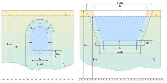
Figure 1.
Cross-section of the expansion due to piping process before the dam collapse (left) and trapezoidal breach evolution after the dam collapse (right).
2.2.3. Pipe Roof Collapse
The collapse of the pipe roof is estimated by comparing the weight of the overlying soil and the cohesion of the soil on the two sidewalls of the pipe. The failure planes are assumed to be vertical and, for the sake of simplicity, the collapse is assumed to move downstream instantaneously. The arch finally becomes unstable due to the erosion of the pipe, and the collapse of the soil mass above the arch occurs. The failure of the roof occurs if the top of the eroding pipe () reaches the top of the dam (). On the other hand, the failure also occurs if the driving force exceeds the soil resistant force (Figure 2). Hence, the model compares these two forces along the vertical direction. Once the driving force (equal to the weight of the failure part) is larger than the resistant force, the roof above the pipe will collapse:
where p is the porosity of the soil material, is the specific gravity of the soil, is the soil material density and C is the cohesion of the dam fillings. The areas , and are computed as follows:
where:
- is the dam crest width;
- ;
- ;
- is the upward dam slope angle;
- is the downward dam slope angle.
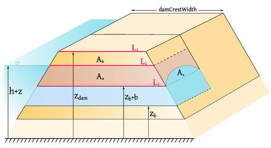
Figure 2.
Schematic diagram of the piping situation.
The collapsed pipe roof is assumed to move downstream instantaneously. After the collapse, overtopping failure dominates and the breach flow discharge and the vertical erosion can be estimated using Equations (8) and (9), respectively. The relationship between horizontal expansion and vertical undercutting is given by the change in the breach top width :
and the change in the breach bottom width is given by:
2.3. Numerical Scheme
The system of Equations (2) is mandatory to be solved numerically due to the lack of analytical solution. For that purpose, an explicit upwind finite volume scheme, based on the Riemann Solver of Roe [20], is used in this work. This numerical scheme starts from system (2) which, in compact form, can be expressed as:
where . Integrating Equation (15) in a control volume or cell, , and applying the divergence theorem to the second term:
where is the contour of the control volume and is the outgoing unit vector normal to the volume. By discretizing Equation (16) in time and space, the basis of the numerical method in finite volumes is given by:
where is the area of cell i, n is the current time level and the number of neighbouring cells is 3, because triangular cells are used in this work (as in the example in Figure 3). In addition, the fluxes E are evaluated at cell boundaries:
where is the flux value at cell , which shares a wall k, of length , with cell with flux value .
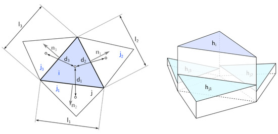
Figure 3.
Diagram of the cells in a two-dimensional case with triangular cells.
Considering the hyperbolic character of System (15), the Jacobian matrix normal to the flow direction, E, can be defined as:
The local value of the Jacobian matrix (19) can also be defined at the walls k, being :
where is the diagonal matrix whose non-zero elements are the eigenvalues of the system, , and where is the matrix containing the eigenvectors of the system, , providing this matrix with 3 eigenvalues to the 2D model. Therefore, starting from Expression (17), and using the eigenvalues and eigenvectors of the Jacobian matrix, the updating expression at cell i is obtained:
The time step is calculated dynamically throughout the simulation, following:
with , where CFL is the Courant–Friedrichs–Lewy number, which guarantees stability in the numerical scheme, and where:
The time step depends, on the one hand, on the dynamics of the problem to be solved through and, on the other hand, on the cell size chosen for the computational grid, given by . Therefore, from Equations (22) and (23), it becomes clear that increasing the refinement of the computational leads to smaller time steps, and therefore to a higher computational cost.
2.4. Dambreach Flow as Internal Boundary Condition
Expression (21) allows the variables updating scheme at each interior cell of the domain using information that comes from the neighbour cells through the cell edges. When using triangular meshes, there are three contributions to update the three conserved variables. At boundary cells, at least one of the edges does not have a neighbour cell and boundary conditions are necessary to complete the information supplied by the numerical scheme.
The new contribution is that the presence of an internal hydraulic structure can be modelled by means of a mathematical condition defined along an interior line in the computational domain [21,22]. This is called the internal boundary condition (IBC), i.e., each pair of cells sharing an edge on that internal line are considered internal boundary cells. These cells are updated using both information from the numerical scheme and from the IBC. Figure 4 shows an example of IBC defined along an internal boundary line, where several pairs of cells (filled with blue) on both sides of the line share an edge. An external law is used to define the module of the discharge through them while the water depth is provided by the numerical scheme updating Expression (21).
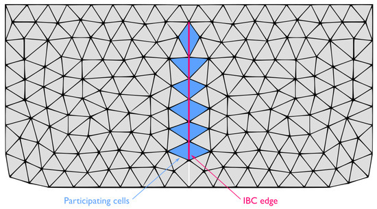
Figure 4.
Internal boundary cells.
Assuming the pipe roof collapse has not occurred and the flow direction from left to right, the upstream element is cell L and the downstream is cell R. Water surface elevation levels at the left side , provided by the numerical scheme (21), are used to evaluate the discharge by means of the external discharge expression. First, the change in the pipe bottom elevation and width due to erosion are computed using (9) and (10) as:
where accounts for the erosive shear stress at the breach evaluated at the time level . Then, the driving and the soil resistant forces, and , respectively, are computed using Equation (11), and the pipe roof collapse condition is checked. Therefore, two cases must be taken into consideration:
- (1)
- If the roof collapse does not occur, the pipe is considered filled with water and pressurized so that the enforced cell discharge in pipe during the next time level is computed using (7) as:where the integrated breach features A, f, L, R are evaluated at time ;
- (2)
- If the roof collapse condition is satisfied, the dambreach is assumed open and the enforced cell discharge in pipe during the next time level is computed using (8) as:
Note that once the roof collapse occurs, the pipe stability condition does not need to be checked any more, and the dam breach is assumed open. Regardless of whether the pipe is maintained or collapsed, the unit discharge at each cell pair composing the dambreach is assumed normal to the direction of the shared edge , and its module is updated as:
where is the total breach width and l is the length of the shared edge for each internal boundary cell pair.
3. Numerical Results and Discussion
3.1. Test Case 1: Synthetic Dambreach through Piping Process
The purpose of this first test case is to validate the performance of the model at the time of the collapse that leads to the transition from piping to dambreach. The case consists of a reservoir of 7 million cubic metres of water contained by a m high dam. At a given instant ( s), the dam will start to crack due to the piping mechanism. Figure 5 Left shows the topography of both the bottom of the reservoir and the domain through which the water will flow. Figure 5 Right shows the 4000 cells unstructured computational mesh used to discretize the domain. A more refined mesh has not been considered due to the purpose of the case does not require it.
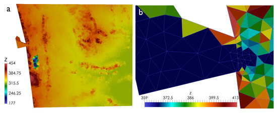
Figure 5.
Bed level (a) and detail of the dam geometry together with the triangular computational mesh (b).
Figure 6 shows the distributed numerical results for the water depth at the initial state, h, h, h, h and h, respectively. The results show a correct and stable temporal update of the water depth both inside and outside the reservoir through the flow through the breach estimated by means of the Equations (7) and (8).
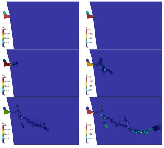
Figure 6.
Temporal evolution of the surface water depth h after the dam breach at the initial state, h, h, h, h and h, respectively.
On the other hand, Figure 7, Figure 8 and Figure 9 show the temporal evolution of the breach water discharge Q, top (B) and bottom (b) pipe/breach width and top () and bottom level (), respectively. In this particular case, the collapse occurs moments after the beginning of the piping process, at h approximately, due to the upper limit of the breach has reached the crest of the dam (Figure 9). Figure 7 (lower) shows a detail of the abrupt change in breach flow around the collapse time. At h approximately, the breach expansion stops due to the limits imposed by the case topography (Figure 8). After that, the breach discharge present minor fluctuations due to the 2D flow present within the reservoir, which causes variations in the upstream water level and, thence, in the breach discharge. As the level of the reservoir decreases, the water flow through the breach also does leading to an hydrograph consistent with those reported in the numerical tests and in the experiments of Chen et al. [16].
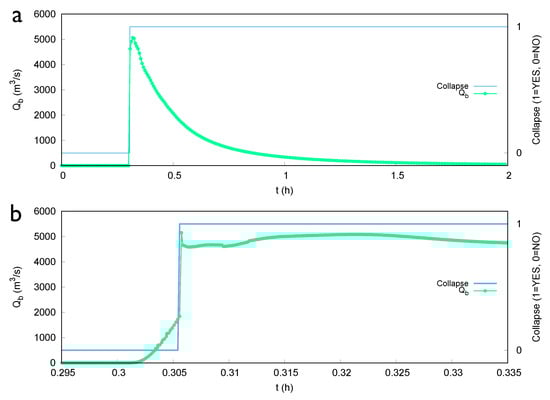
Figure 7.
Pipe/breach discharge (Q) temporal evolution for a piping starting time h. Full simulation time (a) and detail at the collapse time (b).
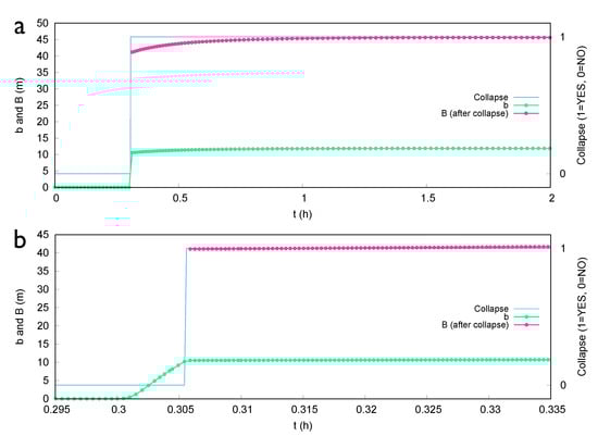
Figure 8.
Temporal evolution of the top (B) and bottom (b) width of the breach for a piping process starting at time h. Full simulation time (a) and detail at the collapse time (b).
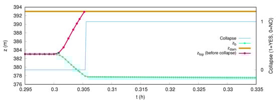
Figure 9.
Temporal evolution of the top () and bottom level () of the breach for a piping process starting at time time h.
3.2. Test Case 2: Synthetic Set of Dams
The following test case consists of a collection of synthetic dams with different characteristics and was originally presented in [23]. The main goal of this set of cases was to simulate a representative range of United States Department of Agriculture (USDA) small watershed structures by varying the dimensions (height and volume) of the reservoir and dam material composition. In [23], the simulations were performed using the software WinDAM C, developed by USDA Natural Resources Conservation Service (USDA-NRCS) in cooperation with USDA Agricultural Research Service (USDA-ARS) and Kansas State University [24].
The shape of the reservoirs can be described by a hypsometric function [23] as follows:
where h represents the reservoir depth, relative to the base of the dam, is the maximum depth, is the volume of water within the reservoir at depth h, and the maximum volume. This reservoir shape can be visualized as a cone with vertex at the bottom of the reservoir and the base defined by the water surface (see Figure 10).
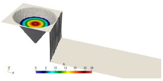
Figure 10.
Three-dimensional view of the Test Case 2 geometry.
Regarding the dam geometry, the set of cases includes six different heights and widths for the dam crest. The dimensions are included in Table 1 both using the unit system found in [23] and using the IS of units as used in our calculations. As stated in [23], a single length value of 274 m was set for all the cases as the average of the median lengths of the real world cases. Finally, a ratio of 3:1 was selected for upstream and downstream slopes, according to the US Bureau [25].

Table 1.
Set of dam heights and widths for Test Case 2.
Three different characterizations of the dam material have been considered (see Table 2), with the erodibility and the critical shear stress being the most notable parameters for WinDAM C software [23]. Equation (7) also requires the median particle size in mm for predicting the breach water discharge.
Table 2.
Set of dam material parameters for Test Case 2.
Regarding the initial conditions, the internal erosion was assumed to be initiated with a void square in cross section and having dimensions of 6.1 cm high and 6.1 cm wide, located at the centreline of the dam and at elevation coinciding with above of dam base.
Figure 11 shows the details of the computational mesh and dam breach line for this test case. The mesh consists of 23,355 triangular cells, which ensures a good representation of the geometry of the dam.
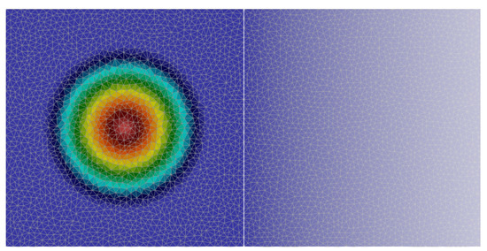
Figure 11.
Details of the computational mesh and dam breach line for Test Case 2.
Figure 12 shows the numerical results in logarithmic scale obtained for the breach peak discharge in the 18 simulated cases (six geometries × three dam materials). They are labelled as High, Medium and Low, corresponding to the previously defined material characteristics. The results provided by WinDAM C are also shown, extracted from [23]. In general, the same linear trends are observed for both models although the two-dimensional model predicts slightly higher values for the breach discharge than WinDAM C, especially for intermediate and high dam height values. The maximum discrepancy between both models appears in the 8 ft tall dam with the medium parameter set, with a relative difference of , and for the minimum, also in the 8 ft tall dam, but choosing the high parameter set with a relative difference of .
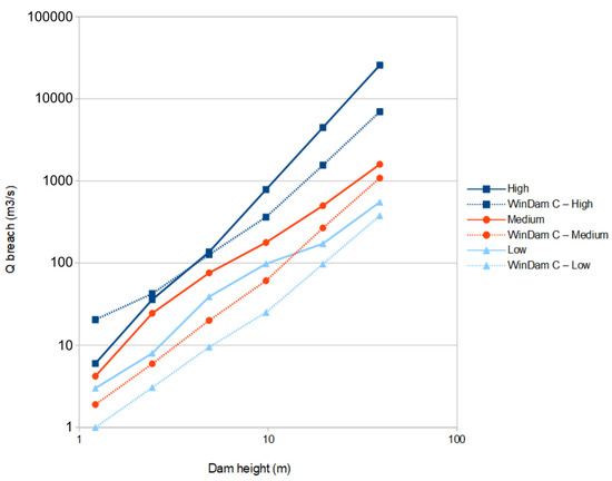
Figure 12.
Peak breach discharge as a function of dam height for synthetic sets (continuous line) and comparison with the results provided by WinDam C (dashed line).
Regarding the computational efficiency, the computational costs of the implementation of the model in GPU (two different GPU cards were tested) have been compared with the CPU model for this particular case, using the Low parameter set. The reason for choosing this set of parameters to perform this comparison is the slower evolution of the breach and, therefore, the longer simulation time required to reach the peak breach discharge. Table 3 shows the calculation times for both models, together with the speed-up factor, computed as the gain ratio with respect to the one-core CPU computational time.
Table 3.
Computational times for GPU and CPU models and the speed-up factor. GPU1 = NVIDIA GeForce GTX Titan Black (NVIDIA Corporation, Santa Clara, CA, USA), GPU2 = NVIDIA GeForce GTX 1080Ti (NVIDIA Corporation, Santa Clara, CA, USA), CPU = Intel Core i7-3770K (Intel Corporation, Santa Clara, CA, USA).
4. Conclusions
In this work, the improvement of RiverFlow2D-GPU, a surface flow model based on 2D Shallow Water equations with a dambreach piping utility, has been presented. The overflow dambreach situation is also considered in the model. The dam is defined as an internal boundary condition where the operation conditions take into account all the possible hydraulic scenarios. The model is able to develop a transient water flow all over the computational domain, including the reservoir and the downstream valley at the same time. Every time step, the discharge through the dam is updated according to the flow conditions in order to obtain a perfect tracking of the dambreach evolution. Two applications at different spatial scales have been shown for validation of the model and to test the efficiency of the GPU implementation. The first case was used to validate the performance of the model at the time of the collapse that leads to the transition from piping to dambreach. The results are consistent with those reported in the numerical tests and in the experiments. Additionally, both CPU and GPU models provide exactly the same numerical results. A very good agreement was shown as well as good GPU efficiency. The second case consists of a collection of synthetic dams with different characteristics. The main goal of this set of cases was to simulate a representative range of United States Department of Agriculture (USDA) small watershed structures by varying the dimensions (height and volume) of the reservoir and dam material composition. The results provided by WinDAM follow the same linear trends observed in our model in general. The main conclusion of the present work is the successful enhancement of the 2D shallow water flow model RiverFlow2D-GPU by means of dynamic internal boundary conditions that allow the simulation of the evolution of dam breach processes, as well as the propagation of the subsequent overland flow waves. Additionally, the results obtained in this work support the generalized paradigm shift that is taking place within the scope of hydraulic simulation. The use of GPUs against CPUs, especially in computational meshes with a large number of cells, provides significant gains in simulation efficiency. In particular, to the authors’ knowledge, no previous works consider either GPU computing for a 2D model including a dynamical internal boundary condition of the dam breach type.
Author Contributions
Conceptualization, S.M.-A. and P.G.-N.; methodology, S.M.-A.; software, S.M.-A. and J.F.-P.; validation, S.M.-A. and J.F.-P.; resources, P.G.-N.; data curation, J.F.-P.; writing—original draft preparation, S.M.-A.; writing—review and editing, J.F.-P. and P.G.-N.; supervision, P.G.-N.; funding acquisition, P.G.-N. All authors have read and agreed to the published version of the manuscript.
Funding
This work was partially funded by the University of Zaragoza under the research project JIUZ2022-IAR-03: High Performance Computing Tools for Smart Agriculture and Forestry.
Data Availability Statement
Not applicable.
Conflicts of Interest
The authors declare no conflict of interest.
Abbreviations
The following abbreviations are used in this manuscript:
| FV | Finite Volume |
References
- Wetmore, J.; Fread, D. The NWS Simplified Dam-Break Model; Technical Report; National Weather Service; NOAA: Washington, DC, USA, 1983. [Google Scholar]
- Fread, D. NWS FLDWAV Model: The replacement of DAMBRK for dam-break flood prediction. In Proceedings of the 10th Annual Conference of the ASDSO, Kansas, MO, USA, 26–29 September 1993; pp. 177–184. [Google Scholar]
- Albu, L.M.; Enea, A.; Iosub, M.; Breabăn, I.G. Dam Breach Size Comparison for Flood Simulations. A HEC-RAS Based, GIS Approach for Drăcșani Lake, Sitna River, Romania. Water 2020, 12, 1090. [Google Scholar] [CrossRef]
- Jiang, H.; Zhao, B.; Dapeng, Z.; Zhu, K. Numerical Simulation of Two-Dimensional Dam Failure and Free-Side Deformation Flow Studies. Water 2023, 15, 1515. [Google Scholar] [CrossRef]
- Mirauda, D.; Albano, R.; Sole, A.; Adamowski, J. Smoothed Particle Hydrodynamics Modeling with Advanced Boundary Conditions for Two-Dimensional Dam-Break Floods. Water 2020, 12, 1142. [Google Scholar] [CrossRef]
- Kocaman, S.; Güzel, H.; Evangelista, S.; Ozmen-Cagatay, H.; Viccione, G. Experimental and Numerical Analysis of a Dam-Break Flow through Different Contraction Geometries of the Channel. Water 2020, 12, 1124. [Google Scholar] [CrossRef]
- Dekay, M.; McClelland, G. Setting Decision Thresholds for Dam Failure Warnings: A Practical Theory-Based Approach; Technical Report No. 328; Center for Research on Judgment and Policy CRJP, University of Colorado: Boulder, CO, USA, 1991; 145p. [Google Scholar]
- Martínez-Aranda, S.; Fernández-Pato, J.; Echeverribar, I.; Navas-Montilla, A.; Morales-Hernández, M.; Brufau, P.; Murillo, J.; García-Navarro, P. Finite Volume models and Efficient Simulation Tools (EST) for Shallow Flows. In Advances in Fluid Mechanics: Modelling and Simulations; Springer Nature: Singapore, 2022; ISBN 978-9-81191-437-9. [Google Scholar]
- Lacasta, A.; Morales-Hernández, M.; Murillo, J.; García-Navarro, P. An optimized GPU implementation of a 2D free surface simulation model on unstructured meshes. Adv. Eng. Softw. 2014, 78, 1–15. [Google Scholar] [CrossRef]
- Echeverribar, I.; Martínez-Aranda, S.; Fernández-Pato, J.; García-Navarro, P. A GPU-based 2D viscous flow model with variable density and heat exchange. Adv. Eng. Softw. 2023, 175, 103340. [Google Scholar] [CrossRef]
- Martínez-Aranda, S.; Murillo, J.; García-Navarro, P. A GPU-accelerated Efficient Simulation Tool (EST) for 2D variable-density mud/debris flows over non-uniform erodible beds. Eng. Geol. 2022, 296, 106462. [Google Scholar] [CrossRef]
- Fernández-Pato, J.; García-Navarro, P. An efficient GPU implementation of a coupled overland-sewer hydraulic model with pollutant transport. Hydrology 2021, 8, 146. [Google Scholar] [CrossRef]
- Gordillo, G.; Morales-Hernández, M.; Echeverribar, I.; Fernández-Pato, J.; García-Navarro, P. A GPU-based 2D Shallow Water quality model. J. Hydroinformatics 2020, 22, 1182–1197. [Google Scholar] [CrossRef]
- Cunge, J.A.; Holly, F.M.; Verwey, A. Practical Aspects of Computational River Hydraulics; Pitman Pub. Inc.: Wetherby, UK, 1989. [Google Scholar]
- Arcement, G.; Schneider, V. Guide for Selecting Manning’s Roughness Coefficients for Natural Channels and Flood Plains; Number 2339 in U.S. Geological Survey; Water-Supply Paper, U.S.G.P.O (Government Publishing Office); For sale by the Books and Open-File Reports Section; U.S. Geological Survey: Reston, VA, USA, 1984. [Google Scholar]
- Chen, S.S.; Zhong, Q.M.; Shen, G.Z. Numerical modeling of earthen dam breach due to piping failure. Water Sci. Eng. 2019, 12, 169–178. [Google Scholar] [CrossRef]
- Wu, W. Simplified Physically Based Model of Earthen Embankment Breaching. J. Hydraul. Eng. 2013, 139, 837–851. [Google Scholar] [CrossRef]
- Fread, D. Dambreak: The NWS Dam Break Flood Forecasting Model; National Weather Services: Silver Spring, MD, USA, 1984. [Google Scholar]
- Singh, V. Dam Breach Modeling Technology; Kluwer Academic Publishes: Dordrecht, The Netherlands, 1996. [Google Scholar]
- Roe, P. Approximate Riemann solvers, parameter vectors, and difference schemes. J. Comput. Phys. 1981, 43, 357–372. [Google Scholar] [CrossRef]
- Morales-Hernández, M.; Murillo, J.; García-Navarro, P. The formulation of internal boundary conditions in unsteady 2-D shallow water flows: Application to flood regulation. Water Resour. Res. 2013, 49, 471–487. [Google Scholar] [CrossRef]
- Echeverribar, I.; Morales-Hernández, M.; Brufau, P.; García-Navarro, P. Use of internal boundary conditions for levees representation: Application to river flood management. Environ. Fluid Mech. 2019, 19, 1253–1271. [Google Scholar] [CrossRef]
- Tejral, R.; Hunt, S. Comparing process-based breach models for earthen embankments subjected to internal erosion. In Proceedings of the 5th Federal Interagency Hydrologic Modeling Conference and the 10th Federal Interagency Sedimentation, Reno, NV, USA, 19–23 April 2015. [Google Scholar]
- Hunt, S.; Temple, D.; Neilsen, M.; Ali, A.; Tejral, R. WinDAM C: Analysis Tool for Predicting Breach Erosion Processes of Embankment Dams Due to Overtopping or Internal Erosion. Appl. Eng. Agric. 2021, 37, 523–534. [Google Scholar] [CrossRef]
- Bureau of Reclamation U.B. Design of Small Dams; Technical Report; U.S. Governement Printing Office: Washington, DC, USA, 1987. [Google Scholar]
Disclaimer/Publisher’s Note: The statements, opinions and data contained in all publications are solely those of the individual author(s) and contributor(s) and not of MDPI and/or the editor(s). MDPI and/or the editor(s) disclaim responsibility for any injury to people or property resulting from any ideas, methods, instructions or products referred to in the content. |
© 2023 by the authors. Licensee MDPI, Basel, Switzerland. This article is an open access article distributed under the terms and conditions of the Creative Commons Attribution (CC BY) license (https://creativecommons.org/licenses/by/4.0/).