Article

Modelling Climate Change and Water Quality in the Canadian Prairies Using Loosely Coupled WASP and CE-QUAL-W2

by
Julie Terry
* and
Karl-Erich Lindenschmidt
Global Institute for Water Security, University of Saskatchewan, Saskatoon, SK S7N 3H5, Canada
*
Author to whom correspondence should be addressed.
Water 2023, 15(18), 3192; https://doi.org/10.3390/w15183192
Submission received: 5 August 2023 / Revised: 3 September 2023 / Accepted: 4 September 2023 / Published: 7 September 2023
(This article belongs to the Section Water Quality and Contamination)

Abstract

:
The prairie waterbodies face a future of warming temperatures and growing water demands. There are increasing concerns about how water quality will be affected. Water quality models are an effective tool for examining scenarios of future conditions that cannot be measured directly. This study combined WASP and CE-QUAL-W2 to investigate the potential impacts of changing flow management and climate change in the Canadian Prairies. The two models were loosely coupled to simulate a strategically managed river-reservoir network. Climate data from the Coupled Model Intercomparison Project Phase 6 (CMIP6) model ensemble were used to create future climate scenarios. Interbasin water transfers were then simulated through the coupled models to determine if any negative impacts from climate change on water quality could be offset through flow management. Climate change impacts in the river stretch were minimised due to the rapid flow travel time along the channel. The interbasin water transfers had a greater influence on water quality concentrations in the river. This result was limited by the uncertain hydro-climatic future of the contributing watershed. Climate change impacts in the downstream reservoir were far more apparent. Evaporative losses increased approximately 150% from the base model by the 2080–2100 period. Chlorophyll-a concentrations increased an average of 53% in this same period based on monthly mean percentage change. Reservoir water quality was improved after adding the interbasin water transfers. Results indicated that flow management would have a positive impact on water quality in the reservoir in the face of future climate change.

1. Introduction

Our freshwater resources are under stress. The unsustainable use of water has led to falling levels of groundwater, and loss of lakes, river flows, and wetlands [1,2]. Canada contains approximately nine percent of global available surface freshwater, and yet water resources are a concern [3]. Freshwater access is complicated by geographical variability and location of population centres [4]. In the South Saskatchewan River Basin (SSRB), a 336,000 km2 area that passes through the prairie regions of Alberta, Saskatchewan and Manitoba, agriculture is responsible for 82% of consumptive water use [5]. Water demands are expected to increase from irrigation expansion [6], and growth in the surrounding urban areas. This is a land subject to high economic losses from persistent floods and droughts [5,7]. Water security challenges in the SSRB basin include provision of sufficient water resources and drinking water quality concerns [8].
The prairie provinces are drylands laying in the rain shadow of the Rocky Mountains [4], yet flooding can occur during intense storm events or spring melt due to the flat landscape. Waterbodies can be frozen over half of the year influencing aquatic processes and restricting water transfer capacities in the highly managed waterways. Warmer temperatures are projected on the Prairies by the end of the 21st century [9], with air temperature being an important factor behind summer drought. Prairie waterbodies are often shallow, unshaded, and exposed to the wind—facilitating evapotranspiration and warming of the water column. Rising water temperatures can have negative impacts on reservoir water quality, such as faster algal growth, accelerated reaction rates, lower oxygen capacity of the water column, and stronger summer stratification layers. Urgent questions are being asked about how water quality in the region will respond to changing flow management and climate change.
Models are valuable tools to understand and predict future water quality under climate change. Models can examine scenarios and be used for assessment when conditions are not directly measurable. The inclusion of climate change impact assessments in water quality studies has developed worldwide, e.g., refs. [10,11,12,13]. General circulation model (GCM) output can be at a coarse temporal resolution for water quality models and can omit essential meteorological variables required for running simulations [14]. Regional climate models (RCM) can be used to downscale the large-scale output of GCMs to smaller, more catchment-sized grid cells [15]. Even at these smaller scales, care must be taken when incorporating the climate model data into the water quality model. Climate model output will show significant bias when comparing baseline values to known observations taken from a local weather station. Sources of bias include inherent uncertainty in GCM output representing large-scale processes in coarse grid cells, as well as systematic errors due to GCM and RCM model structures. This bias is usually determined by the modeller, and techniques range from simple scaling to complex statistical approaches. Comprehensive reviews of bias correction methods have been made by other authors, e.g., refs. [15,16,17].
This paper examines the potential impacts of climate change on water quality in the prairie provinces of Canada. Climate scenarios are developed for a prairie river-reservoir system simulated in the loosely coupled water quality models WASP and CE-QUAL-W2. A simple delta change approach is used for bias correcting the climate data. Delta change is a widely used scaling method, employed to evaluate a model’s response to climate change [16]. This paper also adds a water management perspective to the climate scenarios by evaluating the potential for interbasin water transfers to offset any negative impacts of climate change on downstream water quality.

2. Methods

2.1. Study Site

Located in the Upper Qu’Appelle River Basin, Buffalo Pound Lake (BPL) receives water from the South Saskatchewan River Basin through managed interbasin transfers from Lake Diefenbaker (Figure 1). An important drinking water resource, BPL provides water for approximately 25% of the provincial population of Saskatchewan. Water demands on this impounded natural lake include municipal, industrial, agricultural, and recreational use. In recent years, operating costs have increased for the on-site Buffalo Pound Water Treatment Plant (BPWTP) due to poor quality source water from overland runoff, and algal bloom development.
The Upper Qu’Appelle River connects Lake Diefenbaker to downstream BPL along a 97 km channel that is part improved channelised river (upper 35 kms) and meandering natural river channel (lower 62 km). Discharge in the channel can be rapid with a calculated travel time of under 2 days in high flows [18]. Water levels in the Upper Qu’Appelle River system are carefully managed to avoid flooding the flat landscape of the Qu’Appelle Valley. Water transfers between Lake Diefenbaker and BPL must be maximised while accounting for channel capacity and the amount of overland runoff already contributing to the system. In very wet years and during the spring freshet, transfers from Lake Diefenbaker may be reduced substantially. BPL residence time is highly variable at 6 to 36 months [19], in part due to the need to carefully control water levels. On rare occasions, flood waters of poorer water quality, from Moose Jaw Creek downstream, can backflow over the gates of the outflow dam and into the reservoir.
Daily average air temperatures in the area range from −17.7 °C to +26.2 °C, and approximately 30% of an annual mean precipitation of 365.3 mm falls as snowfall [20]. BPL is a cold polymictic lake under ice cover for around half of the year (range of 4.5 months to more than 6 months over a 39-year period, unpublished data), and that mixes frequently through the open water seasons.

2.2. Model Setup and Calibration

The climate change scenarios applied a loose coupling of WASP and CE-QUAL-W2 to model the changes in water quality in the Upper Qu’Appelle River and in BPL. Both models were originally developed as separate models for simulating water quality in the river (WASP) and reservoir (CE-QUAL-W2) (Figure 1). A later study loosely coupled the two models together to model the water quality impacts of increased water transfers from Lake Diefenbaker to BPL [21]. The coupling was to simulate nutrient transformations in the water transfers as they traversed the 97 km river stretch. Both models were calibrated and tested for the period from April 2013 to December 2019 for this prior study, making them ideal base models for assessing the potential impacts of climate change and flow management. The base model configurations were retained for this current study, with the focus being on the inclusion of climate change and flow management data for scenario analysis.
The setup described in the following sections refers to a two-step process where the climate change scenarios were first simulated in the Upper Qu’Appelle River in WASP, and then in BPL in CE-QUAL-W2. The WASP model output became the input boundary data for inflows and water quality for CE-QUAL-W2. The meteorological input files in both models were replaced with the climate scenario data. Once the climate scenarios were complete, one set of the climate change scenarios was run for a second time, but with added water transfers from Lake Diefenbaker. For this second part, the inflow data were replaced in the WASP model (as well as the climate data), and the new WASP outflows were then used as inflows for CE-QUAL-W2. The loose coupling setup meant nutrient transformations in the 97 km river stretch would again be simulated in the additional water transfers as per the base models.

2.2.1. WASP (River)

WASP (Water Quality Analysis Simulation Program) is a surface water quality model developed and maintained by the US Environmental Protection Agency and first released in 1981 [22]. The model is primarily a fate and transport model and has modelled contaminants in a range of different waterbodies over the decades in the USA and internationally [23]. The original Upper Qu’Appelle River model was built as a one-dimensional (1D) grid in WASP version 7 for a period ending in 2015 [24]. The time period was later extended until December 2019 when it was coupled to the BPL reservoir model [21]. Descriptions of the data, calibration procedure, and final model coefficients are provided in detail in these previous works. To summarise here, the WASP river section consisted of 165 longitudinal segments of approximately 600 to 800 m. The segmentation was originally determined from a HEC-RAS model provided by the Saskatchewan Water Security Agency (WSA). Inflow from nine tributaries join the main river flow network.
Data for calibration had been provided by the WSA for flow and water quality data, and Environment Canada and Climate Change (ECCC) and NOAA for meteorological data. Flow and meteorological data were both high-frequency datasets (hourly to daily), but water quality data ranged from daily to monthly in the open water season and infrequently in winter due to the challenges of sampling under ice cover.

2.2.2. CE-QUAL-W2 (Reservoir)

CE-QUAL-W2 is a two-dimensional (2D) complex hydrological and ecological model that has been applied to waterbodies worldwide since its release in 1986 by the US Army Corps of Engineers [25]. Since then, the model has been in continuous development by the Water Quality Research Group of Portland State University. CE-QUAL-W2 has successfully simulated the water quality in BPL for 2013–2019 in two earlier studies [18,21]. Full descriptions of model calibration, data sources, parameter values, and presentation of calibration results are provided in these previous works. Again, to summarise here, the 2D BPL model grid consisted of 100 longitudinal segments of approximately 300 m, and up to 28 vertical layers of 0.25 m in depth. The bathymetry was determined using a digital elevation model created in ArcGIS from sonar depth measurements.
Data for calibration were provided by the WSA and BPWTP for flows and water quality data, and ECCC for meteorological data. The most recent BPL modelling study was the coupling of WASP and CE-QUAL-W2. WASP output from the most downstream segment of the model was converted manually to input boundary data for the BPL model. This loosely coupled setup was continued in this current work. As per the WASP data, inflow and meteorological data were high-frequency measurements (hourly to daily). Observations for the reservoir dam outflows and water abstraction had frequencies of approximately 1 month. Weekly, quality controlled, in-reservoir water quality data were provided from the BPWTP for their intake location near the downstream end of the reservoir. The WSA also provided supplemental water quality profile data for various sampling locations around the reservoir.
Calibration coefficients and parameters relevant to the climate change scenarios for both base models are included in Table 1 for comparative interest.

2.3. Climate Change Scenarios

2.3.1. Climate Data

Climate data from the Coupled Model Intercomparison Project Phase 6 (CMIP6) were used in this study. CMIP6 is the latest multi-model ensemble of the World Climate Research Programme and provided the scenarios of the 2021 Intergovernmental Panel on Climate Change (IPCC) sixth assessment report (AR6). Emission scenarios in AR6 are known as Shared Socioeconomic Pathways (SSPs). These SSPs are updated versions of the previously known Representative Concentration Pathways (RCPs) of the 2013 IPCC fifth assessment report (AR5) and CMIP Phase 5 (CMIP5). The SSPs share a common historical reference period until 2014, with the scenarios commencing from 2015 to 2100. Two CMIP6 pathways, SSP2-4.5 and SSP3-7, were chosen to represent the future climate in this study. SSP2-4.5 is considered an intermediate greenhouse gas (GHG) emissions scenario with CO2 emissions remaining at current levels to 2050 and then steadily declining towards 2100 as mitigation measures take affect (IPCC, 2021). The SSP3-7 pathway chosen for this study is a new scenario introduced with CMIP6 to represent a middle ground in the medium-high end of the forcing pathways. The highest end pathway of the emissions scenario is SSP5-8.5 (RCP8.5 in CMIP5)—A worst case scenario where humanity continues its current emissions trajectory with no corrective action taking place, but is considered somewhat implausible [26] (Hausfather & Peters, 2020).
The climate data were downloaded via Copernicus (Copernicus Climate Change Service, 2021) in NetCDF4 format and extracted using MATLAB. All climate variables were taken from the CMIP6 ensemble model ACCESS-CM2 and are shown in Table 2. ACCESS-CM2 has a grid resolution of 1.25° latitude by 1.875° longitude [27]. Limits of latitude and longitude for the sub-region extraction bounds for the Copernicus download site were 50° North, 51° South, −106° West, and −105° East.
Dew point was not directly available from ACCESS-CM2 and was calculated from air temperature and relative humidity using the Magnus formula in Equation (1), as per Lawrence [28], where coefficients A1 = 17.625, and B1 = 243.04 °C.
t d e w = B 1 l n R H 100 + A 1 t B 1 + t A 1 l n R H 100 A 1 t B 1 + t
Solar radiation was assumed to be the net balance of downwelling minus upwelling shortwave radiation. The original setup and calibration of the two models had treated solar radiation and cloud cover differently. In the WASP setup, shortwave solar radiation was included as a timeseries variable, along with fraction of daily light, but the cloud cover option was not used. In the CE-QUAL-W2 setup, cloud cover was included as a timeseries variable, but shortwave radiation was calculated internally by CE-QUAL-W2. Longwave radiation was computed internally by both models.
Wind direction is required for running CE-QUAL-W2 but was not available as a climate model variable. Climate change runs used the observed wind direction data as per the calibrated CE-QUAL-W2 base model.

2.3.2. Bias Correction

A common bias correction method is the delta change method [17]. With this method, climate model output for both a baseline and future period is compared and the ‘delta change’ is the calculated change between the two time periods. This delta change is then applied to the observed meteorological data to ‘scale’ to future climate conditions [17]. The absolute delta change is a simple subtraction of the baseline from the future as per Equation (2), where Δ = delta change.
i = C M I P 6   f u t u r e i C M I P 6   r e f e r e n c e i
The new meteorological timeseries in the water quality model then becomes the observed data plus the difference in climate as per Equation (3), where met = meteorological input file.
m e t   s c e n a r i o i = m e t   o b s e r v e d i + i
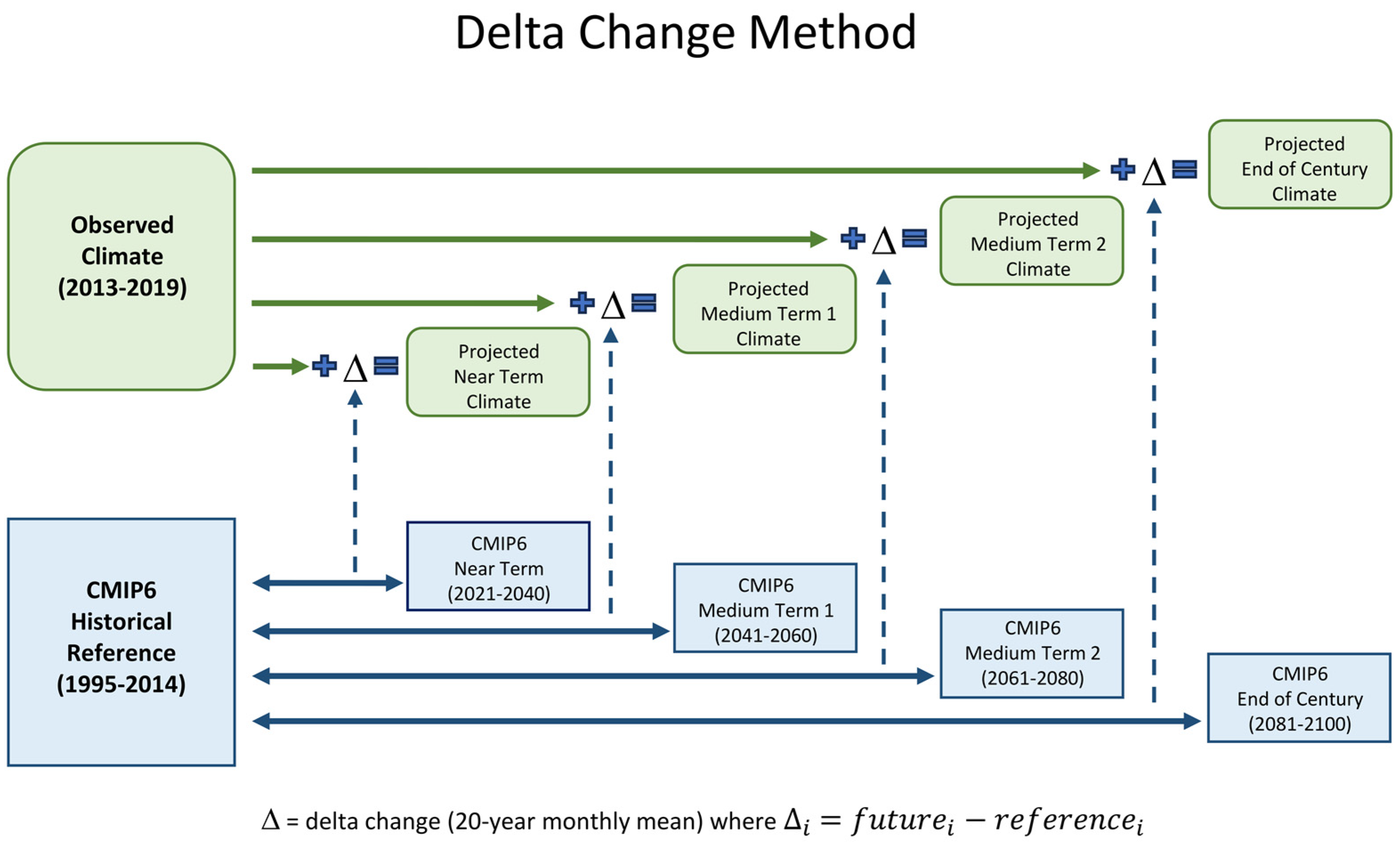
Four future time periods (near term (NT): 2021–2040, medium term: (MT1) 2041–2060 and (MT2) 2061–2080, end of century (EC): 2081–2100), and one historical reference period (1995–2014) were selected based on the CMIP6 Canadian Climate Data and Scenarios (CCDS) [29]. The ‘delta change’ for the purposes of this study was calculated as the difference between the 20-year monthly means to correspond with the monthly frequency of three of the climate variables (Table 2). Deltas were calculated for both the SSP2-4.5 and SSP3-7 pathways. Figure 2 depicts a schematic of the delta change bias correction that was performed.
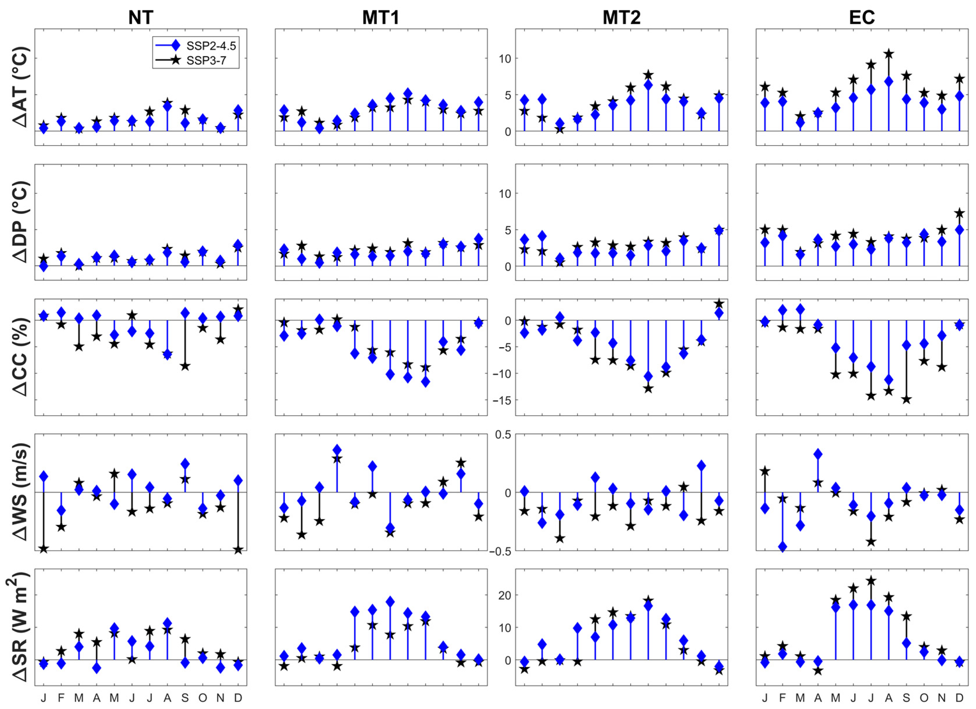
The ACCESS-CM2 climate model predicted that the climate would get hotter, with increased solar radiation and lower cloud cover. This trend intensified towards the end of the century and was the same for both pathways. SSP3-7 showed a greater display of change, as would be expected based on the criteria of the pathways. Wind speed was more variable but indicated a general decrease in the last two time periods. Figure 3 presents the calculated deltas.
The meteorological timeseries of the WASP and CE-QUAL-W2 base models, based on observed data from 2013 to 2019, were scaled to the four future periods by adding the appropriate delta change to the base model values (as depicted in Figure 2). The meteorological data were daily frequency in the base models; therefore, the delta change, which was calculated as a monthly mean difference, was assumed to be the same for each calendar day of the month. It was also assumed that the delta changes would stay constant each year of the simulation period (e.g., all Decembers were scaled with the same delta change factor). Note that the meteorological file in the calibrated CE-QUAL-W2 base model had contained hourly data, but this was averaged to daily for the climate change study due to the frequency of the CMIP6 data.

2.4. Interbasin Water Transfers

Water transfers from Lake Diefenbaker to BPL were augmented for two aspects of the modelling. For the setup of each climate change scenario, the inflows for the WASP model (i.e., the water transfers leaving Lake Diefenbaker) were increased marginally. This was necessary for increasing the subsequent inflows to the downstream BPL model to account for evaporation loss due to higher air temperatures. While WASP simply calculates the cumulative flow leaving the final segment of the model grid, the CE-QUAL-W2 structure requires the user to enter hydrological data and agree the water balance for the model to run. The evaporation option is turned on for the BPL simulations, due to the importance of evaporation in this prairie waterbody, and this factors into the agreed water balance. In the initial attempts to run the climate change scenarios in the CE-QUAL-W2 model, the additional losses to evaporation were causing the model to ‘run dry’ in the upstream grid cells and terminating the simulation with an error code. For simplicity with the climate scenarios, the inflows into WASP were augmented by a fixed amount for each pathway: SSP2-4.5 (1% increase), SSP3-7 (1.5% increase), and with a stepped (or rolling) increase over the four time periods (e.g., for SSP3-7, NT flow = base flow + 1.5%, MT1 flow = NT flow + 1.5%, MT2 flow = MT1 flow + 1.5%, and EC flow = MT2 flow + 1.5%).
Following the initial climate change runs, a water management aspect was then added to the SSP3-7 scenarios. Lake Diefenbaker is fed by waters from the Canadian Rockies and has better water quality than the downstream BPL, which receives high nutrient inputs as runoff from its agricultural watershed. Previous work with the base models of this study ascertained that additional water transfers could offset negative impacts of watershed runoff on water quality in BPL [21]. The water transfers were augmented for a second time in this current study to investigate if the additional transfers would still improve BPL’s water quality under the added pressure of climate change. The transfers were simulated for only the SSP3-7 pathway as this was found to have a greater influence on water quality than the SSP2-4.5 pathway.
The preferred water management strategy found in the previous study was used again here. Transfers were based on the maximum design capacity of the Upper Qu’Appelle channel of 14 m3/s in the open water season [30]. Open water was assumed as being May-October based on historical ice cover records. Transfers were calculated in only the open water conditions as augmenting flows to the suggested maximum capacity of 6 m3/s in ice-covered conditions [30] had relatively little influence on water quality [21], yet would increase the risk of ice damage to the channel. Available flow capacity was calculated by using the cumulative flow at WASP’s most downstream segment after the initial climate change runs (i.e., the scenarios already contained the small percentage increase in flows discussed above). Assumptions were that the end segment would be the point of greatest discharge and that channel capacity was the same throughout the river stretch. The cumulative daily flows between May and October were rounded up to the nearest integer and then deducted from the maximum capacity of 14 m3/s. If the days had spare capacity, then this difference was added to WASP’s inflow file for that day. For the rest of the days, and from November to April, WASP’s inflow file was left unchanged. To aid the water balance in CE-QUAL-W2, the water transfers were also added to the BPL dam outflow file for the purpose of this study. Table 3 summarises the climate change and interbasin water transfer scenarios.

3. Results and Discussion

3.1. Climate Change Scenarios in WASP

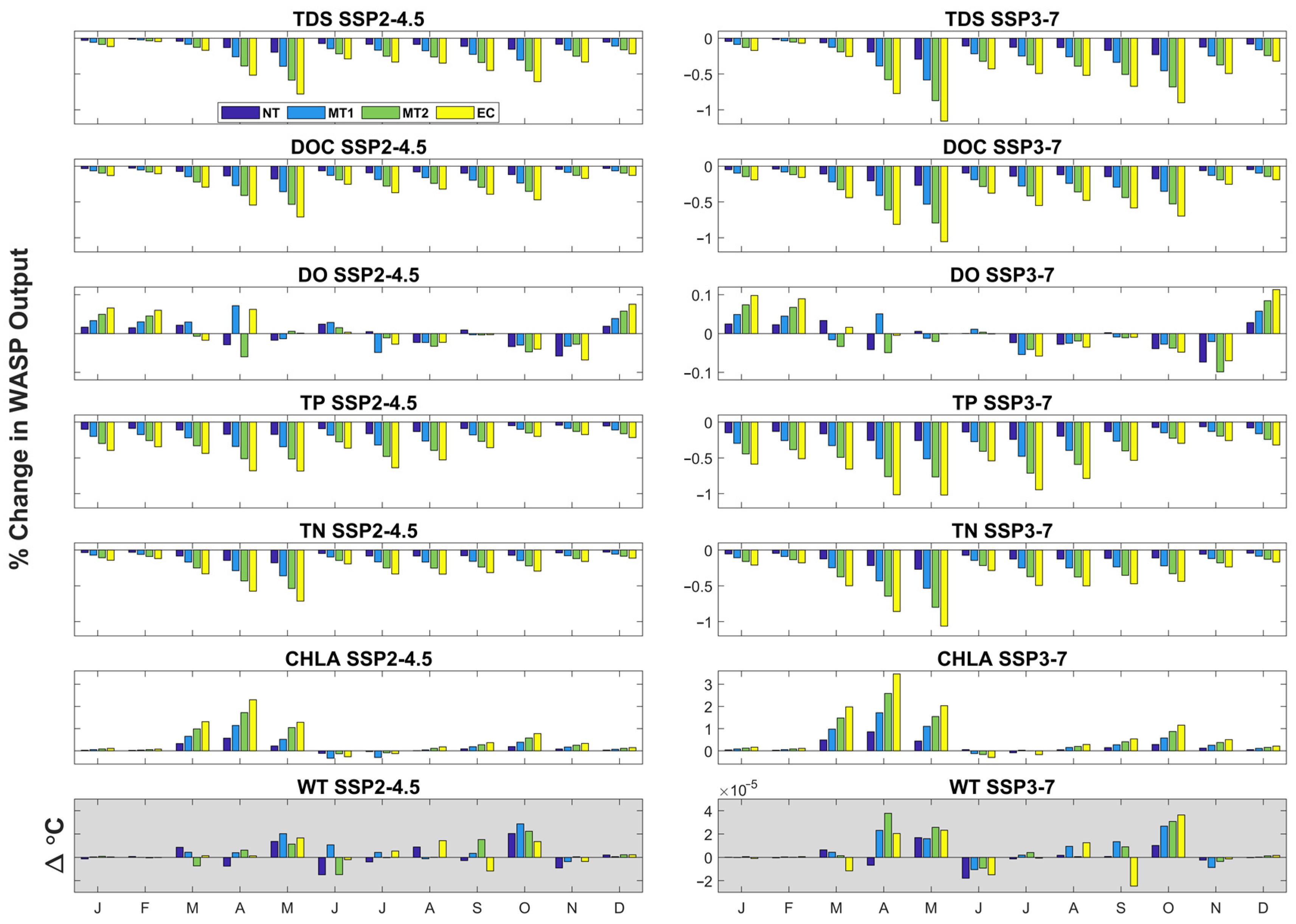
The impact of climate change was measured as being the percentage change between the base model and scenario model for six key water quality variables: total dissolved solids (TDS), dissolved organic carbon (DOC), dissolved oxygen (DO), total phosphorus (TP), total nitrogen (TN), and chlorophyll-a (CHLA). Results for the initial climate change scenarios are presented in Figure 4 for the most downstream segment in the WASP model. In this plot, daily percentage change over the 81 months of the simulation have been grouped using month of the year. The absolute change in simulated Water Temperature (WT) is also presented in Figure 4 for reference (grey plots). Monthly mean concentrations for the base model for the 81 months are given in Table 4. The results in Figure 4 show the total percent change in the water quality variables from the values of Table 4 with each climate change scenario.
Impacts in the Upper Qu’Appelle River model from climate change appeared to be minor—an assumption based on the minimal percentage change in water temperature. This was likely a result of the relatively rapid travel time through the river stretch. Changes were more noticeable from the additional water transfers added to aid the water balance in CE-QUAL-W2, as discussed in Section 2.4. CHLA showed the greatest percentage change out of all the variables and increased most during the months of spring bloom. This is when the water transfers coming from Lake Diefenbaker have the highest concentrations of algae. DO showed increased concentrations in winter when the river is under ice cover and inflows are the main source of oxygen renewal. The remaining variable concentrations all decreased in the scenarios over the year, with the percentage change consistently greater with each scenario. This again suggests that the water transfers were influencing water quality. The better-quality water of Lake Diefenbaker was diluting the concentrations in the main Upper Qu’Appelle channel, and the dilution effect was stronger as the transfers were stepped up over the decades.

3.2. Climate Change Scenarios in CE-QUAL-W2

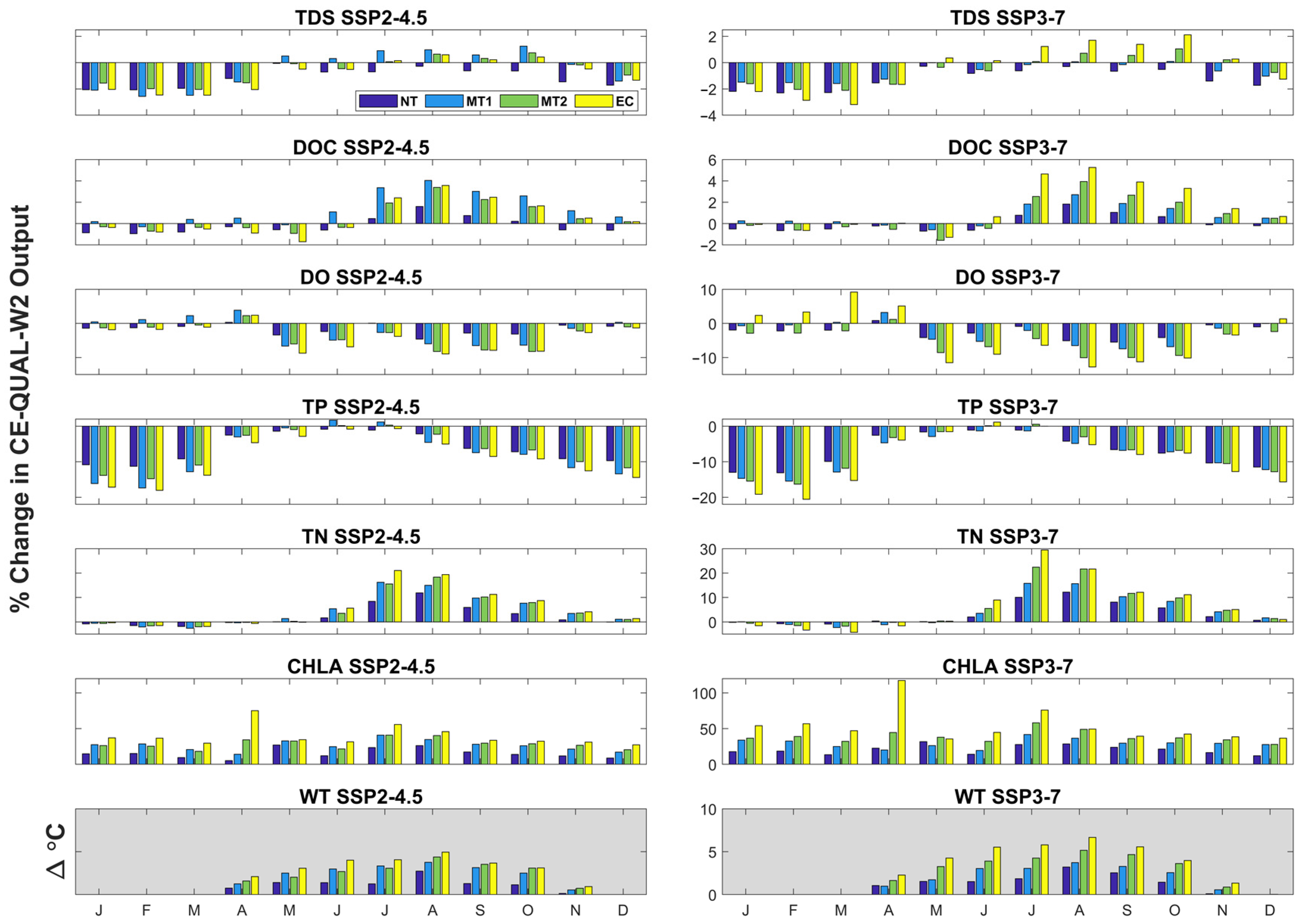
Results for the CE-QUAL-W2 BPL model are presented in Figure 5. To measure the climate change impact over the reservoir, model predictions were output for 20 longitudinal segments (segment 5, and then every fifth segment up to segment 100) at a daily frequency. The output file in CE-QUAL-W2 returned results for each layer of the requested segments, resulting in predictions for 215 grid cells over the model grid—the number of layers in a segment being dependent on the bathymetry depth at that location. Results for the variables were averaged over the 215 grid cells to one daily value that was used in the percentage change calculations presented here. Monthly mean concentrations for the base model for the 81 months are given in Table 5. The results in Figure 5 show the total percent change in the water quality variables from the values of Table 5 with each climate change scenario.
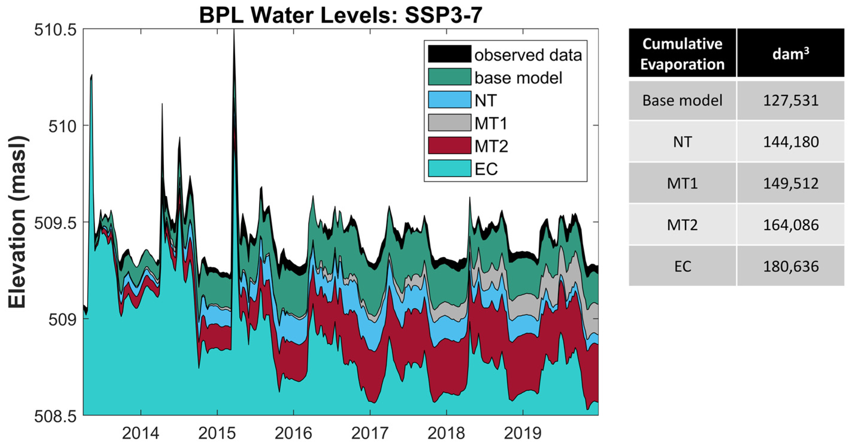
Impacts in the BPL model from climate change were much more pronounced. TDS can be considered a tracer constituent in CE-QUAL-W2 as the model has no internal sources or sinks for this variable [25]. The dilution of the water quality concentrations in the Upper Qu’Appelle River also occurred in BPL in winter when the model was simulating ice cover. During the open water period, the opposite occurred, and TDS concentrations increased from the base model. Figure 6 shows the simulated water levels close to the BPL dam, for the SSP3-7 scenarios. Also provided is total cumulative evaporation over the simulation period. These scenarios were after the stepped 1.5% increase in additional water transfers from Lake Diefenbaker (via WASP). Even with this additional inflow of water, increased evaporation due to rising temperatures indicated that the in-reservoir volume of water was reducing over each scenario. TDS appeared to be concentrating in the reservoir as a result.
DOC showed a similar pattern to TDS in the scenarios. With DOC, there would be additional contributions from organic materials such as dead algae, and allochthonous sources in the inflow constituent file. Water temperatures are directly influenced by air temperature [12], and rising air temperatures in the scenarios led to increased water temperatures as seen in Figure 6. This, in turn, would have led to faster rates of physio-chemical reactions such as mineralisation of organic matter and decay rates. Water temperatures also control the rate of algal growth leading to further organic materials in the water column. This explains why the percentage difference was even greater for DOC in summer than TDS and did not dilute as much in winter.
DO concentrations decreased in spring and summer with the higher water temperatures, as would be expected. Cold water can hold more oxygen and the DO saturation point decreases as temperatures rise. By the end of the century in SSP3-7, there was a jump in DO concentrations in March that would indicate an earlier onset of spring freshet flows, or an earlier ice-off date, and the subsequent oxygen replenishment. Total days of ice cover for the EC SSP3-7 scenario were 856, compared to 985 for the base model (NT = 941, MT1 = 919, and MT2 = 911). A corresponding spike in CHLA suggests that algal respiration may have also contributed to the higher DO.
TP decreases all year with the scenarios. TP was found to dilute with Lake Diefenbaker water transfers in the previous study [21]. In addition, the increase in algal blooms all year around, shown by CHLA, leads to greater uptakes of nutrients such as orthophosphate. In the warmer summer months, this reduction in TP from dilution and uptake is offset by the increased decay of organic materials in the model to the three constituent pools (nitrogen, phosphorus, and carbon).
This trend can also be seen in TN, which follows a similar temporal pattern to DOC with increased nitrogen from organic matter due to the warmer temperatures. Additional nitrogen concentrations also result from modelling nitrogen fixing species of cyanobacteria, which are present in BPL in mid-summer [31]. The CE-QUAL-W2 model was calibrated with three algal groups (representing diatoms, greens, and cyanobacteria). Algae are essentially limited by nitrogen and temperature in BPL as phosphorus is abundant. As water temperatures rise towards summer, the competitive advantage, based on temperature, switches to the cyanobacterial algal group in the model and the model simulates nitrogen fixation.

3.3. Climate Change Scenarios with Interbasin Water Transfers

Results for the CE-QUAL-W2 BPL model with the interbasin water transfers are presented in Figure 7. These are the same climate change scenarios as the previous section, but with maximised water transfers from Lake Diefenbaker in the open water season. The black lines within the coloured bars indicate the scenarios without the transfers (as per Figure 5) for comparison. The coloured bars in Figure 7 show the total percent change in the water quality variables from the values of Table 5 with each (SSP3-7) climate change and water management scenario.
In Figure 7, the results are presented for the grid cells representing the whole reservoir (20 longitudinal segments), and for the downstream quarter of the reservoir near the outflow dam (five longitudinal segments). The drinking water withdrawal pipes of the BPWTP are in this downstream section; therefore, water quality is of particular importance in this portion of BPL.
Based on the results for the overall reservoir, the water management transfers could mitigate the negative impact of climate change for almost all variables through dilution. The water temperatures are only slightly lowered with the additional inflows (the meteorological file has a greater influence on water temperature) and any reduction in physio-chemical reactions will be negligible in comparison. There is little change in the DO concentrations for this same reason. The spring bloom of CHLA is still strong in May with the additional inflows, although they are reduced for the remainder of the year.
The remaining variables are all shown to be significantly lowered by the augmenting of water transfers from Lake Diefenbaker. This agrees with the findings of the earlier research using the base models [21].
The modelling suggests that the benefits of the additional inflows would be lower over summer at the downstream end of the reservoir. Water age can be up to 3 years old by the time it reaches the BPL dam in normal operating conditions [19]. The meteorological conditions have had more time to influence water quality by this stage. Interestingly, TP increases greatly in May and June with the additional inflows. This may be due to increased sediment mobilisation and transport within the models from the higher discharge. Soluble P is strongly sorbed to bed sediments and suspended solids [32,33]. The ground and ephemeral streams of the Upper Qu’Appelle watershed are frozen until around April–May and newly mobilised sediments are transported through the Upper Qu’Appelle channel around this time. A more detailed spatial and temporal breakdown of the results would be a good way to determine the greatest contributing factors to nutrient loading and aid in management planning.

3.4. Limitations

A major limiting factor in a water quality climate change study is how to factor for hydrological unknowns. The water quality in BPL can be severely degraded by watershed runoff. This has been noted both in modelling studies and in empirical observations over the years. The hydrology of the watershed has also been described as incredibly complex, with a contributing area that varies depending on the amount of precipitation, and that functions on the percentage change between wet years and dry years (pers. comm. Chris Spence, Environment and Climate Change Canada). Additionally, there is a lack of hydrological observations for many of the intermittent and ephemeral streams contributing flow to the Upper Qu’Appelle River.
Climate change data are also highly uncertain by their very nature. Precipitation, in particular, has been difficult for climate models to agree on where locations will be wetter or drier, and when [34]. In the SSRB, the annual average precipitation is exceeded by the annual average evapotranspiration, and warming temperatures will likely lead to further evaporative losses and drier conditions [4]. Large declines in summer precipitation and streamflow may occur. In winter, warmer air temperatures will influence the transition from snowfall to rainfall [35] and shift the timing and quantity of spring melt from the watershed. Even increased precipitation could be offset by warmer temperatures intensifying evapotranspiration and reducing soil moisture and runoff [36]. Previous studies have found the Canadian Prairies to have an uncertain hydro-climatic future [7,37].
This study was limited to considering climate change variables that affect the heat balance equations. Precipitation was not considered in this study due to the high degree of uncertainty in climate model output for precipitation, and in how the Upper Qu’Appelle watershed runoff will change in the future. Similarly, this study assumes that the current volume of rainfall runoff in the watershed will be the same in future decades. If rainfall runoff does increase in the future, then greater amounts of nutrients will enter the reservoir than what has been modelled here. In addition, with greater amounts of runoff occurring, capacity in the Upper Qu’Appelle River channel will be reduced and there will be less opportunity to mitigate with better quality water from Lake Diefenbaker. Note, however, that the base models were calibrated to a recent period with a large degree of natural variability in precipitation.
Similarly, the delta change method assumes that trends in the baseline observed data for the included meteorological variables are likely to be maintained towards the future.
General limitations in the application of a water quality model (e.g., model structure, fixed or variable coefficients, mathematical equations), and specific uncertainties relating to the data for the Upper Qu’Appelle River and BPL research sites (e.g., boundary conditions, flows, spatial and temporal profiling) have been discussed in detail during the calibration stages of the base models, e.g., refs. [18,21,24,38].

4. Conclusions

WASP results suggested that climate change impacts on water quality in the Upper Qu’Appelle River will be mitigated through managed flows. The model had very little response to the changes in climate data. Travel time can be rapid in the Upper Qu’Appelle watershed and incoming discharge and constituents have far greater influence on water quality than the surrounding meteorological conditions. The results for the Upper Qu’Appelle model were not unexpected as an outcome. The main purpose of running the WASP model was for estimating nutrient transformations in the interbasin water transfers—with the climate change data added to the simulations for a complete analysis. Results from the WASP model were limited by the unknown hydro-climatic future of the Upper Qu’Appelle watershed. The potential for drastic changes in rainfall runoff in future decades should not be overlooked when interpreting the results.
Climate change impacts were far more apparent in the CE-QUAL-W2 reservoir model of Buffalo Pound Lake. Results of the climate change simulations highlight that a critical future concern may be the loss of reservoir volume to evapotranspiration. Water quality constituents were more concentrated in the remaining reservoir water in summer as a result. At the location of the drinking water intake pipe, this was true even with the addition of extra water transfers from Lake Diefenbaker in some cases, although sediment mobilisation due to the increased discharge may have contributed to the concentrations. Overall, model results indicated that augmented water transfers would have positive impacts on water quality in the reservoir even in the face of future climate change.
Water demands are anticipated to increase in the future in the Upper Qu’Appelle watershed. Greater transfers of water from the upstream South Saskatchewan River Basin will be required to keep Buffalo Pound Lake at operating supply level and maintain water quality. A prudent next step for water management would be to extend the modelling area to include Lake Diefenbaker and upstream to evaluate the future availability of water for these essential transfers.

Author Contributions

Conceptualisation, J.T. and K.-E.L.; funding acquisition, K.-E.L.; investigation, methodology, and analyses, J.T.; supervision, K.-E.L.; visualisation, J.T.; writing—original draft, J.T.; writing—review and editing, K.-E.L. All authors have read and agreed to the published version of the manuscript.

Funding

Funding for this project was provided by the University of Saskatchewan’s Global Water Futures Program.

Data Availability Statement

The authors do not have permission to share the third-party data used in this study.

Acknowledgments

The authors thank the Buffalo Pound Water Treatment Plant and the Saskatchewan Water Security Agency for providing the water quality data used to build and verify the model. The authors also thank Mohammed Ghoreishi at the Global Institute for Water Security for providing certain climate data. The University of Saskatchewan’s School of Environment and Sustainability and Global Institute for Water Security also provided data and technical support.

Conflicts of Interest

The authors declare no conflict of interest.

References

  1. Rodell, M.; Famiglietti, J.S.; Wiese, D.N.; Reager, J.T.; Beaudoing, H.K.; Landerer, F.W.; Lo, M.-H. Emerging trends in global freshwater availability. Nature 2018, 557, 651–659. [Google Scholar] [CrossRef]
  2. Wheater, H.S.; Gober, P. Water security and the science agenda. Water Resour. Res. 2015, 51, 5406–5424. [Google Scholar] [CrossRef]
  3. Watson, S.; Lawrence, J. Introductory remarks—Drinking water quality and sustainability. Water Qual. Res. J. Can. 2003, 38, 3–13. [Google Scholar] [CrossRef]
  4. Schindler, D.W.; Donahue, W.F. An Impending Water Crisis in Canada’s Western Prairie Provinces. Proc. Natl. Acad. Sci. USA 2006, 103, 7210–7216. [Google Scholar] [CrossRef] [PubMed]
  5. Wheater, H.; Gober, P. Water security in the Canadian Prairies: Science and management challenges. Philos. Trans. R. Soc. A Math. Phys. Eng. Sci. 2013, 371, 20120409. [Google Scholar] [CrossRef] [PubMed]
  6. Western Economic Diversification Canada. Prairie Prosperity: A Vision for the Management of Water Resources Across Saskatchewan and the Prairies; Western Economic Diversification Canada: Edmonton, AB, Canada, 2020; p. 27. [Google Scholar]
  7. Bonsal, B.R.; Cuell, C.; Wheaton, E.; Sauchyn, D.J.; Barrow, E. An assessment of historical and projected future hydro-climatic variability and extremes over southern watersheds in the Canadian Prairies. Int. J. Clim. 2017, 37, 3934–3948. [Google Scholar] [CrossRef]
  8. Masud, M.; Khaliq, M.; Wheater, H. Analysis of meteorological droughts for the Saskatchewan River Basin using univariate and bivariate approaches. J. Hydrol. 2015, 522, 452–466. [Google Scholar] [CrossRef]
  9. Bonsal, B.R.; Aider, R.; Gachon, P.; Lapp, S. An assessment of Canadian prairie drought: Past, present, and future. Clim. Dyn. 2013, 41, 501–516. [Google Scholar] [CrossRef]
  10. Fabian, P.S.; Kwon, H.-H.; Vithanage, M.; Lee, J.-H. Modeling, challenges, and strategies for understanding impacts of climate extremes (droughts and floods) on water quality in Asia: A review. Environ. Res. 2023, 225, 115617. [Google Scholar] [CrossRef] [PubMed]
  11. Elliott, J.A. Is the future blue-green? A review of the current model predictions of how climate change could affect pelagic freshwater cyanobacteria. Water Res. 2012, 46, 1364–1371. [Google Scholar] [CrossRef] [PubMed]
  12. Whitehead, P.G.; Wilby, R.L.; Battarbee, R.W.; Kernan, M.; Wade, A.J. A review of the potential impacts of climate change on surface water quality. Hydrol. Sci. J. 2009, 54, 101–123. [Google Scholar] [CrossRef]
  13. Quevedo-Castro, A.; Bustos-Terrones, Y.A.; Bandala, E.R.; Loaiza, J.G.; Rangel-Peraza, J.G. Modeling the effect of climate change scenarios on water quality for tropical reservoirs. J. Environ. Manag. 2022, 322, 116137. [Google Scholar] [CrossRef] [PubMed]
  14. Gelda, R.K.; Mukundan, R.; Owens, E.M.; Abatzoglou, J.T. A Practical Approach to Developing Climate Change Scenarios for Water Quality Models. J. Hydrometeorol. 2019, 20, 1197–1211. [Google Scholar] [CrossRef]
  15. Teutschbein, C.; Seibert, J. Bias correction of regional climate model simulations for hydrological climate-change impact studies: Review and evaluation of different methods. J. Hydrol. 2012, 456–457, 12–29. [Google Scholar] [CrossRef]
  16. Maraun, D. Bias Correcting Climate Change Simulations–A Critical Review. Curr. Clim. Chang. Rep. 2016, 2, 211–220. [Google Scholar] [CrossRef]
  17. Räty, O.; Räisänen, J.; Ylhäisi, J.S. Evaluation of delta change and bias correction methods for future daily precipitation: Intermodel cross-validation using ENSEMBLES simulations. Clim. Dyn. 2014, 42, 2287–2303. [Google Scholar] [CrossRef]
  18. Terry, J.; Davies, J.-M.; Lindenschmidt, K.-E. Buffalo Pound Lake—Modelling Water Resource Management Scenarios of a Large Multi-Purpose Prairie Reservoir. Water 2022, 14, 584. [Google Scholar] [CrossRef]
  19. Buffalo Pound Water Administration Board. Annual Report. 2015. Available online: https://www.buffalopoundwtp.ca/images/docs/2015_buffalo_pound_annual_report.pdf (accessed on 19 July 2017).
  20. Environment and Climate Change Canada. Climate Normals 1981–2010 Station Data for Moose Jaw A Station. Available online: http://climate.weather.gc.ca (accessed on 18 July 2023).
  21. Terry, J.; Lindenschmidt, K.-E. Water Quality and Flow Management Scenarios in the Qu’Appelle River–Reservoir System Using Loosely Coupled WASP and CE-QUAL-W2 Models. Water 2023, 15, 2005. [Google Scholar] [CrossRef]
  22. Wool, T.; Ambrose, R.B., Jr.; Martin, J.L.; Comer, A. WASP 8: The Next Generation in the 50-Year Evolution of USEPA’s Water Quality Model. Water 2020, 12, 1398. [Google Scholar] [CrossRef]
  23. Knightes, C.D.; Ambrose, R.B.; Avant, B.; Han, Y.; Acrey, B.; Bouchard, D.C.; Zepp, R.; Wool, T. Modeling framework for simulating concentrations of solute chemicals, nanoparticles, and solids in surface waters and sediments: WASP8 Advanced Toxicant Module. Environ. Model. Softw. 2019, 111, 444–458. [Google Scholar] [CrossRef] [PubMed]
  24. Hosseini, N.; Akomeah, E.; Davis, J.M.; Baulch, H.; Lindenschmidt, K.E. Water quality modeling of a prairie river-lake system. Environ. Sci. Pollut. Res. Int. 2018, 25, 31190–31204. [Google Scholar] [CrossRef]
  25. Wells, S.A. (Ed.) CE-QUAL-W2: A Two-Dimensional, Laterally Averaged, Hydrodynamic and Water Quality Model; Version 4.2, User Manual Parts 1–5; Department of Civil and Environmental Engineering, Portland State University: Portland, OR, USA, 2020. [Google Scholar]
  26. Hausfather, Z.; Peters, G.P. Emissions—The ’business as usual’ story is misleading. Nature 2020, 577, 618–620. [Google Scholar] [CrossRef] [PubMed]
  27. Bi, D.; Dix, M.; Marsland, S.; O’farrell, S.; Sullivan, A.; Bodman, R.; Law, R.; Harman, I.; Srbinovsky, J.; Rashid, H.A.; et al. Configuration and spin-up of ACCESS-CM2, the new generation Australian Community Climate and Earth System Simulator Coupled Model. J. South. Hemisphere Earth Syst. Sci. 2020, 70, 225–251. [Google Scholar] [CrossRef]
  28. Lawrence, M.G. The Relationship between Relative Humidity and the Dewpoint Temperature in Moist Air: A Simple Conversion and Applications. Bull. Am. Meteorol. Soc. 2005, 86, 225–234. [Google Scholar] [CrossRef]
  29. Government of Canada. The CMIP6 Multi-Model Ensembles Technical Documentation (Canada.Ca). 2023. Available online: https://climate-scenarios.canada.ca/?page=cmip6-technical-notes (accessed on 20 June 2023).
  30. Lindenschmidt, K.-E.; Sereda, J. The impact of macrophytes on winter flows along the Upper Qu’Appelle River. Can. Water Resour. J. 2014, 39, 342–355. [Google Scholar] [CrossRef]
  31. Painter, K.J.; Venkiteswaran, J.J.; Simon, D.F.; Duy, S.V.; Sauvé, S.; Baulch, H.M. Early and late cyanobacterial bloomers in a shallow, eutrophic lake. Environ. Sci. Process. Impacts 2022, 24, 1212–1227. [Google Scholar] [CrossRef] [PubMed]
  32. House, W.A. Geochemical cycling of phosphorus in rivers. Appl. Geochem. 2003, 18, 739–748. [Google Scholar] [CrossRef]
  33. Jarvie, H.P.; Jürgens, M.D.; Williams, R.J.; Neal, C.; Davies, J.J.; Barrett, C.; White, J. Role of river bed sediments as sources and sinks of phosphorus across two major eutrophic UK river basins: The Hampshire Avon and Herefordshire Wye. J. Hydrol. 2005, 304, 51–74. [Google Scholar] [CrossRef]
  34. Tapiador, F.J.; Roca, R.; Del Genio, A.; Dewitte, B.; Petersen, W.; Zhang, F. Is Precipitation A Good Metric for Model Performance? Bull. Am. Meteorol. Soc. 2019, 100, 223–234. [Google Scholar] [CrossRef] [PubMed]
  35. DeBeer, C.M.; Wheater, H.S.; Carey, S.K.; Chun, K.P. Recent climatic, cryospheric, and hydrological changes over the interior of western Canada: A review and synthesis. Hydrol. Earth Syst. Sci. 2016, 20, 1573–1598. [Google Scholar] [CrossRef]
  36. Martz, L.; Bruneau, J.; Rolfe, J. Climate Change and Water: SSRB (South. Saskatchewan River Basin). Final Technical Report; University of Saskatchewan: Saskatoon, SK, Canada, 2007. [Google Scholar] [CrossRef]
  37. Barrow, E.M.; Sauchyn, D.J. Uncertainty in climate projections and time of emergence of climate signals in the western Canadian Prairies. Int. J. Clim. 2019, 39, 4358–4371. [Google Scholar] [CrossRef]
  38. Terry, J.A.; Sadeghian, A.; Baulch, H.M.; Chapra, S.C.; Lindenschmidt, K.-E. Challenges of modelling water quality in a shallow prairie lake with seasonal ice cover. Ecol. Model. 2018, 384, 43–52. [Google Scholar] [CrossRef]
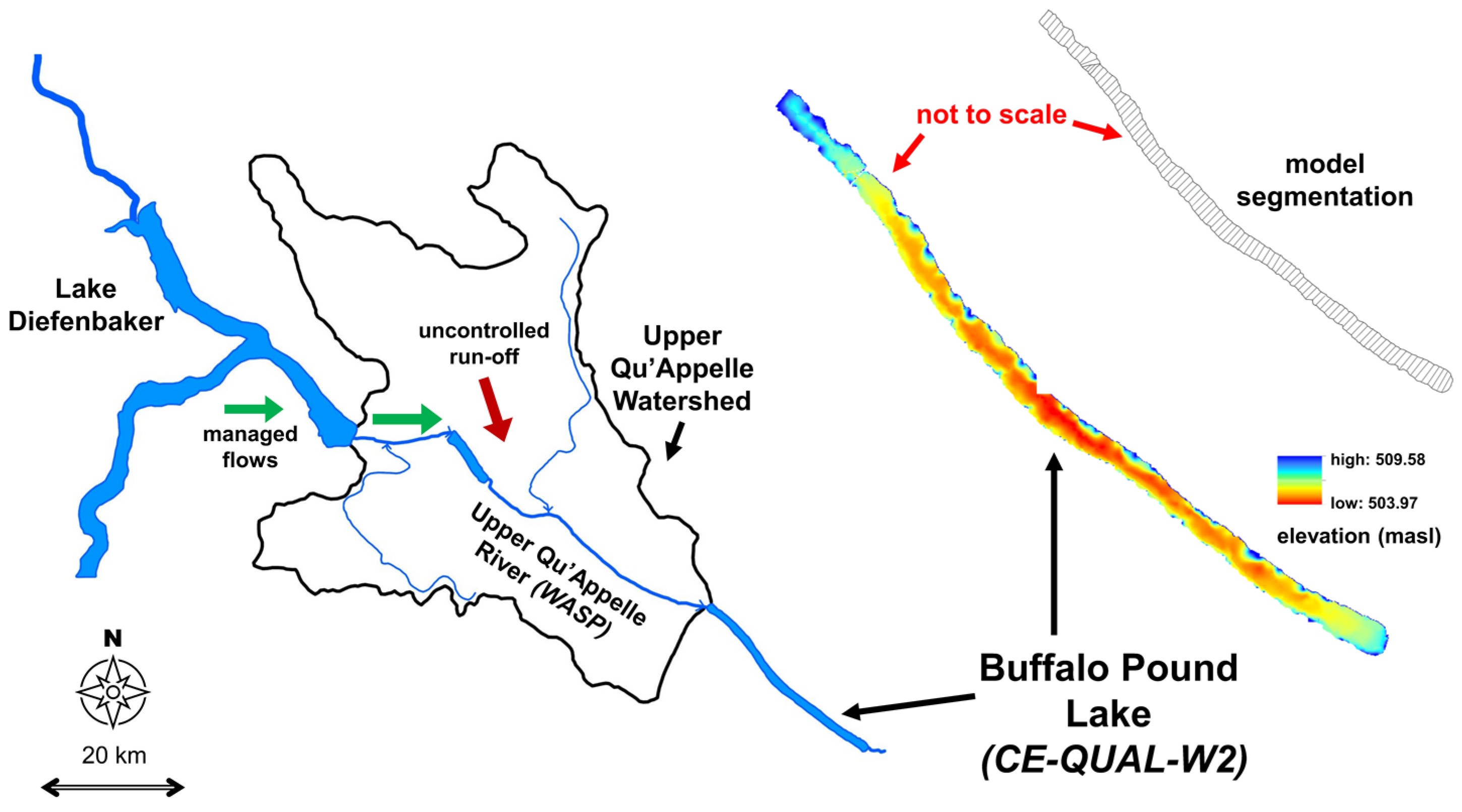
Figure 1. (Left) Map of the Upper Qu’Appelle watershed and river. Watershed outline taken from Terry et. al. [18]. (Right) Buffalo Pound Lake bathymetry and model grid in CE-QUAL-W2. The lake has a mean depth of 3.8 m, an average width of 890 m, and a total length of 30 kms.
Water 15 03192 g001
Figure 2. Conceptual diagram of the delta change method applied in this study. The blue boxes represent the calculation of the delta changes for each of the four future time periods. The resulting delta changes are then added to the observed climate data of the calibrated base model (large green box) to create new meteorological input files (i.e., the climate change scenarios). The dotted lines depict how the delta changes were added to the observed data for each time period.
Water 15 03192 g002
Figure 3. Calculated delta change values for CMIP6 pathways SSP2-4.5 and SSP3-7. The x-axis shows the months from January to December. The y-axis shows the 20-year, monthly mean delta changes for air temperature (AT), dewpoint temperature (DP), cloud cover (CC), wind speed (WS), and solar radiation (SR), where NT = 2021–2040, MT1 = 2041–2060, MT2 = 2061–2080, and EC = 2081–2100.
Water 15 03192 g003
Figure 4. WASP results for total dissolved solids (TDS), dissolved organic carbon (DOC), dissolved oxygen (DO), total phosphorus (TP), total nitrogen (TN), and chlorophyll-a (CHLA). The grey plots show the absolute difference for simulated water temperature (WT). The left-hand plots are for pathway SSP2-4.5, and the right-hand plots for pathway SSP3-7. Legend entries refer to the scenario time periods: near term (NT) 2021–2040, medium term (MT1) 2041–2060 and (MT2) 2061–2080, and end of century (EC) 2081–2100.
Water 15 03192 g004
Figure 5. CE-QUAL-W2 results showing the averaged percentage change over 215 grid cells of the reservoir model. Descriptions as per Figure 4.
Water 15 03192 g005
Figure 6. (Left): water levels in Buffalo Pound Lake (BPL) for each of the SSP3-7 pathway scenarios. The base model calibration years (x-axis) covered a natural wet period followed by relatively dry years. (Right): total cumulative evaporation over the model simulation period for each scenario.
Water 15 03192 g006
Figure 7. (Left): CE-QUAL-W2 results showing the averaged percentage change over 20 longitudinal segments after the addition of the maximised water transfers from Lake Diefenbaker (coloured lines). The climate change results prior to adding the maximised water transfers are shown for reference (black lines). (Right): the same results but shown for only five longitudinal segments representing only the most downstream section of the lake. Descriptions as per Figure 4.
Water 15 03192 g007
Table 1. A summary of parameters and coefficients in the calibrated WASP river and CE-QUAL-W2 reservoir base models.
DescriptionWASP (River)W2 (Reservoir)
Ice cover (default coefficients)ModelledModelled
Evaporation (default coefficients)Not modelledModelled
PrecipitationNot modelledModelled
Cloud CoverNot modelledObservations
Shortwave solar radiationObservationsInternally calculated
Longwave radiationInternally calculatedInternally calculated
Wind height measurement10 m above ground surface10 m above ground surface
Wind speed shelter coefficient10.9
Canopy shading coefficientNot modelled1
Algal groups13
Maximum growth rates (at 20 °C)3 (1/day)1.5\2\0.5
Minimum temperature for algal growth (°C)Internally calculated2\5\10
Optimum temperature range for algal growth (°C) Internally calculated8–15\20–35\35–40
Maximum temperature for algal growth (°C)Internally calculated24\40\50
Sediment oxygen demand (SOD)0.41 (g O2 m2/day)0.1–1.2 (g O2 m2/day)
Sediment release rate of phosphorus0 (mg/m2/day)0.015 (fraction of SOD)
Sediment release rate of ammonium0 (mg/m2/day)0.2 (fraction of SOD)
Nitrification rate (at 20 °C)0.01 (1/day)0.12 (1/day)
Denitrification rate (at 20 °C)0.09 (1/day)0.1 (1/day)
Table 2. CMIP6 climate variables downloaded from the Copernicus Climate Change Service.
VariableCMIP6 Variable NameFrequencyModel
Air TemperatureNear-surface air temperature (tas)DailyWASP, CE-QUAL-W2
Cloud CoverTotal cloud cover percentage (clt)MonthlyCE-QUAL-W2
Dew PointNear-surface air temperature (ta)
Relative humidity (hur)
MonthlyCE-QUAL-W2
Solar RadiationSurface downwelling shortwave radiation (rsds)
Surface upwelling shortwave radiation (rsus)
MonthlyWASP
Wind SpeedNear-surface wind speed (10 m) (sfcWind)DailyWASP, CE-QUAL-W2
Wind DirectionNot availableN/ACE-QUAL-W2
Table 3. Summary of the different scenarios applicable to this study. The first step applied CMIP6 climate change (CC) data and a small increase in inflows, to aid the water balance in CE-QUAL-W2. The second step added interbasin water transfers (IWT) to the SSP3-7 scenario pathway. The scenarios were simulated first in WASP and then secondly in CE-QUAL-W2 using the WASP output as boundary data.
Scenario NameFuture Time PeriodCMIP6 Emission ScenarioAdditional Flows—for Water Balance (Added to Inflows)ResultsAdditional Interbasin Water Transfers (Added to Inflows + Outflows)Results
NT2021–2040SSP2-4.5Base model flows + 1%CC
NT2021–2040SSP3-7Base model flows + 1.5%CCUp to 14 m3/s in May–OctoberCC + IWT
MT12041–2060SSP2-4.5NT flows + 1%CC
MT12041–2060SSP3-7NT flows + 1.5%CCUp to 14 m3/s in May–OctoberCC + IWT
MT22061–2080SSP2-4.5MT1 flows + 1%CC
MT22061–2080SSP3-7MT1 flows + 1.5%CCUp to 14 m3/s in May–OctoberCC + IWT
EC2081–2100SSP2-4.5MT2 flows + 1%CC
EC2081–2100SSP3-7MT2 flows + 1.5%CCUp to 14 m3/s in May–OctoberCC + IWT
Table 4. Monthly mean concentrations for the WASP base model, at the most downstream segment, for the period April 2013–December 2019 (81 months).
Monthly   x ¯ Base (WASP)JFMAMJJASOND
TDS (mg/L)373352491830850553573518523756494388
DOC (mg/L)4.54.28.911.510.188.97.27.3754.5
DO (mg/L)11.812.41312.610.59.38.68.910.412.310.710.9
TP (mg/L)0.030.030.180.190.10.060.10.10.060.070.040.03
TN (mg/L)0.520.51.071.31.170.790.850.750.670.830.590.52
CHLA (mg/L)4.45.453.46.912.41615.713.28.12.43.1
WT (°C)0.60.20.54.41318.521.62013.65.920.9
Table 5. Monthly mean concentrations for the CE-QUAL-W2 base model, averaged over 215 grid cells, for the period April 2013–December 2019 (81 months).
Monthly   x ¯ Base (CE-QUAL-W2)JFMAMJJASOND
TDS (mg/L)585565553572636616625623595593595577
DOC (mg/L)5.95.86.17.17.56.76.96.86.46.165.8
DO (mg/L)11.110.39.510.610.28.47.88911.312.311.7
TP (mg/L)0.070.070.090.120.130.110.110.110.090.080.070.07
TN (mg/L)0.630.620.70.870.90.80.880.990.910.770.670.62
CHLA (mg/L)3.32.11.64.526.227.637.851.14729.815.56.8
WT (°C)1.51.823.712.318.321.820.214.56.11.71.3
Disclaimer/Publisher’s Note: The statements, opinions and data contained in all publications are solely those of the individual author(s) and contributor(s) and not of MDPI and/or the editor(s). MDPI and/or the editor(s) disclaim responsibility for any injury to people or property resulting from any ideas, methods, instructions or products referred to in the content.