Article

Combined Physical Process and Deep Learning for Daily Water Level Simulations across Multiple Sites in the Three Gorges Reservoir, China

1
Chongqing Institute of Green and Intelligent Technology, Chinese Academy of Sciences, Chongqing 400714, China
2
Chongqing School, University of Chinese Academy of Sciences, Chongqing 400714, China
3
University of Chinese Academy of Sciences, Beijing 100049, China
4
School of Computer Science and Technology, Chongqing University of Posts and Telecommunications, Chongqing 400065, China
5
School of Artificial Intelligence, Chongqing University of Education, Chongqing 400147, China
6
Chongqing Eco-Environmental Monitoring Center, Chongqing 401147, China
*
Authors to whom correspondence should be addressed.
Water 2023, 15(18), 3191; https://doi.org/10.3390/w15183191
Submission received: 18 July 2023 / Revised: 30 August 2023 / Accepted: 1 September 2023 / Published: 7 September 2023

Abstract

:
Water level prediction in large dammed rivers is an important task for flood control, hydropower generation, and ecological protection. The variations of water levels in large rivers are traditionally simulated based on hydrological models. Recently, most studies have begun applying deep learning (DL) models as an alternative method for forecasting the dynamics of water levels. However, it is still challenging to directly apply DL to the simultaneous prediction of water levels across multiple sites. This study attempts to develop a hybrid framework by combining the Physical-based Hydrological model (PHM) and Long Short-Term Memory (LSTM). This study hypothesizes that our hybrid model can enhance the predictive accuracy of water levels in large rivers, because it considers the temporal-spatial information of mainstream-tributaries relationships. The effectiveness of the proposed model (PHM-BP-LSTM) is evaluated using the daily water levels from 2012 to 2018 in the Three Gorges Reservoir (TGR), China. Firstly, we use a hydrological model to produce a large amount of water level data to solve the limited training data set. Then, we use the Back Propagation (BP) neural network to capture the mainstream-tributaries relationship. The future changes in water levels in the different mainstream stations are simultaneously predicted by the LSTM model. We reveal that our hybrid model yields satisfactory accuracy for daily water level simulations at fourteen mainstream stations of the TGR. We further demonstrate the proposed model outperforms the traditional machine learning methods in different prediction scenarios (one-day-ahead, three-day-ahead, seven-day-ahead), with RMSE values ranging from 0.793 m to 1.918 m, MAE values ranging from 0.489 m to 1.321 m, and the average relative errors at each mainstream station are controlled below 4%. Overall, our PHM-BP-LSTM, combining physical process and deep learning, can be viewed as a potentially useful approach for water level prediction in the TGR, and possibly for the rapid forecast of changes in water levels in other large rivers.

1. Introduction

Large-scale hydraulic engineering projects on rivers have brought considerable changes to the water environment and have affected the utilization and protection of water resources [1]. Hydraulic engineering projects can regulate water levels and improve the utilization efficiency and security of water resources. Still, they also change the hydrological characteristics, water quality, and aquatic ecosystems of rivers [2,3]. To balance out the benefits and costs of artificial dams, it is necessary to reasonably regulate the water levels; that is, to plan the storage and release of water according to different objectives: such as power generation, flood control, water supply, irrigation, ecological protection, etc. [4], to achieve optimal effects. For example, in the Adda River basin in Italy, Moisello et al., investigated the effects of different man-made basin changes on water resources and highlighted how the water resources management of a basin must reconcile different needs [5]. To realize effective water level regulation, it is necessary to accurately monitor and predict the artificial dams and their surrounding environment, and take corresponding measures. Among them, water level prediction is a critical technology that can provide a scientific basis and decision support for water level regulation. At present, the commonly used water level prediction methods can be divided into two categories: mechanism models and data-driven models.
Traditionally, water level prediction relies on mechanism models that simulate the physical processes of water movement in a river system. Mechanism models are based on hydrological principles and simulate river hydrological processes by solving equations and boundary conditions [6]. These models have physical solid meaning and universality, but also have some disadvantages. For instance, it is hard to determine accurate boundary conditions due to various factors affecting river hydrological processes (complex boundary conditions). The input data (such as rainfall, flow rate, etc.) is uncertain and random, and may have missing data (variable inputs). The river needs to be divided into smaller units and consider their interaction, which leads to large amounts of calculation (large number of calculation units). The calculation speed is slow because of complex equations, boundary conditions, and many iterative calculations (long calculation time) [7,8].
In recent years, the data-driven model has emerged as an alternative approach for hydrological calculations. These models use historical data to establish empirical relationships between input and output variables, without requiring detailed knowledge of the underlying physical mechanism. Data-driven models can overcome some limitations of hydrological models and achieve high prediction accuracy and efficiency. Various machine learning methods have been widely used in water level prediction tasks, including single models such as the Autoregressive Integrated Moving Average model (ARIMA) [9], Genetic Programming (GP) [10], Support Vector Machines (SVM) [11], and tree-based models [12], as well as hybrid models such as the hybrid Extreme Learning Machine combined with hybrid Particle Swarm Optimization and Grey Wolf Optimization (ELM-PSOGWO) [13], the hybrid support vector regression with the simulated annealing algorithm, and the mayfly optimization algorithm (SVR-SAMOA) [14]. Among them, Artificial Neural Networks (ANNs) are always suitable for water level prediction because they can learn from data and capture complex non-linear patterns [15,16]. However, conventional ANNs have some drawbacks, such as overfitting, local minima, and a black-box nature [17].
Deep learning (DL) techniques have been proposed to address these issues as an advanced extension of ANNs. DL techniques can construct multiple hidden layers with different activation functions and learning algorithms, enhancing the models’ representation and generalization abilities. Recently, some DL techniques have been successfully applied to water level forecasting problems, including Convolutional Neural Networks (CNN) [18,19], Long Short-Term Memory (LSTM) [20], Long Short-Term Memory-weighted mean of vectors optimizer (LSTM-INFO) [21], and CNN-LSTM [22,23], etc. However, the DL model is often limited due to the scarcity of monitoring data. Hybrid models that combine the hydrological process with DL have garnered widespread attention in the field of water resource management. These models capitalize on the unique strengths of traditional physical models and deep learning methods by combining them, thus overcoming the limitations of using a single approach and enhancing predictive capabilities. For instance, Yang et al., (2020) integrated ANN computer vision methods with hydrological models, resulting in the increased precision of river runoff simulations [24]; Li et al., (2023) effectively improved flood forecasting accuracy by employing a method that combined LSTM and hydrological models [25]. However, current research efforts mainly focus on water level prediction at a few specific sites or particular regions [26]. They only use the historical data of the target site to train and test the model, without considering the spatial and temporal correlation among different areas. Consequently, it is difficult to directly apply them to the simultaneous prediction of water levels across multiple sites in large rivers, typically for the Yangtze River (China).
Water level predictions in large rivers need to consider the spatial relationships between the mainstream and its tributaries. The tributaries’ water level changes affect the mainstream’s water level changes, and vice versa. Using this relationship, multiple stations’ water level data can be used as input variables to improve the prediction accuracy of target stations. For instance, some researchers try to predict the water level of multiple sites based on the physical-based hydrological model (PHM) [27,28]. With respect to the data-driven models, Li et al., (2016) used Random Forests (RF) to predict the water level of Poyang Lake in China, and they found that the prediction accuracy was improved when considering the tributary’s relationship to the lake [29]. Similarly, Pan et al., (2020) used GRU to understand the changing trend in water level and the CNN to understand the spatial correlation among water level data observed from adjacent water stations to predict the multi-station water level [30]. These studies can prove that considering the mainstream-tributaries relationship can improve the predictive performance of the purely data-driven model. However, these studies are still limited by the availability and quality of historical data, which may affect the reliability and generalization of the models.
In this study, we develop a hybrid hydrological model combining a physical-based model and deep learning models for daily water level prediction. The effectiveness of the proposed model is validated through comparative work based on monitoring data from the Three Gorges Reservoir (TGR), China. The attributions of our study lie in: (1) using the PHM to provide sufficient samples for training the subsequent DL model; (2) using a back propagation neural network (BP) to capture the hidden and inherent mainstream-tributaries relationship; (3) using an LSTM model to simultaneously predict water level changes across multiple stations.

2. Materials and Methods

2.1. Study Sites

With population growth and economic development, the water resources in the Yangtze River (China) are under increasing pressure, making it extremely important to predict water levels in the basin. The Three Gorges Dam (TGD), shown in Figure 1, is one of the largest projects in China, and provides enormous socioeconomic benefits, including power generation, flood control, and shipping [31]. Significant impacts on the local hydrological environment have been observed with the construction and operation of the Three Gorges Dam on the Yangtze River. According to relevant survey data, the dam has reduced downstream flood peaks, increased water volume during dry seasons, and improved water quality. However, the dam has also had an impact on the ecological environment. The dam reservoir has widened the water surface and increased humidity, lowering the temperature in the Three Gorges reservoir area, thus affecting the local climate [32].
Additionally, the dam has affected aquatic plants and animals. Since the construction of the dam, many tributaries and rivers have been blocked, resulting in changes in the living environment of some species. Some unique aquatic plants and animals have even disappeared. To better protect the local ecological environment and water resources, accurate prediction of the water level in the Three Gorges Basin is essential to take timely measures and ensure local ecological and economic development.

2.2. Physical-Based Hydrological Model

The physical-based hydrological model (PHM) is a mathematical model that uses physical laws and principles to describe the relationship between the river water level and rainfall, discharge, and other factors based on the hydrological and hydrodynamic characteristics of the river [33]. Given boundary conditions, it can simulate the water level of a river by solving mathematical equations. This paper adopts the one-dimensional hydrodynamic model from the upstream Zhutuo Station to the TGD [34]. After considering the side inflow and outflow, the following forms of the Saint-Venant equations are adopted.
A t + Q x q = 0 Q t + a Q A Q x + g A B Q A 2 z x + g Q 2 n 2 A R 4 3 Q A 2 A x = 0
where Q is flow (m3/s), A is the cross-sectional area (m2), t is time (s), x is distance(m), z is water level (m), g is gravity acceleration (m/s2), q is the lateral flow per unit distance (m2/s), B is the width of the water surface (m), n is the roughness coefficient, and R is the wetted perimeter (m). The control equations are discretized using the Preissmann implicit differential scheme, while the coefficient matrix is solved based on the chasing method.
The upper boundary is the discharge of the mainstream, and the tributaries streamflow is imported as the lateral flow along the mainstream in TGR. The upper boundary and lateral flow are calculated by the hydrological model. The lower boundary is the dam water level, which is calculated based on the given input values. Run the model to generate daily water level data for 14 mainstream stations (No. 3, 5, 7, 9, 11, 13, 15, 17, 19, 21, 23, 25, 27, and 29 station; the index is shown as the green dots in Figure 1) from January 2012 to December 2018. The data generated by the mechanism model and the data of No. 1, 2, 4, 6, 8, 10, 12, 14, 16, 18, 20, 22, 24, 26, and 28 station (the index is shown as the red dots in Figure 1) and the daily water level data of TGD (No. 30 station; shown as the red triangle in Figure 1) are the data source for machine learning.
The calibration and validation of the hydrological model in TGR were performed based on the observation values. The performance of the PHM in terms of water level is acceptable, and the model could capture the hydraulic regime of TGR. More detailed in-formation could be obtained from our previous study [35].

2.3. Deep Learning Model

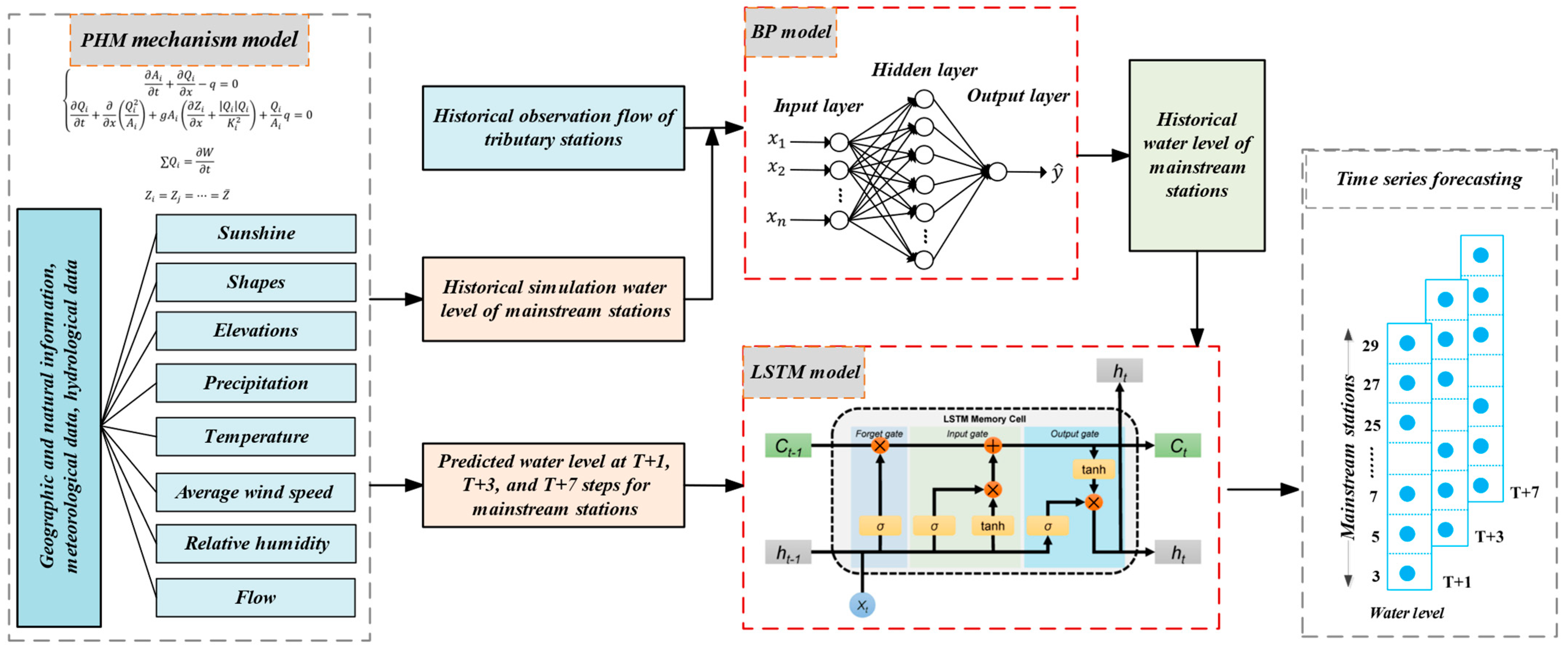
This study established a PHM-BP-LSTM model to forecast the water level in the mainstream of the Yangtze River Three Gorges reservoir basin. The overall development process of the model is presented in Figure 2. Firstly, we established the PHM mechanism model to simulate the water level data of the mainstream stations, which could provide a large amount of simulated water level data for the subsequent deep learning model, thus solving the problem of insufficient data. Subsequently, the BP neural network model was constructed based on historical data from known tributary stations and simulated data from the mechanism model. This model predicted the historical water level data of the mainstream stations, utilizing simulated data from the mechanism model for model training and validation. Next, the LSTM model was established for time series forecasting of the water level at the mainstream stations using the prediction results from the BP network. Simulated data from the mechanism model were utilized for model testing. Finally, the established models were individually evaluated. Using a hybrid model reduced the data requirements for training a deep learning model, as it can use simulated data from the PHM as input. This can address issues with limited or missing historical data, which is often a challenge for purely data-driven models. To facilitate the training of all models, we performed Z-Score normalization on the input data. We used PyTorch’s deep learning framework and Python’s sklearn library. All models were trained using the Adam optimization algorithm [36].

2.3.1. Back Propagation Neural Network

The Back Propagation (BP) neural network is a widely used neural network model that is trained using the error backpropagation algorithm [37]. It has simple learning algorithms and powerful learning capabilities, which enable it to learn and store a great deal of nonlinear mapping relations of the input-output model without disclosing the mathematical equation that describes these relations. Therefore, we used it to model the mainstream-tributary relationships. The BP neural network is a multilayer feedforward network that consists of two main processes: the forward propagation of information and the backward propagation of error [38]. The network comprises three primary layers: the input layer, the hidden layer, and the output layer. Information from external sources is transmitted through the input layer to the network’s hidden layer for processing, and the final result is obtained from the output layer. During training, if the error between the output result of the output layer and the pre-set input value of the BP neural network is large, the network enters the backpropagation stage and updates its weights until the error between the output and the desired result meets certain conditions.

2.3.2. Long Short-Term Memory

The back propagation through time algorithm used in traditional Recurrent Neural Network (RNN) models suffers from the problem of gradient dispersion, especially when dealing with long-term data. This issue leads to slow weight updates, resulting in an inability to effectively capture long-term memory in RNNs [36]. The Long Short-Term Memory (LSTM) network model was proposed to address this challenge. It can remember values over arbitrary intervals, making it well-suited to predict time series given time lags of unknown duration. It is relatively insensitive to gap length and can maintain a stable error gradient across long sequences without suffering from gradient dispersion or explosion. The LSTM model is a particular form of RNN that introduces memory blocks to replace hidden neurons for connecting hidden layers [39]. Each memory block comprises a memory cell (C), an input gate (i), a forget gate (f), and an output gate (o). The LSTM model overcomes the gradient exploding and vanishing issues of conventional RNN by controlling the flow of information between memory cells and gates. The LSTM can learn remote dependencies and effectively capture long-term memory in sequential data by updating or removing previously accumulated information. Its calculation formula is as follows.
i t = σ   W i · h t 1 ,   x t + b i
f t = σ   W f · h t 1 ,   x t + b f
o t = σ   W o · h t 1 ,   x t + b o
C ~ t = t a n h W c · h t 1 ,   x t + b c
C t = f t · C t 1 + i t · C ~ t
h t = o t · tanh ( C t )
where x t represents the input at moment t, h t 1 represents the hidden state at moment t − 1, that is, the output state at the previous time, i t represents the output of the input gate at moment t to control the influence of the input on the internal memory unit, f t represents the output of the forgetting gate at moment t, which controls which information in the memory unit at the previous time needs to be forgotten, o t represents the output of the output gate at moment t, and determines which information needs to be output to the state at the next time, C t represents the state of the internal memory unit at moment t, storing the long-term memory of the network, C ~ t represents the candidate state at moment t and the update information of the internal state at the current time. h t represents the output at moment t, W i , W f , W o , W c represent the weight matrix, b i , b f , b o , b c are the corresponding biases, σ · , t a n h · represents the activation function.

2.4. Comparative Modes

2.4.1. Support Vector Regression

The Support Vector Machine (SVM) regression algorithm is called Support Vector Regression (SVR), which converts nonlinear features into linear features and increases dimensionality using kernel functions [40]. SVR is a supervised learning algorithm that follows the same principle as SVM: finding the best-fitting curve or hyperplane. Generally, SVR follows the structural risk minimization (SRM) theory instead of the empirical risk minimization (ERM) employed by most traditional ANNs. SRM aims to decrease the upper limit of the generalization error, while ERM seeks to reduce the training error. Therefore, the SVR model achieves an optimum network structure and avoids overfitting [41].

2.4.2. Classification and Regression Tree

The Classification and Regression Tree (CART) algorithm partitions a set of samples into two child nodes by identifying one input variable and one break-point [42]. The algorithm begins at the root node, which is the entire set of available training samples. It performs recursive binary partitioning for each node until no further split is possible or a certain termination criterion is satisfied. The best split is identified at each node by an exhaustive search, testing all potential splits on each input variable and break-point. The split corresponding to the minimum deviations is selected by predicting two child nodes of samples with their mean output variables. Typically, an overly large tree is constructed, and pruning is employed to sequentially remove the splits that insufficiently contribute to training accuracy. After constructing a tree, an inquiry sample is assigned to one of the terminal leaves (non-splitting leaf nodes) and is then predicted with the mean output value of the samples belonging to the leaf node [43]. The CART algorithm’s simple structure and good interpretability have made it widely used in practice.

2.5. Model Evaluation Index

To measure the degree of fit between predicted and observed values and to evaluate the performance of the model, the root mean square error (RMSE), mean absolute error (MAE), and goodness of fit (R2) of the model were calculated.
R M S E = 1 n i = 1 n y i y ^ i 2
M A E = 1 n i = 1 n y i y ^ i
R 2 = 1 i = 1 n y i y ^ i 2 i = 1 n y i y ¯ 2
where, n is the number of data, and y ,   y ^ ,   y ¯ are the observed data, predicted data, and mean observed data, respectively.
Model accuracy is measured by the MAE and RMSE, which range between −∞ and +∞ and between 0 and +∞, respectively, and have an ideal value of 0 [44]. The goodness of fit refers to the degree to which the regression line fits the observed values [45]. The statistic that measures goodness of fit is the coefficient of determination R2, which ranges between 0 and 1.

3. Results and Discussion

In this section, we first present the simulation results of the PHM mechanism model. Next, we present and discuss the water level prediction results of the BP neural network and LSTM models. Finally, we compare the performance with other machine learning techniques (SVR and CART models) for different prediction scenarios (T + 1 step, T + 3 step, T + 7 step). We also analyze the advantages and limitations of these techniques in water level prediction.

3.1. Building the Connections between Mainstream and Its Tributaries in TGR

We used the BP neural network to model the mainstream-tributaries relationships in the TGR area. We compared its performance with the mechanism model (PHM) that simulates the water level based on physical equations. Taking the historical hydrological data of the known tributary stations as input and the water level of the mainstream station as the output, we randomly divided the data into a 50% training set and a 50% validation set to train and validate the BP model. Then, we used RMSE, MAE, and R2 as evaluation criteria.
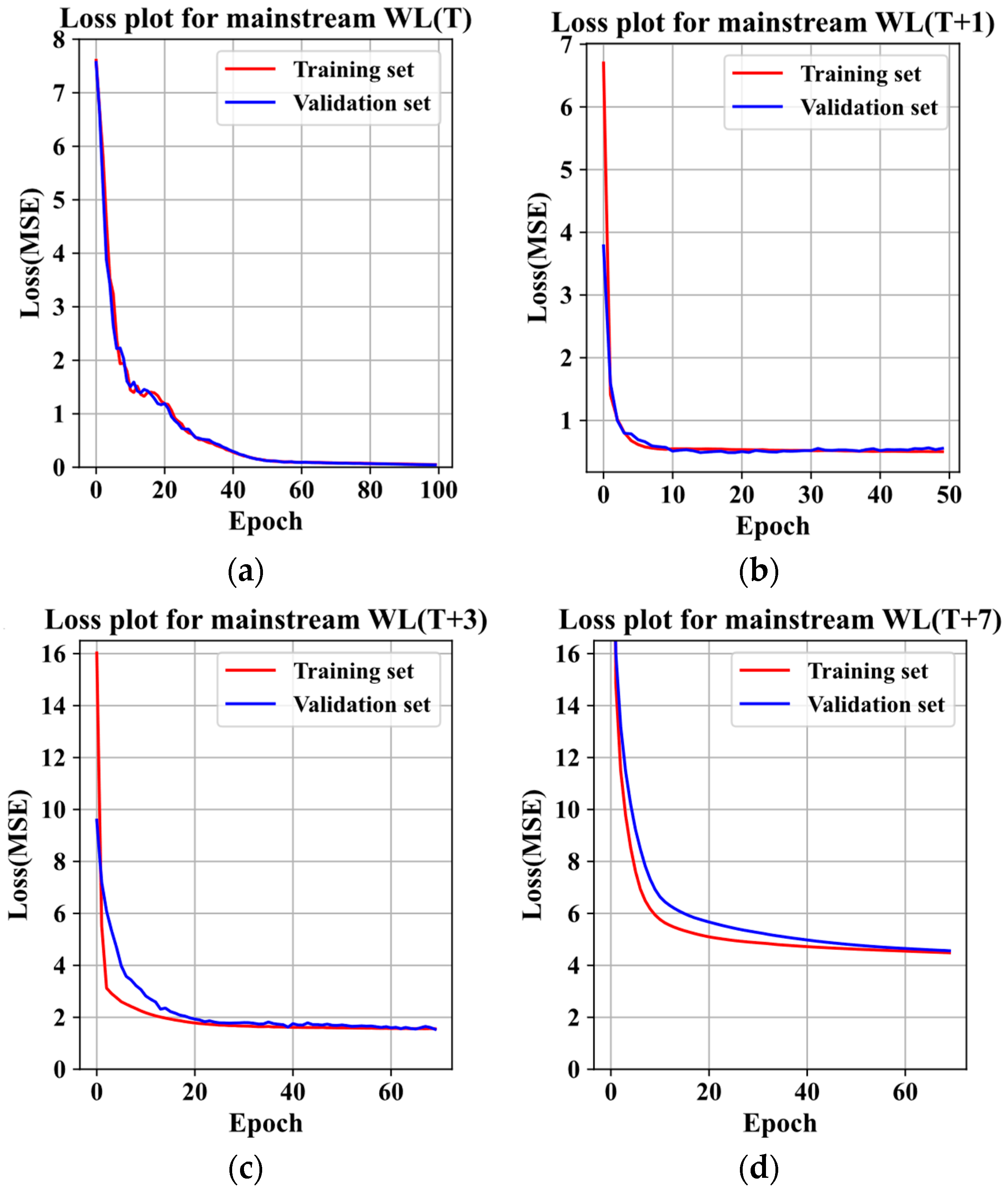
Figure 3 shows the convergence of the mean square error (MSE) for both the training and validation sets of the mainstream water level prediction model. It can be observed that after 100 epochs of training, the MSE values of the training and validation sets tend to stabilize and converge to nearly 0. This indicates that the BP model can effectively learn the inherent relationship between mainstream and tributary water levels and avoid overfitting or underfitting problems.
Table 1 presents the model’s prediction accuracy for each station along the mainstream. As can be seen, the water level prediction model exhibited relatively high accuracy at each mainstream station. The prediction accuracy remained consistently high in both the training and validation sets, with both RMSE and MAE relatively low (on the original data scale), and with an R2 value above 0.9. Within the validation set, the smallest R2 was 0.939 and the largest R2 was 0.999. These results indicate that the BP model can reliably predict the water level of mainstream stations by modeling the mainstream-tributaries relationships.
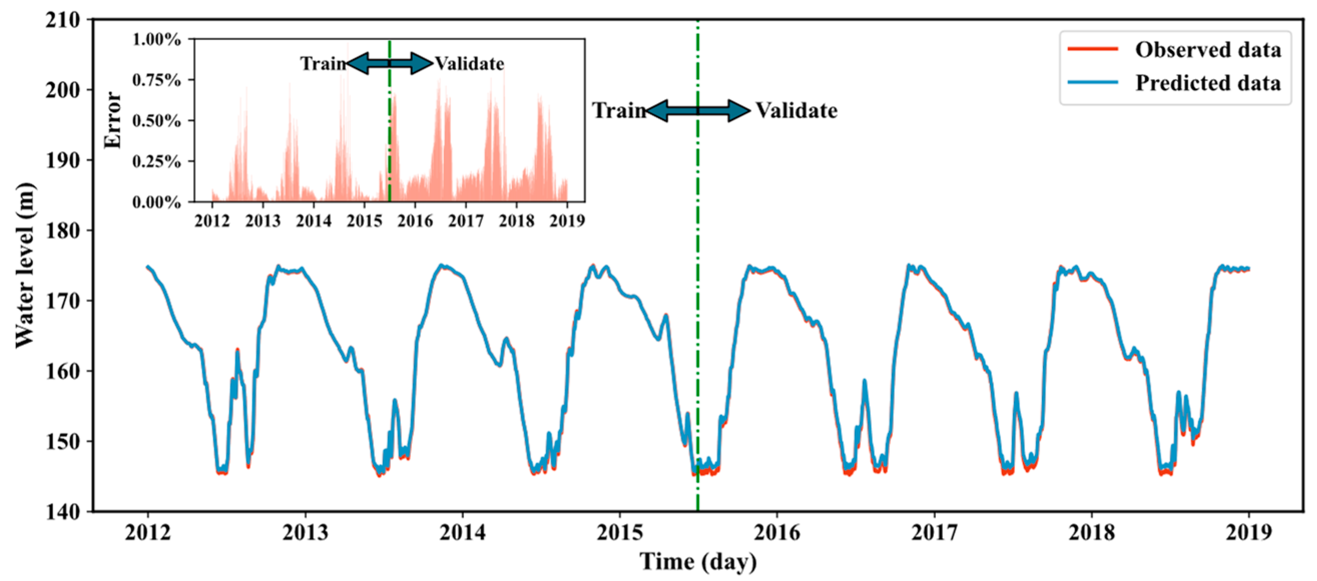
To illustrate the performance of the BP model in predicting the water level changes of the mainstream stations in the TGR area by modeling the mainstream-tributary relationships, we selected the dam-front (No.29 station) water level prediction as an example. As shown in Figure 4, the red line represents the observed values, while the light blue line represents the model-predicted values. The data covers the period from 2012 to 2019, with the first half used for training the model and the last used for validation. The BP model can capture the temporal variation and peak values of the water level very well, and is very close to the observed data. The top-left graph displays the relative error of each sample, which shows that the relative error for both the training and validation sets remained below 1%, indicating that the predictions are highly reliable.
Traditionally, mechanism models simulate the hydrological changes of the mainstream by using the temporal information of multiple tributaries [46,47]. At the same time, machine learning methods are rarely applied to establish the relationship between the mainstream and tributaries. Our study demonstrates that deep learning models are an effective way to build mainstream-tributaries relationships. Our results are consistent with some previous studies. For example, Lallahem et al., (2005) used the BP neural network to simulate water level changes, finding that the BP neural network had high accuracy and stability [48]. Furthermore, our study shows that the BP model can capture the nonlinear relationship between mainstream and tributary water levels and has high prediction accuracy. However, the BP model has limitations in dealing with time series data. It does not have a memory mechanism, which means it cannot capture the long-term dependencies and temporal patterns in the data. Numerous studies reveal that the temporal changes of the mainstream time series require introducing time series forecasting models [49,50].

3.2. Water Level Forecasting Based on the Proposed Model at Different Time Tasks

We applied the LSTM model to predict the time series water level at the mainstream stations. Taking the historical mainstream water level data predicted by the BP neural network as input, and the water level at T + 1, T + 3, or T + 7 steps in each mainstream station as output, we randomly split the data into a 50% training set and a 50% validation set for LSTM training and validation, respectively. Then, we used the data simulated by the mechanism model for each mainstream station to test the LSTM model. Figure 3 shows the convergence of the MSE for the training and validation sets of the LSTM-based mainstream water level time series prediction model (T + 1, T + 3, and T + 7). As shown in Figure 3, after training, the MSE values of both the training and validation sets tended to stabilize, indicating that the LSTM model can effectively predict the time series of water levels and avoid over-fitting or under-fitting problems.
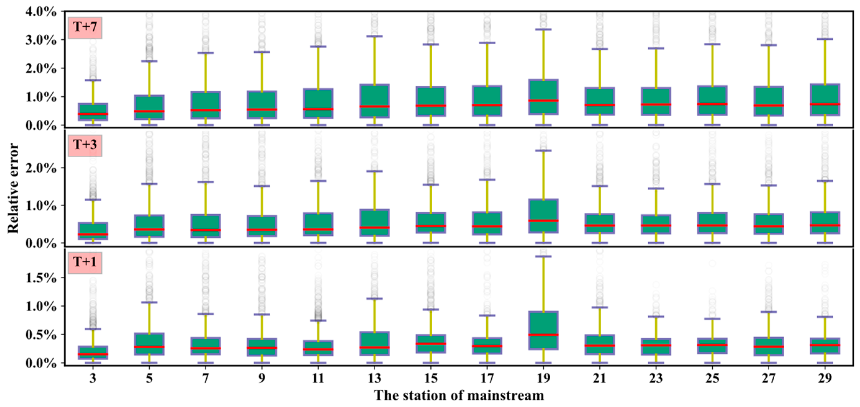
Figure 5 shows the box plots of relative error for each mainstream station at T + 1, T + 3, and T + 7 steps using the LSTM model, which reflect the distribution and degree of dispersion of relative errors between the test set data and the predicted data at each mainstream station. As can be seen, the relative error of all mainstream stations in the time series prediction at T + 1, T + 3, and T + 7 steps is lower than 4%, and the median relative error is lower than 1%. It can also be seen that all mainstream stations have similar relative error ranges at T + 1, T + 3, and T + 7 step predictions, indicating that the LSTM model has relatively average prediction capability for each station in water level prediction tasks at mainstream stations for all steps. Figure 5 also shows that as the prediction steps increase, the relative error ranges also increase but remain at a low level. Therefore, the LSTM model can be considered reliable in time series prediction tasks.
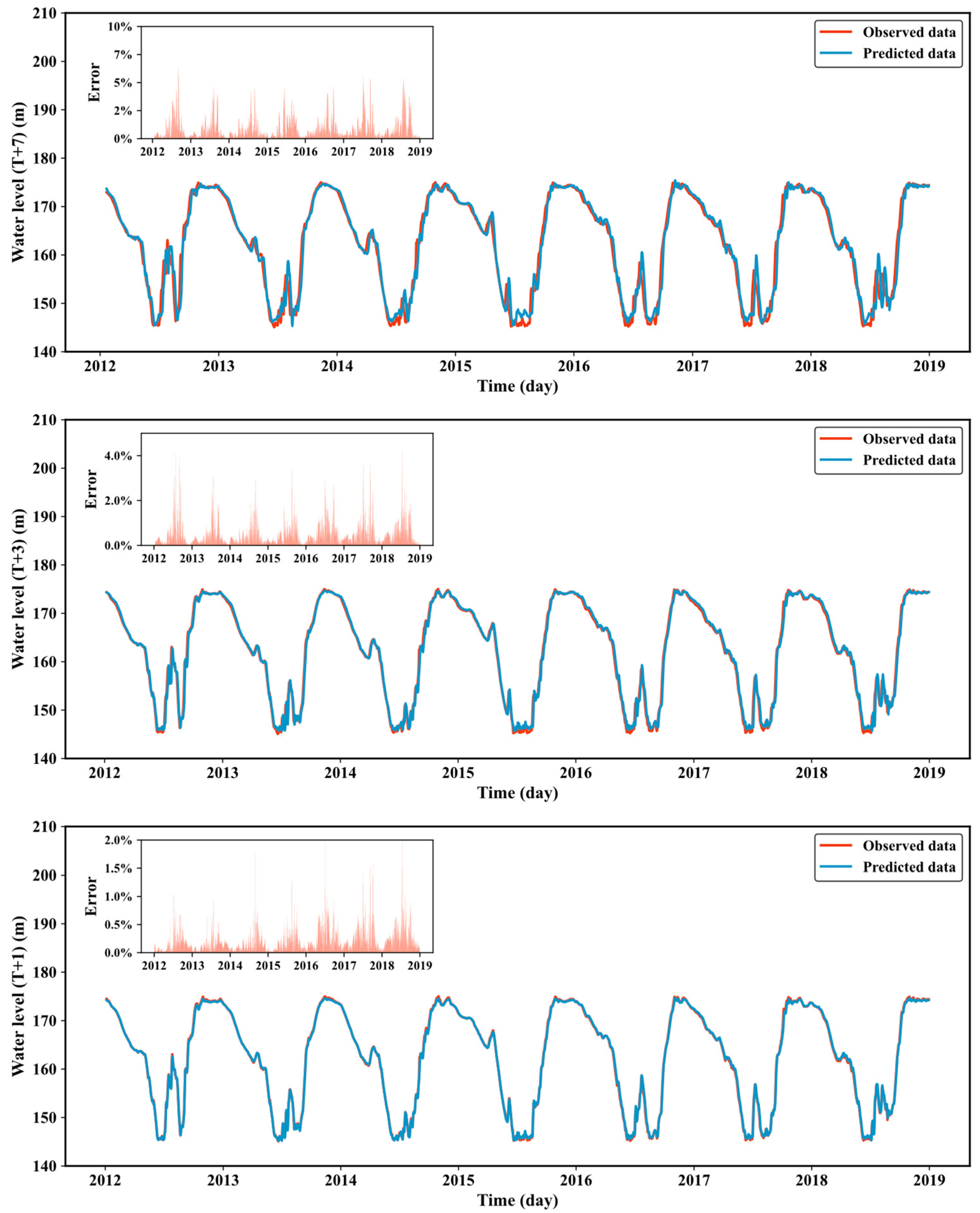
The analysis of the relative error box plots indicates that LSTM has a relatively average prediction capability at each mainstream station. To illustrate the performance of the LSTM model in predicting multi-step (T + 1, T + 3, T + 7) water levels of the mainstream stations in the TGR area, we selected the dam-front (No.29 station) water level prediction as an example. As shown in Figure 6, the red line represents observed values and the light blue line represents predicted values by the LSTM model. The plot in the upper left corner shows the relative error of each sample. The LSTM model can capture temporal variation and peak values of water level very well and is very close to the observed data. Relative errors are smaller for predictions at T + 1, T + 3, and T + 7 steps, indicating reliable predictions and better fitting effects.
Our study confirms that LSTM is an effective way to characterize water level changes, consistent with the findings of Liu et al., (2021), who developed a real-time rolling forecast approach for the short-term water levels of urban inland and external rivers using LSTM, addressing the high uncertainty of river water level prediction in Fuzhou city, China [51]. The results verified the feasibility of LSTM in water level forecasting. In addition, the results show that the PHM-BP-LSTM model can well capture the time-varying and peak water levels, and the model has high accuracy in simulating long-term diurnal water levels. Similarly, the predictive performance of LSTM is affected by the increase in time steps, manifested as a significant increase in model error with the increase in prediction task time. Previous studies have shown that model hyperparameters affect the predictive effect of the model [52]. In this study, we used the Bayesian optimization technique to optimize the hyperparameters [53]. The results of LSTM hyperparameter optimization are shown in Table 2.
Notably, our study develops a multi-site collaborative prediction strategy, which models the spatial relationship between mainstream and tributaries using the BP neural network, and feeds the results into the LSTM to capture the temporal dynamics of the water level time series. In this way, the spatio-temporal correlation of water level changes among different stations is established, and finally, the future water level data of multiple stations are simultaneously output, achieving the goal of multi-site collaborative prediction. The results also confirm the effectiveness of this method for large-scale river water level prediction.

3.3. Model Comparisons with Conventional Machine Learning Approaches

Table 3 presents the accuracy statistics for the LSTM, SVR, and CART models. Regarding RMSE and MAE, the LSTM model showed greater accuracy than the SVR or CART models for all time steps. In contrast, the lowest RMSE- and MAE-based errors were achieved by the LSTM model followed by the SVR and CART models. Therefore, the LSTM model outperformed the SVR and CART models. In forecasting the one-day-ahead water level for TGR, the LSTM model (RMSE = 1.054 m, MAE = 0.489 m) showed the best performance among the developed standalone models, while the CART model (RMSE = 0.89 m, MAE = 0.619 m) showed the poorest performance. In forecasting the three-days-ahead and one-week-ahead water level for TGR, the LSTM model (RMSE = 1.282 m, MAE = 0.833 m and RMSE = 1.981 m, MAE = 1.321 m) demonstrated the best performance among the developed models, while the SVR model (RMSE = 1.39 m, MAE = 0.981 m and RMSE = 2.136 m, MAE = 1.53 m) showed the poorest performance.
Our research results show that LSTM has certain advantages over traditional machine learning models in multi-site and multi-step simultaneous prediction tasks. Similarly, the prediction performance of LSTM, SVR, and CART will also be affected by the increase in time steps, which shows that the model error significantly increases with the increase in the prediction task time, but compared with SVR and CART, the prediction performance of LSTM is always the best. This shows that the PHM-BP-LSTM model proposed in this paper has superior performance in predicting the water level of mainstream stations in the TGR area.
However, in machine learning, different research perspectives and methods have limitations, and our study is no exception. First, our study only used a single feature (i.e., water level) as input data without considering other factors that may affect water level changes, such as rainfall, evaporation, temperature, etc. This may cause the model to ignore some important information or have some biases [54,55]. Second, due to the length of the paper, our study focuses on the difference between traditional machine learning and LSTM methods in water level prediction and does not compare and analyze different deep learning models, which have also been reported in some recent studies [56,57,58]. Furthermore, the key challenge in this paper is how to interpret the processes behind the predictions made by hybrid models. While hybrid models may demonstrate higher accuracy and efficiency in predicting water level fluctuations, they might also exhibit lower interpretability in revealing underlying causal relationships. To address these issues, in future studies, we plan to improve and extend our work from the following aspects:
(1)
Introduce multi-feature data and construct water level prediction models based on multi-input multi-output or multi-task learning techniques;
(2)
Compare different deep learning techniques for water level prediction tasks, and design more suitable deep learning structures for hydrological data characteristics and patterns.
(3)
Investigate the interpretability issues of hybrid models in predicting water level fluctuations in order to reveal underlying causal relationships more effectively.

4. Conclusions

We proposed a hybrid hydrological model (PHM-BP-LSTM) in forecasting the daily water level of the TGR. Firstly, we used the physical-based hydrological model to simulate the water level of 14 stations in the mainstream. Then, the BP neural network model was constructed based on historical data from known tributary stations and simulated data from the mechanism model. Finally, the LSTM model could effectively predict water levels by using historical water level data predicted by BP neural network as input without requiring boundary conditions and operation rules. The results show that our PHM-BP-LSTM model achieved high prediction accuracy and stability in different prediction scenarios (one-day-ahead, three-days-ahead, seven-days-ahead) at 14 mainstream stations, with RMSE values ranging from 0.793 m to 1.918 m, MAE values ranging from 0.489 m to 1.321 m, and the average relative errors at each mainstream station were controlled below 4% in all three forecasting scenarios. The PHM-BP-LSTM model outperformed other machine learning models (SVR and CART) regarding the RMSE and MAE values in all-time series prediction scenarios at all mainstream stations. The PHM-BP-LSTM model could effectively capture the nonlinear and complex relationship between the mainstream and tributary water levels, as well as the temporal dynamics of water level changes. The developed multi-site collaborative forecasting strategy could simultaneously forecast multiple sites along the mainstream of the TGR area. This strategy can effectively utilize the spatio-temporal information of water level data at different locations to improve the prediction performance of large-scale river systems.

Author Contributions

Methodology, M.X., S.Z. and K.S.; validation, M.X., L.W. and B.Y.; investigation, M.X., X.W. and Z.G.; data curation, M.X., S.Z. and K.S.; writing—original draft preparation, M.X., L.W., X.W., B.Y., Z.G. and K.S.; writing—review and editing, M.X., K.S. and M.S.; visualization, M.X.; supervision, K.S. and M.S.; funding acquisition, K.S. and M.S. All authors have read and agreed to the published version of the manuscript.

Funding

This work was supported by the National Natural Science Foundation of China (No. 52379081; 62072429), Chongqing Science and Technology Commission (CSTB2022TIAD-KPX0199; CSTC2020jcyj-msxmX0792). Yunnan Science and Technology Commission (202202AH210006-4). Chongqing Education Commission (HZ2021008). West Light Foundation of The Chinese Academy of Sciences (E1296001). Chongqing Ph.D. Zhitongche Project (No. sl202100000783).

Data Availability Statement

The data presented in this study are available on request from the corresponding authors.

Conflicts of Interest

The authors declare no conflict of interest.

References

  1. Liu, J.G.; Zang, C.F.; Tian, S.Y.; Liu, J.G.; Yang, H.; Jia, S.F.; You, L.Z.; Liu, B.; Zhang, M. Water conservancy projects in China: Achievements, challenges and way forward. Glob. Environ. Chang. Hum. Policy Dimens. 2013, 23, 633–643. [Google Scholar] [CrossRef]
  2. Lopez-Pujol, J.; Ren, M.X. Biodiversity and the Three Gorges Reservoir: A troubled marriage. J. Nat. Hist. 2009, 43, 2765–2786. [Google Scholar] [CrossRef]
  3. Yang, S.L.; Milliman, J.D.; Li, P.; Xu, K. 50,000 dams later: Erosion of the Yangtze River and its delta. Glob. Planet. Chang. 2011, 75, 14–20. [Google Scholar] [CrossRef]
  4. Ahmed, S.S.; Bali, R.; Khan, H.; Mohamed, H.I.; Sharma, S.K. Improved water resource management framework for water sustainability and security. Environ. Res. 2021, 201, 111527. [Google Scholar] [CrossRef] [PubMed]
  5. Moisello, U.; Todeschini, S.; Vullo, F. The effects of water management on annual maximum floods of Lake Como and River Adda at Lecco (Italy). Civ. Eng. Environ. Syst. 2013, 30, 56–71. [Google Scholar] [CrossRef]
  6. Bengtsson, L.; Malm, J. Using rainfall-runoff modeling to interpret lake level data. J. Paleolimnol. 1997, 18, 235–248. [Google Scholar] [CrossRef]
  7. Kadioglu, M.; Sen, Z.; Batur, E. Cumulative Departures Model for Lake-Water Fluctuations. J. Hydrol. Eng. 1999, 4, 245–250. [Google Scholar] [CrossRef]
  8. Izady, A.; Davary, K.; Alizadeh, A.; Ziaei, A.N.; Alipoor, A.; Joodavi, A.; Brusseau, M.L. A framework toward developing a groundwater conceptual model. Arab. J. Geosci. 2014, 7, 3611–3631. [Google Scholar] [CrossRef]
  9. Irvine, K.N.; Eberhardt, A.J. Multiplicative, Seasonal Arima Models for Lake Erie and Lake-Ontario Water Levels. Water Resour. Bull. 1992, 28, 385–396. [Google Scholar] [CrossRef]
  10. Kasiviswanathan, K.; Saravanan, S.; Balamurugan, M.; Saravanan, K. Genetic programming based monthly groundwater level forecast models with uncertainty quantification. Model. Earth Syst. Environ. 2016, 2, 27. [Google Scholar] [CrossRef]
  11. Wang, K.; Hu, T.F.; Zhang, P.P.; Huang, W.Q.; Mao, J.Q.; Xu, Y.F.; Shi, Y. Improving Lake Level Prediction by Embedding Support Vector Regression in a Data Assimilation Framework. Water 2022, 14, 3718. [Google Scholar] [CrossRef]
  12. Moghaddam, D.D.; Rahmati, O.; Haghizadeh, A.; Kalantari, Z. A Modeling Comparison of Groundwater Potential Mapping in a Mountain Bedrock Aquifer: QUEST, GARP, and RF Models. Water 2020, 12, 679. [Google Scholar] [CrossRef]
  13. Adnan, R.M.; Mostafa, R.R.; Kisi, O.; Yaseen, Z.M.; Shahid, S.; Zounemat-Kermani, M. Improving streamflow prediction using a new hybrid ELM model combined with hybrid particle swarm optimization and grey wolf optimization. Knowl. Based Syst. 2021, 230, 107379. [Google Scholar] [CrossRef]
  14. Adnan, R.M.; Kisi, O.; Mostafa, R.R.; Ahmed, A.N.; El-Shafie, A. The potential of a novel support vector machine trained with modified mayfly optimization algorithm for streamflow prediction. Hydrol. Sci. J. 2022, 67, 161–174. [Google Scholar] [CrossRef]
  15. Ikram, R.M.A.; Ewees, A.A.; Parmar, K.S.; Yaseen, Z.M.; Shahid, S.; Kisi, O. The viability of extended marine predators algorithm-based artificial neural networks for streamflow prediction. Appl. Soft Comput. 2022, 131, 109739. [Google Scholar] [CrossRef]
  16. Rogers, L.L.; Dowla, F.U. Optimization of Groundwater Remediation Using Artificial Neural Networks with Parallel Solute Transport Modeling. Water Resour. Res. 1994, 30, 457–481. [Google Scholar] [CrossRef]
  17. Zhang, Y.C.; Le, J.; Liao, X.B.; Zheng, F.; Li, Y.H. A novel combination forecasting model for wind power integrating least square support vector machine, deep belief network, singular spectrum analysis and locality-sensitive hashing. Energy 2019, 168, 558–572. [Google Scholar] [CrossRef]
  18. Smys, S.; Basar, A.; Wang, H. CNN based flood management system with IoT sensors and cloud data. J. Artif. Intell. 2020, 2, 194–200. [Google Scholar]
  19. Kimura, N.; Yoshinaga, I.; Sekijima, K.; Azechi, I.; Baba, D. Convolutional Neural Network Coupled with a Transfer-Learning Approach for Time-Series Flood Predictions. Water 2020, 12, 96. [Google Scholar] [CrossRef]
  20. Palmitessa, R.; Mikkelsen, P.S.; Borup, M.; Law, A.W.K. Soft sensing of water depth in combined sewers using LSTM neural networks with missing observations. J. Hydro-Environ. Res. 2021, 38, 106–116. [Google Scholar] [CrossRef]
  21. Ikram, R.M.A.; Mostafa, R.R.; Chen, Z.; Parmar, K.S.; Kisi, O.; Zounemat-Kermani, M. Water temperature prediction using improved deep learning methods through reptile search algorithm and weighted mean of vectors optimizer. J. Mar. Sci. Eng. 2023, 11, 259. [Google Scholar] [CrossRef]
  22. Yang, X.Y.; Zhang, Z.R. A CNN-LSTM Model Based on a Meta-Learning Algorithm to Predict Groundwater Level in the Middle and Lower Reaches of the Heihe River, China. Water 2022, 14, 2377. [Google Scholar] [CrossRef]
  23. Baek, S.S.; Pyo, J.; Chun, J.A. Prediction of Water Level and Water Quality Using a CNN-LSTM Combined Deep Learning Approach. Water 2020, 12, 3399. [Google Scholar] [CrossRef]
  24. Yang, S.; Yang, D.; Chen, J.; Santisirisomboon, J.; Lu, W.; Zhao, B. A physical process and machine learning combined hydrological model for daily streamflow simulations of large watersheds with limited observation data. J. Hydrol. 2020, 590, 125206. [Google Scholar] [CrossRef]
  25. Li, G.; Zhu, H.; Jian, H.; Zha, W.; Wang, J.; Shu, Z.; Yao, S.; Han, H. A combined hydrodynamic model and deep learning method to predict water level in ungauged rivers. J. Hydrol. 2023, 625, 130025. [Google Scholar] [CrossRef]
  26. Yuan, Z.; Liu, J.; Liu, Y.; Zhang, Q.; Li, Y.; Li, Z. A two-stage modelling method for multi-station daily water level prediction. Environ. Model. Softw. 2022, 156, 105468. [Google Scholar] [CrossRef]
  27. Lafaysse, M.; Hingray, B.; Etchevers, P.; Martin, E.; Obled, C. Influence of spatial discretization, underground water storage and glacier melt on a physically-based hydrological model of the Upper Durance River basin. J. Hydrol. 2011, 403, 116–129. [Google Scholar] [CrossRef]
  28. Saber, M.; Hamaguchi, T.; Kojiri, T.; Tanaka, K.; Sumi, T. A physically based distributed hydrological model of wadi system to simulate flash floods in arid regions. Arab. J. Geosci. 2015, 8, 143–160. [Google Scholar] [CrossRef]
  29. Li, B.; Yang, G.S.; Wan, R.R.; Dai, X.; Zhang, Y.H. Comparison of random forests and other statistical methods for the prediction of lake water level: A case study of the Poyang Lake in China. Hydrol. Res. 2016, 47, 69–83. [Google Scholar] [CrossRef]
  30. Pan, M.Y.; Zhou, H.N.; Cao, J.Y.; Liu, Y.S.; Hao, J.L.; Li, S.X.; Chen, C.H. Water Level Prediction Model Based on GRU and CNN. IEEE Access 2020, 8, 60090–60100. [Google Scholar] [CrossRef]
  31. Gao, Q.F.; He, G.J.; Fang, H.W.; Bai, S.; Huang, L. Numerical simulation of water age and its potential effects on the water quality in Xiangxi Bay of Three Gorges Reservoir. J. Hydrol. 2018, 566, 484–499. [Google Scholar] [CrossRef]
  32. Li, X.; Sha, J.; Wang, Z.L. Influence of the Three Gorges Reservoir on climate drought in the Yangtze River Basin. Environ. Sci. Pollut. Res. 2021, 28, 29755–29772. [Google Scholar] [CrossRef] [PubMed]
  33. Peel, M.C.; Blöschl, G. Hydrological modelling in a changing world. Prog. Phys. Geogr. 2011, 35, 249–261. [Google Scholar] [CrossRef]
  34. Yang, L.; Zeng, S.; Xia, J.; Wang, Y.; Huang, R.; Chen, M. Effects of the Three Gorges Dam on the downstream streamflow based on a large-scale hydrological and hydrodynamics coupled model. J. Hydrol. Reg. Stud. 2022, 40, 101039. [Google Scholar] [CrossRef]
  35. Zeng, S.; Liu, X.; Xia, J.; Du, H.; Chen, M.; Huang, R. Evaluating the hydrological effects of the Three Gorges Reservoir based on a large-scale coupled hydrological-hydrodynamic-dam operation model. J. Geogr. Sci. 2023, 33, 999–1022. [Google Scholar] [CrossRef]
  36. Singarimbun, R.N. Adaptive Moment Estimation To Minimize Square Error In Backpropagation Algorithm. Data Sci. J. Comput. Appl. Inform. 2020, 4, 27–46. [Google Scholar] [CrossRef]
  37. Robert, H.-N. Theory of the backpropagation neural network. IEEE Xplore 1989, 1, 593–605. [Google Scholar]
  38. Buscema, M. Back propagation neural networks. Subst. Use Misuse 1998, 33, 233–270. [Google Scholar] [CrossRef] [PubMed]
  39. Hochreiter, S.; Schmidhuber, J. Long short-term memory. Neural Comput. 1997, 9, 1735–1780. [Google Scholar] [CrossRef] [PubMed]
  40. Huang, H.; Feng, X.a.; Zhou, S.; Jiang, J.; Chen, H.; Li, Y.; Li, C. A new fruit fly optimization algorithm enhanced support vector machine for diagnosis of breast cancer based on high-level features. BMC Bioinform. 2019, 20, 290. [Google Scholar] [CrossRef]
  41. Lin, J.-Y.; Cheng, C.-T.; Chau, K.-W. Using support vector machines for long-term discharge prediction. Hydrol. Sci. J. 2006, 51, 599–612. [Google Scholar] [CrossRef]
  42. Timofeev, R. Classification and Regression Trees (CART) Theory and Applications; Humboldt University: Berlin, Germany, 2004; p. 54. [Google Scholar]
  43. Morgan, J. Classification and Regression Tree Analysis; Boston University: Boston, MA, USA, 2014; p. 298. [Google Scholar]
  44. Ahmadisharaf, E.; Camacho, R.A.; Zhang, H.X.; Hantush, M.M.; Mohamoud, Y.M. Calibration and validation of watershed models and advances in uncertainty analysis in TMDL studies. J. Hydrol. Eng. 2019, 24, 03119001. [Google Scholar] [CrossRef]
  45. Legates, D.R.; McCabe, G.J., Jr. Evaluating the use of “goodness-of-fit” measures in hydrologic and hydroclimatic model validation. Water Resour. Res. 1999, 35, 233–241. [Google Scholar] [CrossRef]
  46. Ramkar, P.; Yadav, S. Identification of critical watershed using hydrological model and drought indices: A case study of upper Girna, Maharashtra, India. ISH J. Hydraul. Eng. 2021, 27, 471–482. [Google Scholar] [CrossRef]
  47. Tang, J.; Yin, X.-A.; Yang, P.; Yang, Z. Assessment of contributions of climatic variation and human activities to streamflow changes in the Lancang River, China. Water Resour. Manag. 2014, 28, 2953–2966. [Google Scholar] [CrossRef]
  48. Lallahem, S.; Mania, J.; Hani, A.; Najjar, Y. On the use of neural networks to evaluate groundwater levels in fractured media. J. Hydrol. 2005, 307, 92–111. [Google Scholar] [CrossRef]
  49. Aminikhanghahi, S.; Cook, D.J. A survey of methods for time series change point detection. Knowl. Inf. Syst. 2017, 51, 339–367. [Google Scholar] [CrossRef]
  50. Montanez, G.; Amizadeh, S.; Laptev, N. Inertial hidden markov models: Modeling change in multivariate time series. In Proceedings of the AAAI Conference on Artificial Intelligence, Austin, TX, USA, 25–30 January 2015; Volume 29. [Google Scholar]
  51. Liu, Y.; Wang, H.; Feng, W.W.; Huang, H.C. Short Term Real-Time Rolling Forecast of Urban River Water Levels Based on LSTM: A Case Study in Fuzhou City, China. Int. J. Environ. Res. Public Health 2021, 18, 9287. [Google Scholar] [CrossRef]
  52. Hutter, F.; Hoos, H.; Leyton-Brown, K. An efficient approach for assessing hyperparameter importance. In Proceedings of the 31st International Conference on Machine Learning, Beijing, China, 21–26 June 2014; pp. 754–762. [Google Scholar]
  53. Wu, J.; Chen, X.-Y.; Zhang, H.; Xiong, L.-D.; Lei, H.; Deng, S.-H. Hyperparameter optimization for machine learning models based on Bayesian optimization. J. Electron. Sci. Technol. 2019, 17, 26–40. [Google Scholar]
  54. Shan, K.; Song, L.; Chen, W.; Li, L.; Liu, L.; Wu, Y.; Jia, Y.; Zhou, Q.; Peng, L. Analysis of environmental drivers influencing interspecific variations and associations among bloom-forming cyanobacteria in large, shallow eutrophic lakes. Harmful Algae 2019, 84, 84–94. [Google Scholar] [CrossRef]
  55. Yaseen, Z.M.; Allawi, M.F.; Yousif, A.A.; Jaafar, O.; Hamzah, F.M.; El-Shafie, A. Non-tuned machine learning approach for hydrological time series forecasting. Neural Comput. Appl. 2018, 30, 1479–1491. [Google Scholar] [CrossRef]
  56. Barzegar, R.; Aalami, M.T.; Adamowski, J. Short-term water quality variable prediction using a hybrid CNN–LSTM deep learning model. Stoch. Environ. Res. Risk Assess. 2020, 34, 415–433. [Google Scholar] [CrossRef]
  57. Mohammed, S.J.; Zubaidi, S.L.; Ortega-Martorell, S.; Al-Ansari, N.; Ethaib, S.; Hashim, K. Application of hybrid machine learning models and data pre-processing to predict water level of watersheds: Recent trends and future perspective. Cogent Eng. 2022, 9, 2143051. [Google Scholar] [CrossRef]
  58. Morovati, K.; Nakhaei, P.; Tian, F.; Tudaji, M.; Hou, S. A Machine learning framework to predict reverse flow and water level: A case study of Tonle Sap Lake. J. Hydrol. 2021, 603, 127168. [Google Scholar] [CrossRef]
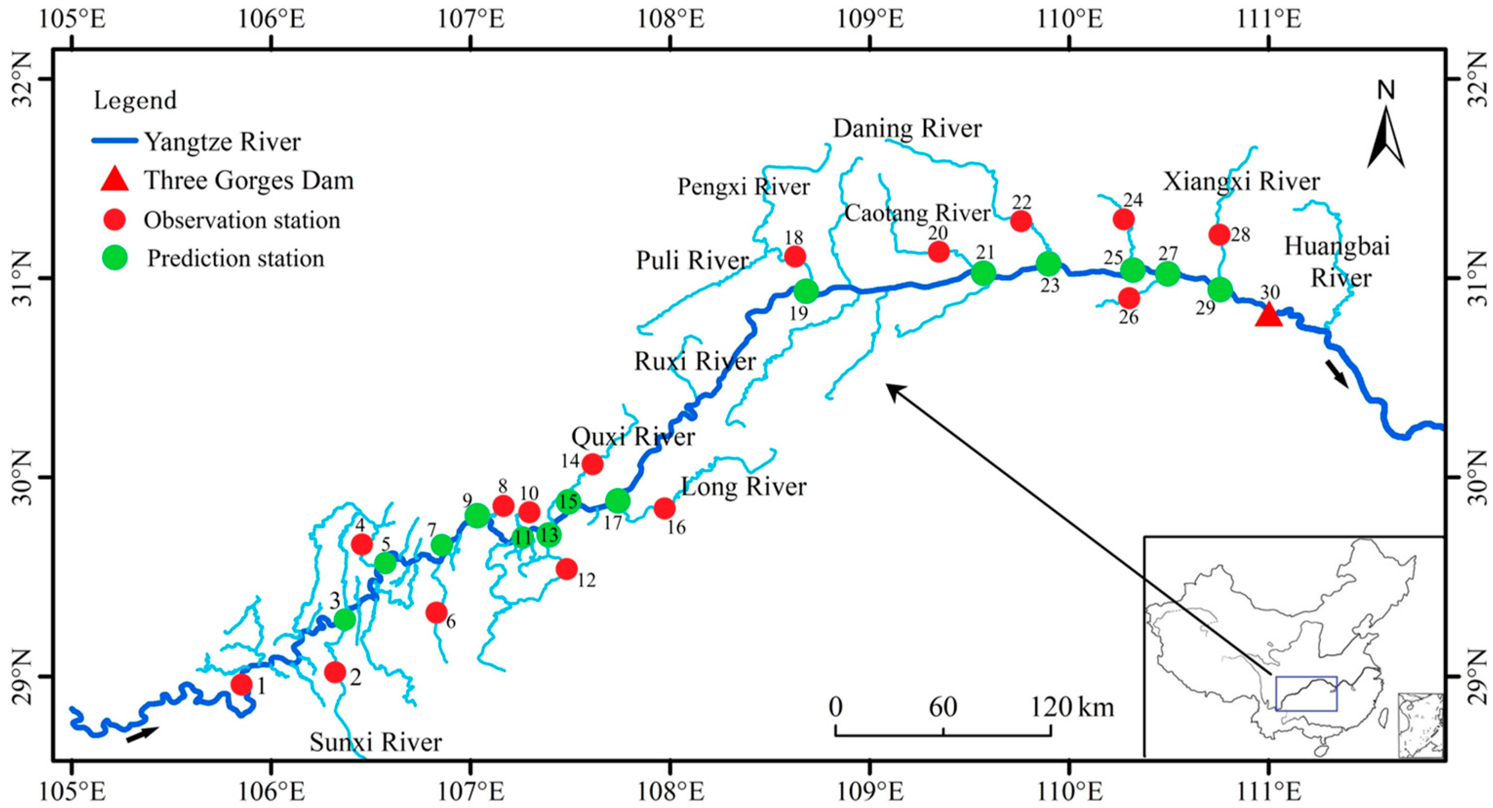
Figure 1. Overview of the study area in the Three Gorges Reservoir (TGR), China. The numbers adjacent to the dots denote the positional indices of the stations. The red circular dots represent observation stations with historically observed flow data (day). The red triangle represents the Three Gorges Dam, which has historically observed water level data (day). The green circular dots represent the junctures of mainstream and tributary. These dots serve as simulated locations and represent the positions that necessitate prediction. The black arrows represent the flow direction.
Water 15 03191 g001
Figure 2. The building process of the proposed model (PHM-BP-LSTM). The arrows points towards the direction of data generation from PHM and subsequent deep learning analysis.
Water 15 03191 g002
Figure 3. (a) Loss plot for BP model for predicting water level (T) of mainstream stations. (bd) Loss plot for LSTM model for predicting multi-step (T + 1, T + 3, T + 7) water level (WL) of mainstream stations.
Water 15 03191 g003
Figure 4. The fitting effect of the prediction (predicted data) dam-front (No.29 station) water level and the simulated water level (observed data) of the mechanism model. The inner plot represents the relative error after taking the absolute value.
Water 15 03191 g004
Figure 5. Box plots for the absolute value of the relative error between the water level predicted by the LSTM multi-step model and the simulated value of the mechanism model (the station of the mainstream is shown as the green dots in Figure 1).
Water 15 03191 g005
Figure 6. The fitting effect of the multi-step (T + 1, T + 3, T + 7) time series prediction (predicted data) water level of the dam-front (No. 29 station) and the simulated water level (observed data) of the mechanism model. The inner plot represents the relative error after taking the absolute value.
Water 15 03191 g006
Table 1. Performance of BP model in forecasting historical water levels of mainstream stations (the location index of mainstream stations is shown as the green dots in Figure 1).
Location
Index
Training SetValidation Set
RMSEMAER2RMSEMAER2
30.8830.4140.9180.6610.3630.939
50.8180.5260.9660.6840.4530.969
70.3550.2390.9950.3110.2180.996
90.3610.2710.9960.3210.2460.997
110.6480.5040.9920.6130.4920.994
130.7510.4590.9920.7630.4970.993
151.0250.6860.9850.8830.5910.991
170.4460.2960.9970.4870.3210.997
191.4530.9390.9741.2750.8450.984
210.7730.480.9930.6640.4090.995
230.4120.2720.9980.3810.2680.998
250.2320.1420.9990.2560.1630.999
270.6390.3920.9950.5610.3470.997
290.2410.1530.9990.2590.1740.999
Table 2. The hyperparameters of the LSTM model for different prediction steps.
StepTime LagHidden SizeLearning RateNum LayersBatch SizeActivation Function
T + 14320.001132relu
T + 318320.001132relu
T + 730320.0005132relu
Table 3. Performance of the models in multi-step time series forecasting water levels of mainstream stations. Δ represents the increase in RMSE and MAE of SVR and CART compared to LSTM, and—represents the performance decline of SVR and CART compared with LSTM.
StepModelTraining SetValidation Set
RMSE MAE RMSE MAE
T + 1LSTM0.717-0.412 0.793 0.489
SVR0.783(−Δ9.2%)0.524(−Δ27.2%)0.858(−Δ8.1%)0.598(−Δ22.3%)
CART0.764(−Δ6.6%)0.503(−Δ22.1%)0.89(−Δ12.2%)0.619(−Δ26.6%)
T + 3LSTM1.23-0.71 1.282 0.833
SVR1.377(−Δ11.9%)0.923(−Δ30%)1.39(−Δ8.4%)0.981(−Δ17.8%)
CART1.237(−Δ0.6%)0.781(−Δ10%)1.379(−Δ7.6%)0.94(−Δ12.8%)
T + 7LSTM1.909-1.168 1.981-1.321-
SVR2.132(−Δ11.7%)1.443(−Δ23.5%)2.136(−Δ7.8%)1.53(−Δ15.8%)
CART2.008(−Δ5.2%)1.333(−Δ14.1%)2.118(−Δ6.9%)1.437(−Δ8.8%)
Disclaimer/Publisher’s Note: The statements, opinions and data contained in all publications are solely those of the individual author(s) and contributor(s) and not of MDPI and/or the editor(s). MDPI and/or the editor(s) disclaim responsibility for any injury to people or property resulting from any ideas, methods, instructions or products referred to in the content.