Article

Exploring the Effect of Meteorological Factors on Predicting Hourly Water Levels Based on CEEMDAN and LSTM

1
School of Hydraulic and Ecological Engineering, Nanchang Institute of Technology, Nanchang 330099, China
2
Jiangxi Provincial Technology Innovation Center for Ecological Water Engineering in Poyang Lake Basin, Nanchang 330029, China
*
Author to whom correspondence should be addressed.
Water 2023, 15(18), 3190; https://doi.org/10.3390/w15183190
Submission received: 3 August 2023 / Revised: 1 September 2023 / Accepted: 4 September 2023 / Published: 7 September 2023

Abstract

:
The magnitude of tidal energy depends on changes in ocean water levels, and by accurately predicting water level changes, tidal power plants can be effectively helped to plan and optimize the timing of power generation to maximize energy harvesting efficiency. The time-dependent nature of water level changes results in water level data being of the time-series type and is essential for both short- and long-term forecasting. Real-time water level information is essential for studying tidal power, and the National Oceanic and Atmospheric Administration (NOAA) has real-time water level information, making the NOAA data useful for such studies. In this paper, long short-term memory (LSTM) and its variants, stack long short-term memory (StackLSTM) and bi-directional long short-term memory (BiLSTM), are used to predict water levels at three sites and compared with classical machine learning algorithms, e.g., support vector machine (SVM), random forest (RF), extreme gradient boosting (XGBoost), and light gradient boosting machine (LightGBM). This study aims to investigate the effects of wind speed (WS), wind direction (WD), gusts (WG), air temperature (AT), and atmospheric pressure (Baro) on predicting hourly water levels (WL). The results show that the highest coefficient of determination ( R 2 ) was obtained at all meteorological factors when used as inputs, except at the La Jolla site. (Burlington station ( R 2 ) = 0.721, Kahului station ( R 2 ) = 0.852). In the final part of this article, the complete ensemble empirical mode decomposition adaptive noise (CEEMDAN) algorithm was introduced into various models, and the results showed a significant improvement in predicting water levels at each site. Among them, the CEEMDAN-BiLSTM algorithm performed the best, with an average RMSE of 0.0759 m h 1 for the prediction of three sites. This indicates that applying the CEEMDAN algorithm to deep learning has a more stable predictive performance for water level forecasting in different regions.

1. Introduction

In order to mitigate the issues arising from the extensive consumption of fossil fuels and the resulting climate and environmental changes, people have increasingly embraced the utilization of renewable resources such as solar and wind energy. However, these resources are susceptible to the impacts of weather changes, leading to unpredictable challenges. In comparison, tidal power generation appears more dependable due to its predictability [1]. In [2], it is mentioned that tidal range devices, which utilize the difference in water level between high and low tide, can generate energy for power generation. From the perspective of new energy development needs, new energy generation is a meaningful project. Based on the design of tidal power generation devices, real-time prediction of water level can better utilize tidal energy as well as lay the foundation for optimizing tidal power generation devices.
With the development of artificial intelligence, many researchers now use artificial intelligence algorithms to predict water levels. Khan et al. conducted a long-term prediction of lake water levels by SVM, and the authors experimentally concluded that SVM has more accurate prediction accuracy than multilayer perceptron (MLP) and a conventional multiplicative seasonal autoregressive model (SAR) [3]. Many researchers use ANN in predicting water levels [4,5,6,7] and use extreme learning machines (ELMs) compared with artificial neural networks (ANNs). They found that ELMs are more stable and accurate in predicting water levels. However, due to the increase in data volume, classical machine learning algorithms cannot fit their target features well [8]. In previous research, many scholars have attempted to employ deep learning techniques for the prediction of water levels [9,10,11].
Deep learning includes many kinds of algorithms, among which the classical models are recurrent neural network (RNN) [12], gate recurrent unit (GRU) [13], and LSTM [14]. These models excel in handling larger volumes and prediction tasks, especially the LSTM, and this algorithm performs better for long-term prediction tasks. GRU is able to learn the water level trend, and the convolutional neural network (CNN) learns the spatial correlation between water level data observed at neighboring water stations to predict the water level at multiple stations with a CNN-GRU model [15]. Assem et al. conducted tests using a deep CNN model at three stations along the Shannon River. The results demonstrate that this model outperforms four well-known time series prediction models [10]. In addition to the above, some researchers have used CNN and LSTM to combine water quality and water level applications, and it has been demonstrated that CNN-LSTM performs better in predicting the water level [16].
Nonetheless, the interaction between water levels and weather conditions has been explored in various studies. For example, Zan et al. investigated the impact of changes in Poyang Lake’s water level and area on weather patterns. They observed that as the water level and area increase, there is a reduction in the lake’s latent heat flux (LH), wind speed, and vapor flux over the lake [17]. Behzad et al. used support vector machines (SVMs) and artificial neural networks (ANNs) to predict their groundwater levels and compared the accuracy of the two models by different time scales [18]. Choi et al. evaluated the accuracy of decision tree (DT), RF, and artificial neural network (ANN) models for predicting water levels by using daily water meter data from 2009 to 2015 as dependent variables and meteorological data and upstream water level as independent variables [19]. Arkian et al. investigated the effects of precipitation, wind speed, temperature, and number of sunsets on the water level of Lake Urmia, where a reduced wind speed may affect the evaporation process of Lake Urmia’s water body, leading to a decrease in water level [20]. Attempts to explore the relationship between climatic factors and water level are a possible point of exploration. Cox et al. further improved the neural network approach by incorporating meteorological factors of wind and wind direction into the model, significantly improving the short-term prediction of wind and water level [21]. Furthermore, forecasting fluctuations in lake levels to sustain the ecology of HoB is of the utmost importance. Yadav et al. utilized daily lake levels and additional meteorological data as inputs for the wavelet–support vector machine (WA-SVM), resulting in optimal model outcomes. This approach was subsequently extended to achieve compelling lake-level predictions with impressive results [22]. Many past studies have emphasized the link between weather elements and water levels. However, a more thorough exploration is necessary. As data pile up, traditional machine learning models might struggle with predictions. Therefore, using deep learning to examine the intricate meteorological–water level relationship becomes a valuable experiment.
From the above review, it can be seen that many researchers use ANNs, SVM, ELMs, and some deep learning models for predicting water levels. Moreover, Stack-LSTM, BiLSTM, and LSTM can also be used for the prediction of water levels, for example, by investigating the impact of meteorological factors on the prediction of water levels in deep learning and assessing the stability and accuracy of such models. In addition, there are few studies related to the influence of water level and meteorological factors based on deep learning as a way of analyzing the relationship between meteorological factors and the water level, which is also to be analyzed and studied. In addition to deep attitude learning, this paper also tried XGB and LightGBM models to compare with deep learning; the reason why these two gradient-related models are used is that these models are better for nonlinear capture ability. Then, they are compared with the more frequently used SVM and RF. Furthermore, Lu et al. added the CEEMDAN algorithm for short-term water quality prediction through decision tree-based XGBoost and RF models, and the results showed that both CEEMDAN-RF and CEEMDAN-XGBoost had higher predictability than the other models [23]. The application of the CEEMDAN algorithm for the prediction of water levels is a method worth exploring.
The objectives of this study were to (1) investigate the effects of meteorological factors on the predicted water levels through different water levels and multiple meteorological factor combination input strategies; (2) develop hour-by-hour water level prediction models for LSTM, Stack-LSTM, Bi-LSTM, SVM, RF, XGB, and LightGBM using limited meteorological and water level data; (3) explore the seasonal effects on predicting water levels based on the optimal meteorological and water level combinations from (1) and (2); (4) employ CEEMDAN to decompose the raw data and use the decomposed features as inputs for various models, comparing the accuracy of these models in water level prediction, using the optimal meteorological and water level combinations from (1) and (2); (5) explore the predictive accuracy of LightGBM compared to other models; (6) compare the predictive performance of machine learning models and deep learning models for time series forecasting tasks.

2. Materials and Methods

2.1. Study Area Description

In this study, three stations with complete water level and meteorological data, namely Burlington, La Jolla, and Kahului, were selected from the topographic maps of the National Oceanic and Atmospheric Administration (NOAA) Tide and Current Data website (https://tidesandcurrents.noaa.gov/map/, accessed on 14 July 2023), with specific site locations shown in Figure 1.

2.2. Data Collection and Analysis

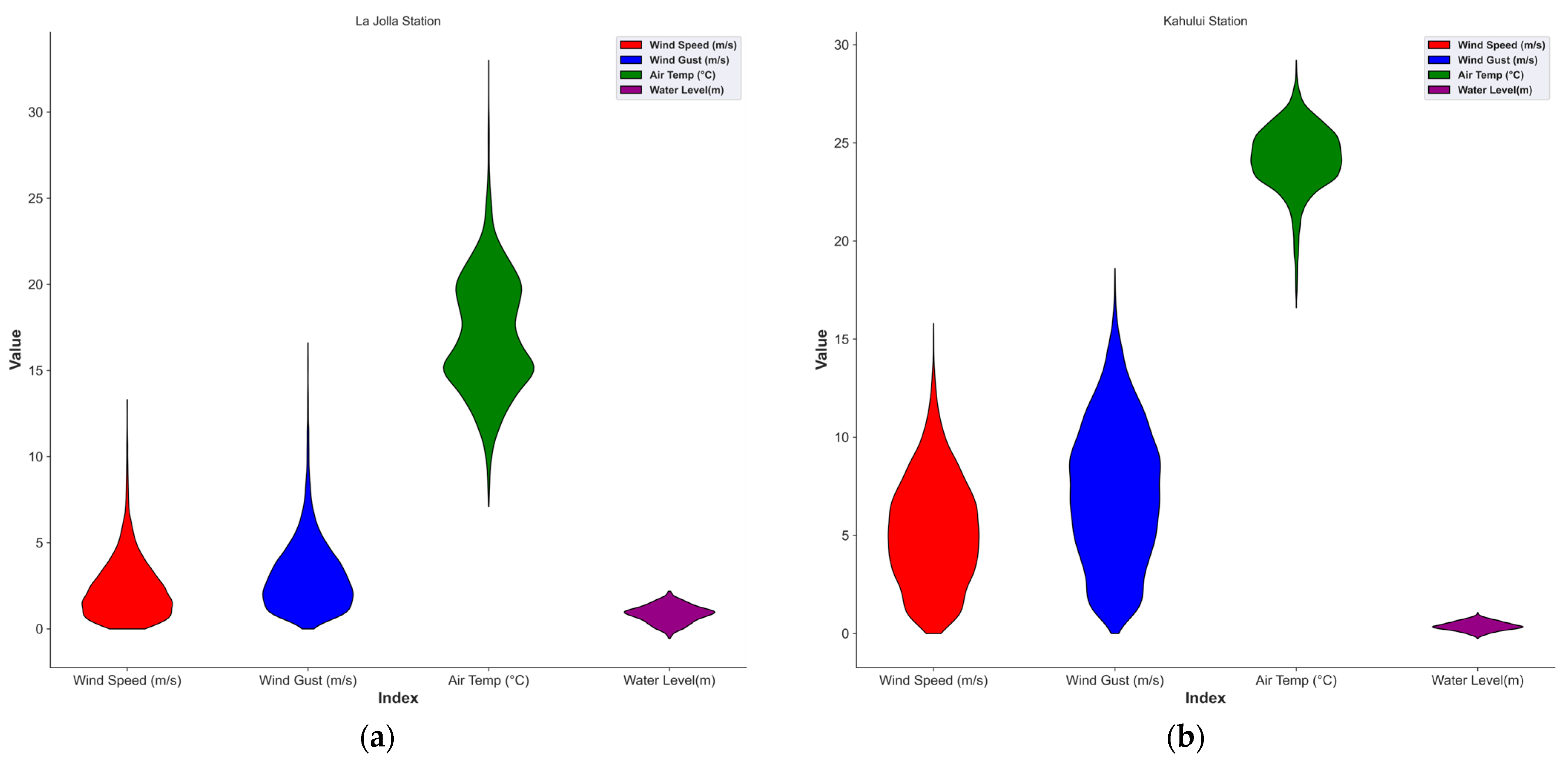
Data were collected for the three different stations, hour-by-hour water levels from January 2022 to January 2023 and the corresponding meteorological data for each station, Wind Speed (WS) ( m / s ), Wind Gust (WG) ( m / s ), Air Temp (AT) ( ° C ), and Barometric Pressure (Baro) ( m b ), and detailed data descriptions of the Water Level (WL) and weather stations ( m ) studied are shown in Table 1. Due to the enormous magnitude of WD and Baro, a detailed description of the statistics for each site is given in Table 2. In contrast, a violin visualization of the WS, WG, AT, and WL data is given in Figure 2. Data for this paper were obtained from NOAA water level meteorological monitoring stations; NOAA data have provided the scientific database for many researchers, for example, the green vegetation fraction of Gutman et al. was derived using NOAA/AVHRR data and was used in numerical weather models [24]. Gruber et al. obtained estimates of the Earth’s total longwave radiation from NOAA’s satellite data, summarized the changes in satellite instruments through these data, and provided the algorithms used by NOAA in obtaining the longwave radiation dataset [25]. As shown above, the data from the NOAA site are reliable and experimental.

2.3. Machine Learning Algorithms for Predicting Water Level References

2.3.1. Support Vector Machine (SVM)

The SVM algorithm is a supervised learning machine learning algorithm for pattern recognition and data analysis developed by Cortes et al. [26]. It has been widely used for regression analysis and prediction in agriculture, meteorology, environmental science, chemical elemental analysis, biomedicine [27], and other related research fields. Based on the structural risk minimization (SRM) principle, SVMs seek to minimize upper bounds on the generalization error rather than on the empirical error, and SVMs models generate regression functions by applying a set of high-latitude linear functions [28]. We refer to the computational idea of the nonlinear classification task mentioned in [29]. The specific mathematical expression formula of SVM is reviewed:
f x = s i g n k = 1 N α k y k ψ x , x k + b )
Given a training set y k , x k k = 1 N consisting of N data samples, where x k R n is the k th input pattern and y k R n is the k th output, where α k are positive real constants and b is a real constant. For the kernel function of SVM mainly controlled by ψ x , x k , which is divided into linear polynomial kernel function (Poly), radial basis kernel function (RBF), the RBF kernel function used in this lab: ψ x , x k = e x p x x k 2 2 σ , where σ and k are constants.

2.3.2. Random Forest (RF)

The RF model was proposed by Breiman et al. [30]. The unique key point is the idea of “Bagging”, as the random forest is composed of multiple decision trees, which are controlled by the variance. RF models have been widely used in prediction and regression analysis tasks. Random forests, which can naturally accommodate feature selection and interactions in learning, have unique advantages in dealing with small samples, high-dimensional feature spaces, and complex data [31]. The RF mentioned in [32] is referenced and the mathematical expression of RF:
T j = i = 1 n g j X i j s Y i
where s Y i R is set as a precondition, Y i 1,2 , 3 , , k and denotes the oridinal reponse of observation i with convariates X i j . j = 1,2 , 3 , , p , and then the test statistic is used to test the relationship between the ordinal response and the predictor variable X j ; where g j :   X j R p j is a non-random transformation of the predictor variable X j from a one-dimensional space vector to a pj-dimensional vector space. For a more detailed explanation of the RF definition, see [32].

2.3.3. Extreme Gradient Boosting (XGBoost)

The XGBoost algorithm was proposed by Chen et al. (2016) [33], and is an algorithm or engineering implementation based on GBDT. The basic idea of XGBoost is the same as GBDT, but with some optimizations, such as second-order derivatives to make the loss function more accurate; regular terms to avoid tree overfitting; block storage to allow parallel computation, etc. XGBoost is an efficient distributed implementation that allows for fast training. Since XGBoost uses an additive learning scheme with a second-order approximation, its second-order derivative is a second-order approximation. The input is denoted as x i , and the output as y i . The mathematical expression for XGBoost in the actual training is as follows [34]:
L t = i = 1 n l y i , z i t 1 + f t x i + Ω f t
Equation (1) is a regularized objective, l ( · , · ) denotes the loss between the objective y i and the prediction z i , and Ω ( · ) denotes the complexity of the model, the tree is fitted in an additive manner with z i ( t ) = z i ( t 1 ) + f t x i , and t represents the t -th iteration of the training process.

2.3.4. Light Gradient Boosting Machine (LightGBM)

LightGBM is a machine learning algorithm similar to XGBoost proposed by Ke et al. to implement gradient boosting decision trees, which are not satisfactorily efficient and scalable when the feature dimension is high, and the data size is large at XGBoost [35]. LightGBM possesses two special techniques, gradient-based one-side sampling (GOSS) and exclusive feature bundling (EFB). With the addition of these two techniques, LightGBM performs more than 20 times faster than the traditional GBDT implementation algorithm on multiple public datasets and achieves almost the same status in terms of accuracy. For the algorithm details, please see [35]. LightGBM uses GOSS to determine the splitting point by calculating the variance gain, ranking the samples by the absolute value of the gradient, and taking the top a × 100% of the data samples in terms of gradient value called A. Then, a subset B of size b × A c is randomly selected from the retained sample A c . Finally, the splitting is performed by the estimated variance V j ( d ) on A B [36].
V j d = 1 n x i A l g i + 1 a b x i B l g i 2 n l j d + x i A r g i + 1 a b x i B r g i 2 n r j d  
where A l = x i A : x i , j d ; A r = x i A : x i , j > d ; B l = x i B : x i , j d ; B r = x i B : x i , j > d ; g i denotes the negative gradient of the loss function; and 1 a b is used to normalize the sum of the gradients.

2.4. Deep Learning Algorithms for Predicting Water Level Reference

2.4.1. Long Short-Term Memory (LSTM)

Deep learning is a machine learning concept based on ANN, which in principle belongs to a sub-branch of machine learning. Deep learning models outperform shallow machine learning models and traditional methods of data analysis [37]. The LSTM is a complex RNN model proposed by Hochreiter et al. [14]. The LSTM solves the problem of gradient disappearance and gradient explosion of RNN for time series task prediction [37]. LSTM is different from RNN in the design of its hidden layer, whose basic unit is a memory block containing multiple memory cells and three adaptive multiplication control gates. The core of each memory cell is a self-connected linear cell called the constant error disk (CEC) [38]. The LSTM is mainly based on multiplying the input of the cell with the activation function of the input gate, then selectively forgetting the information in the cell state through the forgetting gate, and finally multiplying the activation with the output gate to obtain the next state value. The mathematical description of the LSTM model is as follows [39]:
f t = σ w f h t 1 , x t + b f
i t = σ w i h t 1 , x t + b i
C t ˜ = t a n h w c h t 1 , x t + b c
O t = σ w o h t 1 , x t + b o
C t = f t C t 1 + C t ˜ i t
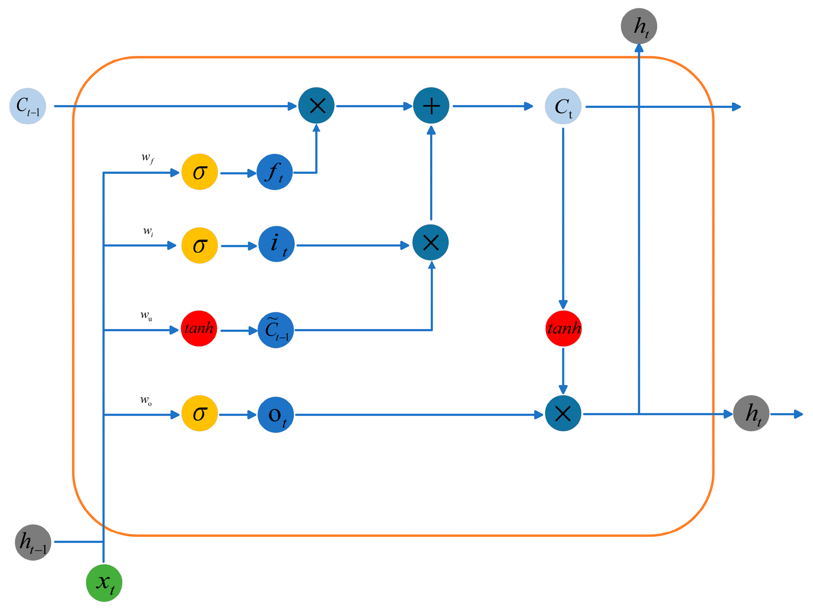
w f , w i , w c , and w o represent the weight matrices of the forgetting gate, input gate, update unit, and output gate, respectively, and b f , b i , b c , and b o epresent the bias terms in each of their equations, respectively. σ is the function of the sigmoid activation function in the LSTM, and tanh is the activation function in the update unit. The main difference between t a n h and the other three activation functions is the value range, sigmoid is [0,1], and t a n h is [−1,1], both used to control each link’s output. The basic cell structure of LSTM is shown in Figure 3.

2.4.2. Stack Long Short-Term Memory (StackLSTM)

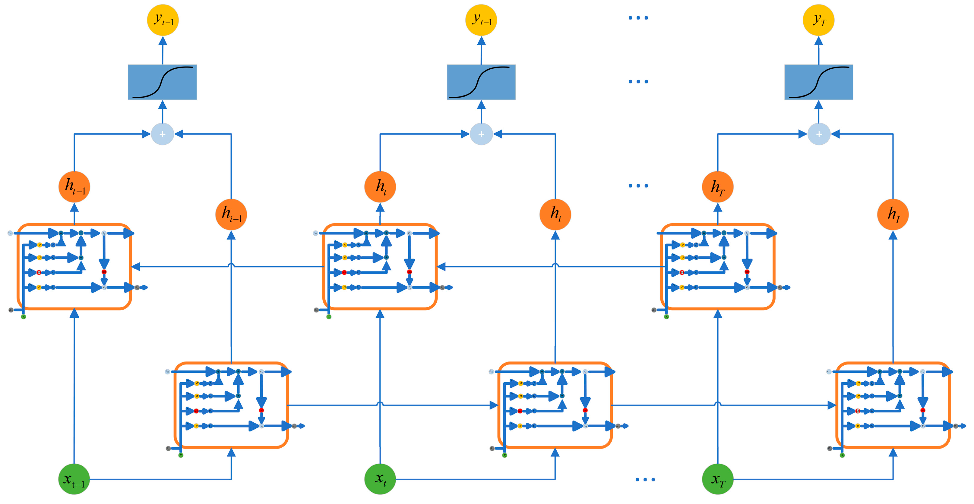
While the traditional LSTM models the time series in left-to-right order, the stackLSTM augments the traditional LSTM by borrowing a stack pointer. The current position determines which cell in the LSTM can provide C t . In addition to adding elements to the end of the time series, StackLSTM provides a pop-up operation that moves the stack pointer to the previous element [40]. StackLSTM achieves more excellent operability for time-series data manipulation through stack structure and operations such as popping and inserting. The stacked LSTM is structured as a multi-layer LSTM, which stacks multiple LSTMs together, and in some cases, its results are better than the LSTM. However, it should be noted that this also increases the complexity of the model. Pattana-Anake et al. (2022) found that the two-layer LSTM stacking approach gives good results in experiments [41]. This paper uses the stacking approach with only two LSTM layers [41]; the basic structure of StackLSTM is shown in Figure 4.

2.4.3. Bi-Directional Long Short-Term Memory (BiLSTM)

A bidirectional recurrent neural network (BRNN) is proposed by Schuster et al. [42], which can be trained only in the future frame of the predefined future frame without the restriction of using input information, and is implemented by simultaneous training in the positive and negative directions; good results are obtained in the experiments [42]. LSTM is a complex RNN model. BiLSTM can obtain both past and future information in many sequential tasks where this processing structure is needed. In contrast, the hidden state h t in LSTM cannot obtain future information. The basic idea of BiLSTM is that the forward and backward of each sequence are two independent hidden states, which are used to obtain the past and future information, respectively, and finally the two hidden states are summed to obtain the final output [43]. The hidden layers of each layer and the final output can be expressed as [44]:
h t = L S T M x t , h t 1
h i = L S T M x t , h i 1
y t = σ α t h t + β t h i + C t
where the L S T M · represents its standard model; meanwhile, α t and β t denote the hidden layer of forward and backward output weights, respectively; and C t is the bias optimization parameter of the hidden layer at time t . The typical structure of the BiLSTM is shown in Figure 5.

2.5. Input Portfolio Strategy

Many researchers have explored studies on variable input strategies. Cui et al. verified the stability of the proposed model via reducing the number of variable pairs [45]. Fan et al. verified the accuracy and stability of the model using different combinations of inputs [46]. In this study, the effects of different meteorological factors on predicted water levels were assessed based on different combinations: based on existing data, different combinations of meteorological conditions and water levels are used as inputs for the model. These combinations are as follows: (1) wind speed (WS), wind direction (WD), wind gust (WG), air temperature (AT), barometric pressure (Baro), and water level (WL) are all taken as factors for predicting water level using all available meteorological features; (2) WS, WD, WG, and WL are taken as factors for predicting water level, focusing on meteorological features related to wind; (3) AT, Baro, and WL are factors for predicting water levels using two air-related meteorological features; and (4) WL, WS, and AT are investigated as factors for predicting water level, examining the impact of selecting one relevant factor each from wind- and air-related features; more detailed combinations of inputs are shown in Table 3. In this paper, we trained the model by using the samples from the previous moment as training data and the data from the next moment as labels. The ratio of the training set to the test set is 8:2. The running environment of this paper is Python. Regarding deep learning, TensorFlow is used as the base framework for LSTM, and all experiments are performed on the CPU without GPU acceleration.

2.6. Complete Ensemble Empirical Mode Decomposition Adaptive Noise (CEEMDAN)

EMD, EEMD, CEEMD, and wavelet decomposition are noise analysis methods. CEEMDAN is an improved algorithm based on EEMD [47]. For the EMD algorithm to decompose the signal, there are modal aliasing problems. The EEMD and CEEMD decomposition algorithms mitigate the modal aliasing problem of EMD decomposition by adding positive and negative Gaussian white noise to the signal to be decomposed. EMD and CEEMD can decompose the original signal into high-frequency signals called intrinsic modes functions (IMFs) in many iterations. However, these two algorithms decompose the signal to obtain the intrinsic modal components, which always leave a certain amount of white noise, affecting the subsequent processing and analysis of the signal. In order to solve this problem, Torres et al. proposed a new signal decomposition algorithm as CEEMDAN [48]. The implementation process of CEEMDAN can be given as follows:
(1). White noise ω i ( t ) with a noise standard deviation of ε is added to the original signal X i ( t ) , which can be expressed by the following equation:
X i ( t ) = X ( t ) + ε 0 ω i ( t ) , i = 1 , 2 , , k
where k is denoted as a real number.
(2). An E M D decomposition operation is performed on the set of signals, and then the components of each decomposition are averaged.
I M F 1 ¯ ( t ) = K 1 i = 1 K I M F 1 i ( t )
(3). Calculate the residuals of the first stage.
r 1 ( t ) = X ( t ) I M F 1 ¯ ( t )
(4). The signal r 1 t + ε 1 E M D 1 ( ω i ( n ) ) is further E M D -decomposed, and the second IMF mode is calculated.
I M F 2 ¯ ( t ) = K 1 i = 1 K E M D 1 ( r 1 ( t ) + ε 1 E M D 1 ( ω i ( t ) ) )
where E M D k ( · ) denotes the k t h   I M F mode decomposed by the E M D algorithm.
(5). In the succeeding stage, the k + 1 t h component and the k t h residual are calculated, and the specific equation can be described as follows:
I M F k + 1 ¯ ( t ) = K 1 i = 1 K E M D 1 ( r k ( t ) + ε k E M D k ( ω i ( t ) ) )
r k ( t ) = r k 1 ( t ) I M F k ¯ ( t )
(6). Repeat Equations (17) and (18) until the residual component ( r k ) no longer satisfies the decomposition condition and the decomposition stops. Finally, the original signal R can be expressed as the following equation.
X ( t ) = i = 1 K I M F i ¯ ( t ) + R ( t )
where R ( t ) is final residual.
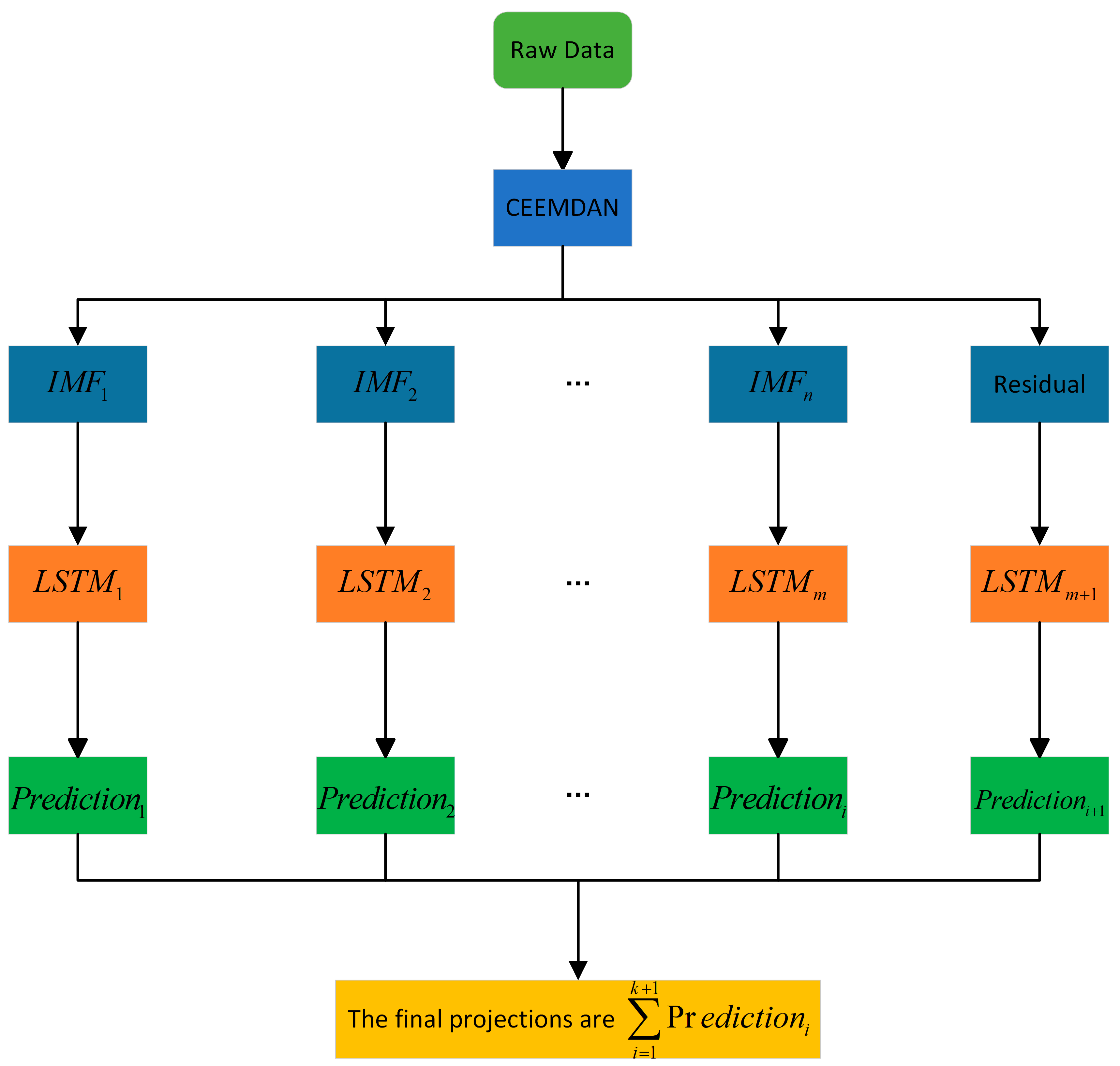
CEEMDAN is used for data decomposition and denoising, noise decomposition and denoising, and the process of applying it to each model based on it is essential. Figure 6 gives the detailed workflow of CEEMDAN.

2.7. Model Comparison Statistical Analysis

The accuracy and performance of the study model in predicting hourly water levels were statistically determined using two commonly used estimation methods, decision coefficient ( R 2 ), root mean square error ( R M S E ), and a combination of mean absolute error ( M A E ) and normalized root mean square error ( n R M S E ) indicators were evaluated and compared. The mathematical expression equations were as follows:
R 2 = i = 1 n Y i , o Y i , p 2 i = 1 n Y i , o Y ¯ i , o 2
R M S E = 1 n i = 1 n Y i , o Y i , p 2
M A E = 1 n i = 1 n Y i , o Y i , p
n R M S E = 1 n i = 1 n Y i , o Y i , p 2 Y i , o ¯
where Y i , o , Y i , p , Y ¯ i , p , Y i , o ¯ and n are the observed values, predicted values, mean of observed values, mean of predicted values, and total number of samples, respectively. A higher R 2 represents a higher precision ranging from 0 to 1. When it is infinitely close to 1, the data are very well-fitted. Conversely, lower R M S E , M A E , and n R M S E represent better performance of the model.
For the model requirements in this study, the original meteorological data and water level data were normalized to the maximum and minimum values ( M a x M i n ), limited to between 0 and 1, and then put into each model for training, normalized using the following formula:
x n = x i x m i n x m a x x m i n
where x n and x i represent the moralized and original training and test sets, respectively; x m a x and x m i n are the maximum and minimum values in the test and training sets.

2.8. Hyperparameter Tuning

In this study, no optimization method was used to set the parameters of the model. For the deep learning-based LSTM parameters, the parameters of the LSTM and its variants of the model were adjusted based on the data of the Burlington site. In order to validate the model’s universality to the same problem, this parameter was carried over to the individual models of the other two sites. Through several validations, the radial basis function (RBF) nonlinear kernel function was finally chosen to be used as its parameter in SVM. The same number of decision trees (N_Estimators: 50) was used for RF and XGB. For LightGBM, the parameters were determined by several adjustments, as shown in Table 4. In the models based on deep learning LSTM and its variants, the number of neurons was uniformly set to 200. The activation function was set to a linear rectifier function (ReLU), which introduces a nonlinear property to help the model learn complex data relationships. The optimizer used Adam to train the model, while the mean squared error (MSE) loss function is used to measure the gap between the predicted and actual values of the model. Epochs are the number of iterations, and batch size is the data in each batch during training. The final learning rate is set to the default value with better prediction results through several trial calculations. The specific parameters are shown in Table 4.

3. Results

3.1. Compare the Accuracy of Each Model Prediction for Different Combinations of Inputs

See Table 5, Table 6 and Table 7 for the hourly water level statistical results predicted by Burlington, Kahului, and La Jolla, three deep learning models, and four machine learning models. These tables list the statistical results of SVM, RF, XGBoost, LightGBM, LSTM, StackLSTM, and BiLSTM models tested with four combinations of inputs.
As shown in Table 5, the models have significant differences in predicting water levels in different areas under different combinations. Taking Burlington as an example, the performance of each model is analyzed in detail. Compared with SVM, RF, and XGB, models based on LSTM show better performance with the highest R 2 , lowest R M S E , M A E , and n R M S E , and the prediction accuracy in the order of magnitude is StackLSTM, BiLSTM, and LightGBM, SVM, RF, and XGBoost. In terms of input strategy, the highest progress was obtained in predicting water levels when all meteorological factors, WS, WD, WG, AT, Baro, and WL, were used as inputs, followed by WS, WD, WG, and WL combined inputs, AT, Baro, and WL combined inputs, and finally WS, AT, and WL combined inputs. From the experimental results, it is concluded that when more meteorological factors are used, it is more accurate for predicting water levels.
As shown in Table 6, it has similar and identical prediction results to Table 5. The best results were obtained for the water level prediction at the Kahului site when all meteorological factors plus water level were used as inputs, with an R 2 of 0.85 higher than the minimum prediction accuracy of 0.018. For the combination of WS, WD, WG, and WL inputs, the value of R 2 was 0.847, and the value of R M S E was 0.093 m h 1 , which were also more satisfactory results. Using only WS, AT, and WL for the combination, we obtained R 2 values of 0.852 and M A E and R M S E values of 0.072 m h 1 and 0.091 m h 1 , respectively, which were the lowest among all predictions. These good prediction results were obtained based on the LSTM model and its variants based on Santo learning, and these results demonstrate the great potential of deep learning-based LSTM and its variants for hour-by-hour water level prediction.
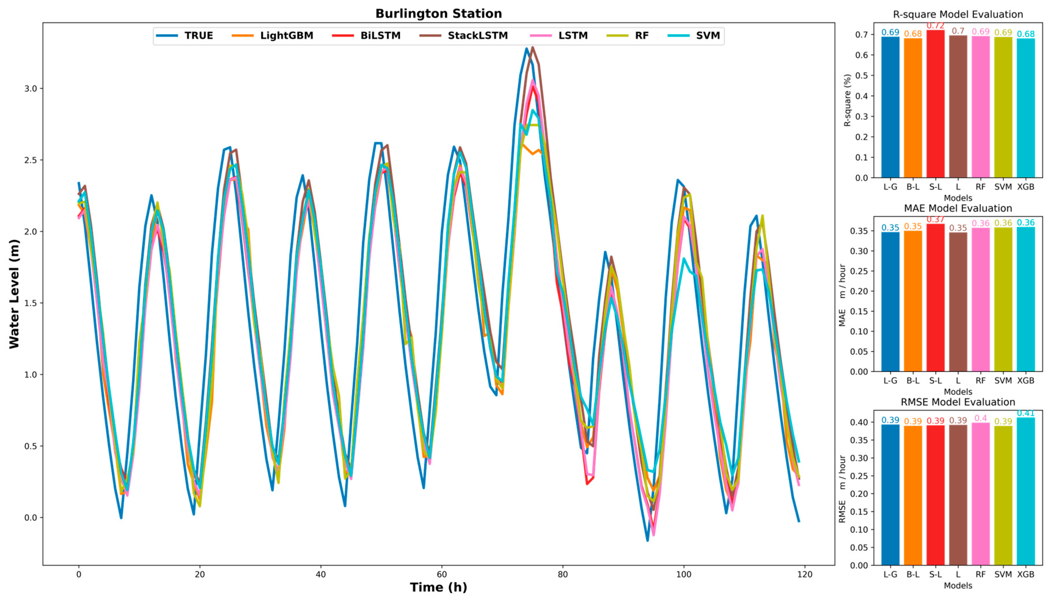
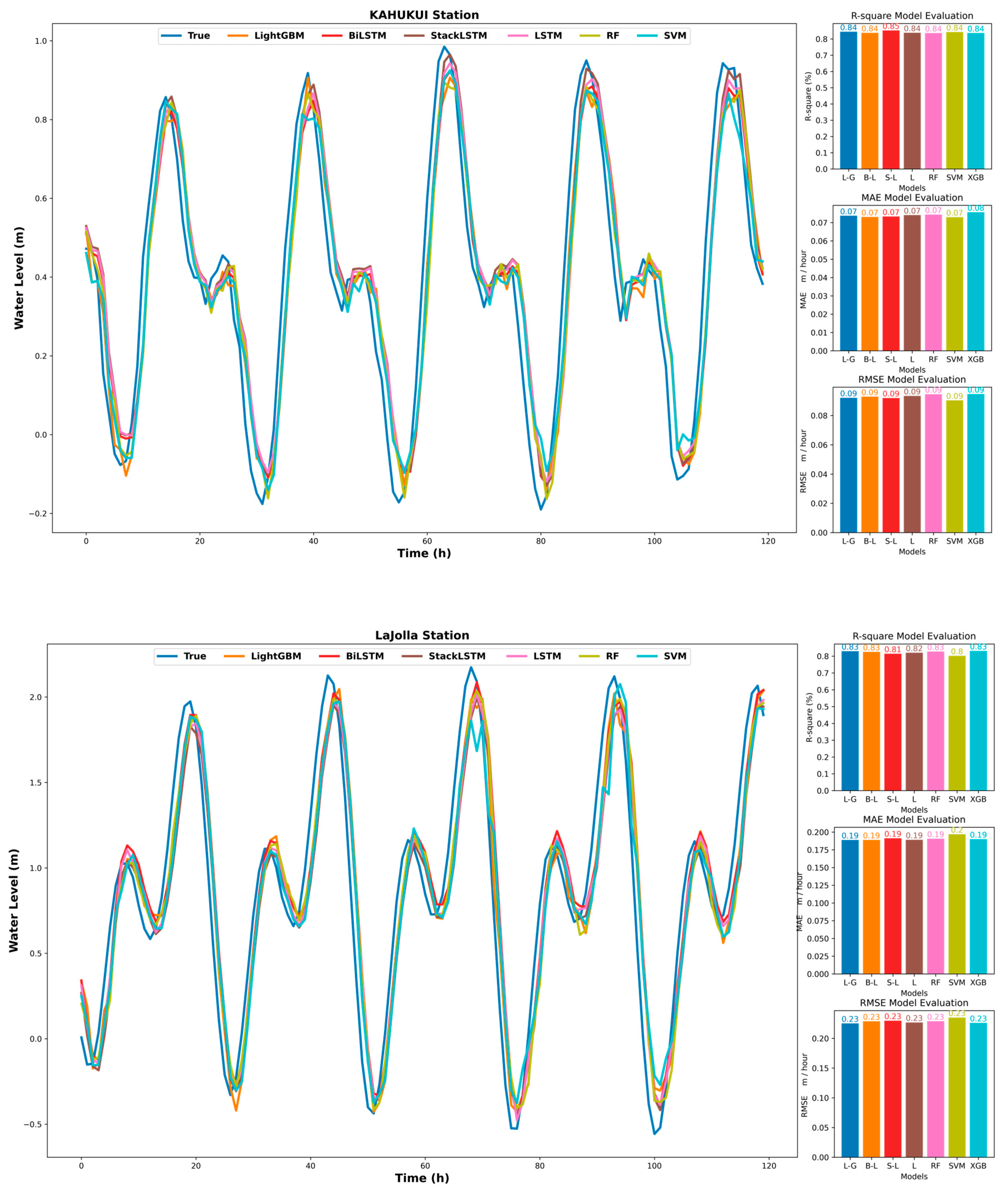
Using all climate factors as input, the results are visually interpreted by prediction curves, as shown in Figure 7 which reveals the prediction effect of each model more clearly. The LSTM has a more accurate prediction effect for the peak when predicting the Burlington site, and the StackLSTM has the smallest average distance from the true value curve throughout the prediction process. The prediction curve of the StacLSTM model at the Kahului site looks at the whole process to also show a stable state, which indicates that the deep learning-based LSTM model and its variants are more stable in predicting water levels. For some sites, however, there are cases of non-compliance with the target, and further analysis of the stability of the model is carried out in the following.

3.2. Compare the Stability of Each Model

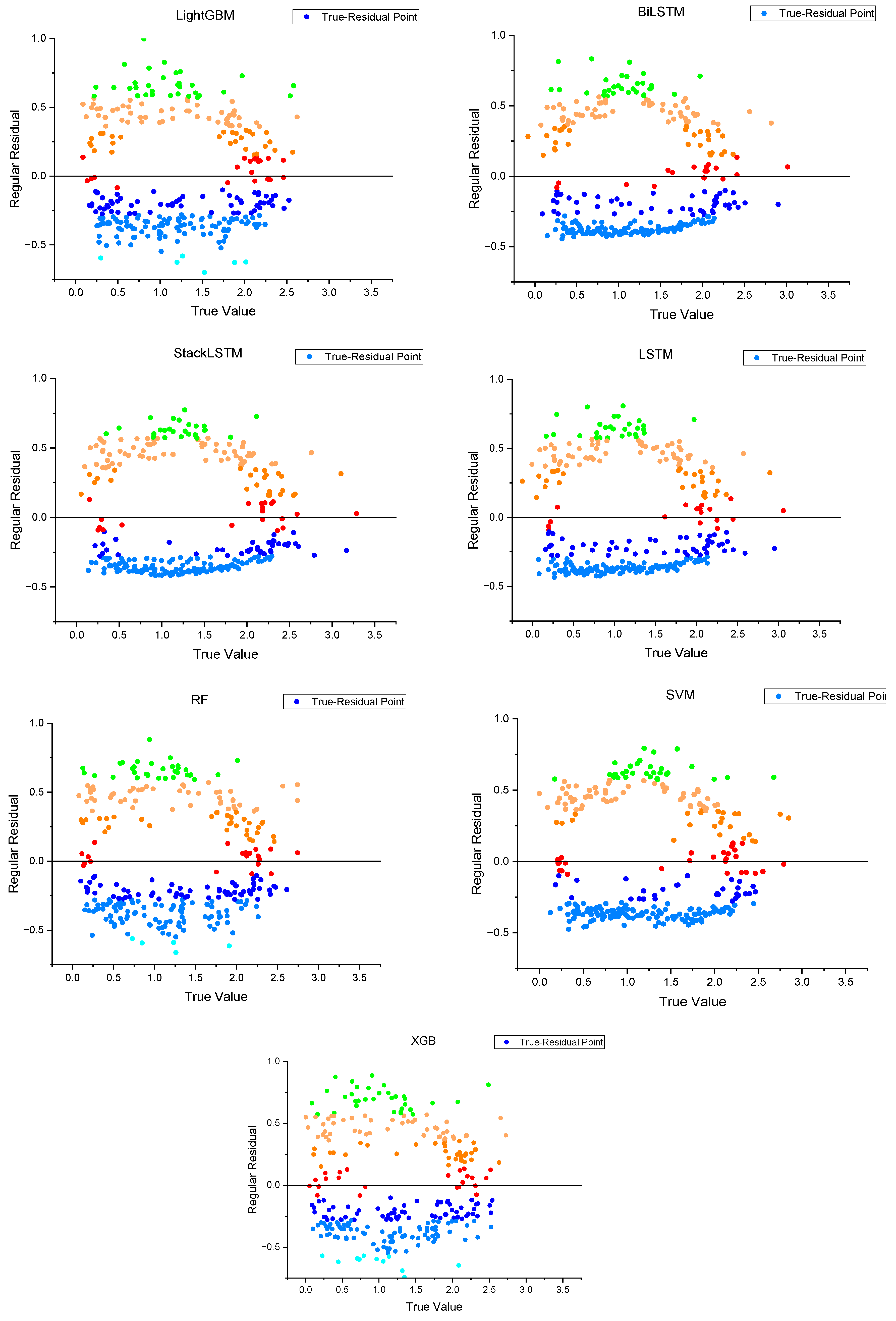
Table 5, Table 6 and Table 7 show that the deep learning-based LSTM, StackLSTM, and BiLSTM models provide the most accurate hourly water level predictions for each measurement station. However, it is worth noting that the results of Table 8 show different prediction results from the other sites, while the results appear in Table 8; the XGB1 model has better prediction results than the LSTM model. To analyze the problem, a residual analysis [49] of the two tables was made to verify the reasons further. Figure A2 shows the residual analysis of the predicted results for the Burlington site using all meteorological factors as the base. From the figure, we can see that the residual dispersion of the deep learning-based LSTM model and its variants is lower, and it can be concluded from Figure A1 that the deep learning-based LSTM model and its variants have more stable performance in water level prediction.

3.3. Seasonal Analysis of Predicted Water Levels

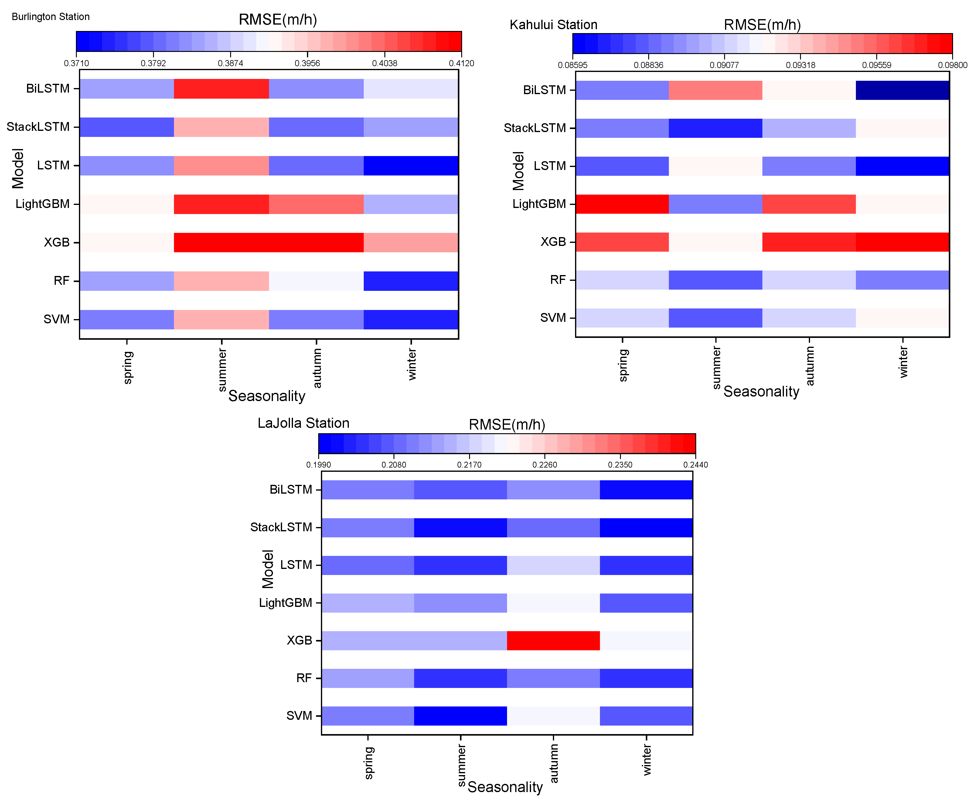
From Figure 7, it can be clearly seen that the water level is cyclical, and analyzing its level according to seasonality is an important task. In previous studies involving meteorology, there are many studies trying to explore the effect of season on the prediction target [50,51]. In this experiment, the water levels of four seasons of the year were verified by predicting the water levels in the months of 3, 6, 9, 12 (spring, summer, fall, and winter) by using the months of January–February, April–May, July–August, and October–November as the training set, respectively. From Figure 8, it is clear that all models have the best prediction results for spring. StackLSTM is more stable in predicting the water level in all seasons, and also the deep learning-based LSTM model and its variants show good prediction results in predicting the water level in all seasons in all sites. The results show that StackLSTM is the most stable in predicting the water level in all seasons.

3.4. Application of CEEMDAN to the Prediction Accuracy of Individual Models Based on All Meteorological Combinations

Based on the condition of not including CEEMDAN, the best input combination was selected as the input for each CEEMDAN model to explore its predictive accuracy under the optimal combination. The results in Table 8 clearly show a significant improvement compared to the results without the CEEMDAN algorithm. Based on the La Jolla site, after incorporating CEEMDAN, the BiLSTM outperformed the original R, RMSE, MAE, and nRMSE, represented by 19.2%, 73.49%, 72.02%, and 72.07%, respectively. This indicates that CEEMDAN demonstrates excellent capabilities in handling non-linear and highly variable data. Table 8 shows that by adding CEEMDAN to the deep learning models LSTM, StackLSTM, and BiLSTM, the predictive results surpass those obtained from four machine learning algorithms: RF, XGB, SVM, and LightGBM. This finding better illustrates the superior predictive performance of deep learning-based LSTM and its variants in time series tasks. Furthermore, BiLSTM demonstrated the best predictive performance at both Burlington and La Jolla sites, yielding a favorable result with RMSE=0.982 m h 1 when predicting water levels at Burlington site, which is 39.2% lower than the lowest RMSE. A slightly different phenomenon was observed at the Kahului site compared to LSTM, but the differences were minor, likely due to the use of identical parameters. However, in the prediction of the Kahului site, the BiLSTM model outperforms the lowest SVM model by 84.39% in terms of RMSE, and the difference in RMSE compared to LSTM is only 0.2%. These findings collectively highlight the superior performance of deep-learning-based LSTM models in predicting time series tasks. From the experimental results, it is also evident that BiLSTM is more suitable for the CEEMDAN algorithm, and the data processed by CEEMDAN can yield better prediction results.
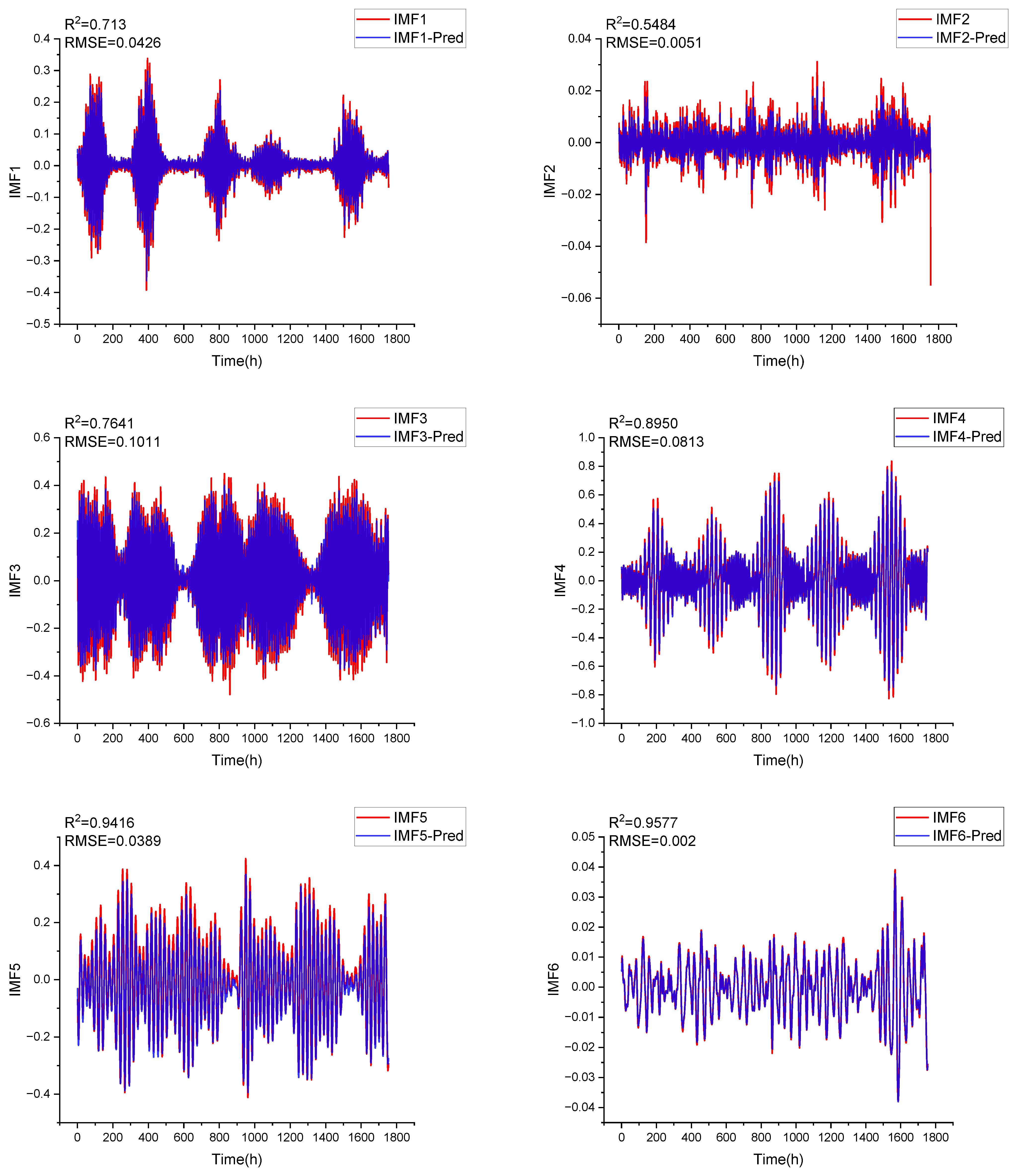
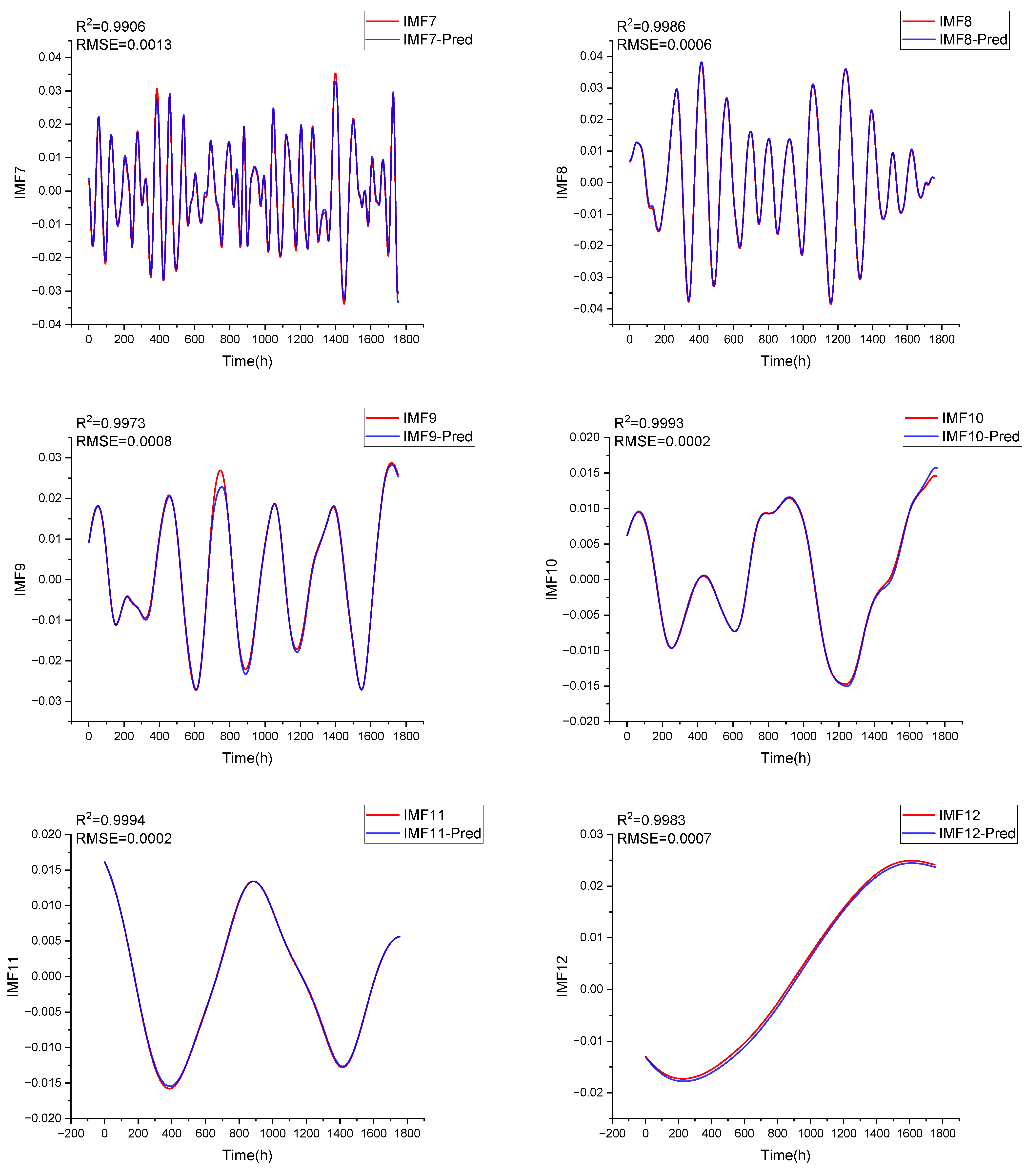
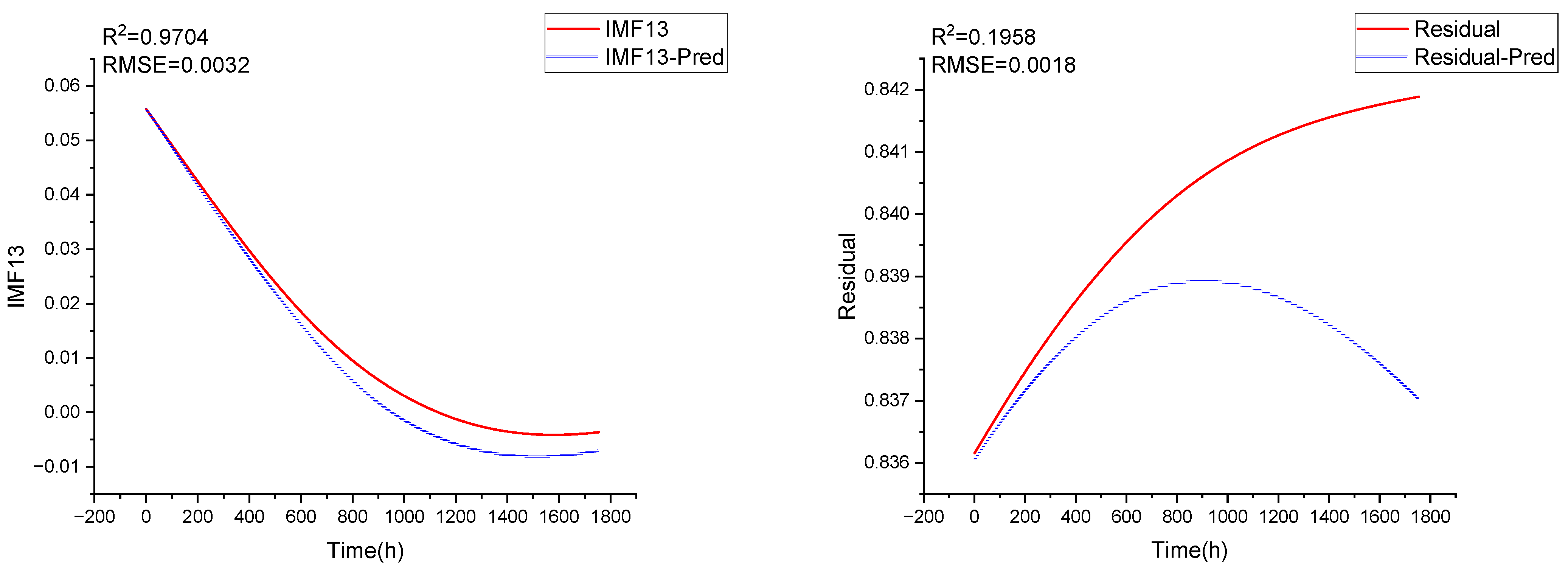
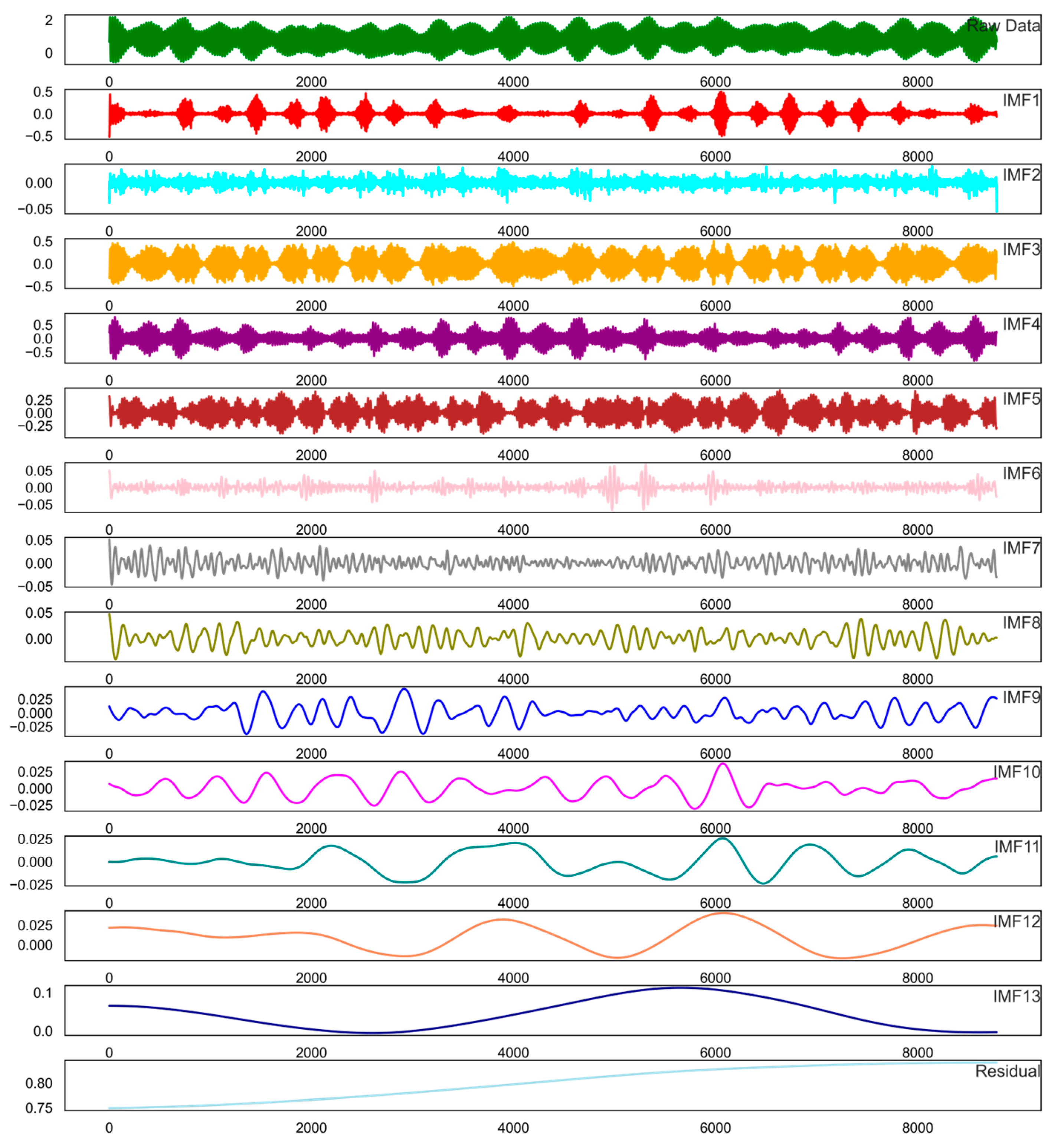
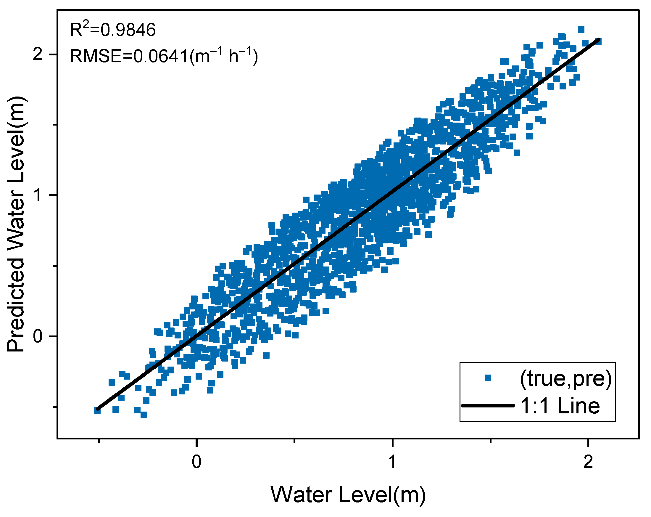
In order to further investigate the principles and performance of applying CEEMDAN to the BiLSTM model for prediction, we conducted a detailed analysis based on the La Jolla site. Figure 9 shows that we decomposed the original signal into 13 intrinsic mode functions (IMFs) and one residual component, which are then separately fed into the model for prediction. Figure A2 shows that BiLSTM exhibits high accuracy in predicting the decomposed signals, with the precision gradually improving as the decomposition iterations increase. This indicates that BiLSTM performs well in predicting the data from each decomposition step of CEEMDAN and adapts better to the patterns present in the decomposed signals. Figure 10 demonstrates the satisfactory results obtained for the final predictions, further highlighting that the deep learning-based BiLSTM model is better suited for adapting to the decomposition signals of CEEMDAN, thus achieving optimal final prediction results.

4. Discussion

Hourly water level variations provide an essential database for better development of tidal power generation, and water level prediction plays an essential role in many fields. Assem et al. used the deep convolutional networks (DeepCNNs) to predict the water level of different sites over a long time [10]. It had higher accuracy than ANNs, support vector machines (SVMs), wavelet transform coupled with an artificial neural networks (WANNs), and wavelet transform coupled with SVMs models. For example, the prediction results of the water level at the Lower Shannon site were that the R 2 of DeepCNNs is 0.87. The R 2 of ANNs is 0.853, the R 2 of SVMs is 0.842, the R 2 of WANNs is 0.854, and the R 2 of WSVMs is 0.842. Similar to the results of this experiment, the prediction results of the deep learning-based StackLSTM model optimize the traditional machine learning models as well as LSTM and BiLSTM in sites at Burlington, Kahului, and La Jolla. This is closely related to the LSTM with multiple layers of LSTMs and the parameter sharing between the multiple layers of LSTMs, which improves the model’s generalization ability. However, StackLSTM fails to reach the global optimum, probably due to the parameter uniformity of its model, which tends to give unsatisfactory results with uniform parameters when the data vary. This depends on the applicability of its model to large-scale as well as high-latitude data. In this experiment, water levels were predicted at three stations. Better predictions were obtained when WS, WD, WG, AT, Baro, and WL were inputs in the Burlington and Kahului stations. Studies similar to this experiment include that of Zhao et al. who used a machine learning model to simulate solar radiation with different combinations of meteorological factors as inputs and concluded that when all meteorological factors were used as inputs, the simulation accuracy was the highest [45]. This indirectly indicates that these meteorological factors are correlated with water levels. The highest predictions were obtained for inputs under the AT, Baro, and WL combination at the La Jolla site. The reason for this phenomenon, as mentioned above, is that StackLSTM did not achieve the global optimal prediction results. After grid search hyperparameter validation, it was found that the parameter-optimized StackLSTM could achieve the best results. The reasons for not doing this will be expanded in the next section of the discussion.
Tidal power generation uses the difference in water levels between high and low tide through a tidal device to accumulate water in a basin and then release it through a turbine [2]. The transformation of the predicted water level allows an improved the optimization of the tidal device, and mastering the hour-by-hour small-scale water level transformation is also adapted to the needs of tidal power generation. This study mainly uses LSTM and its variants as the primary model for predicting water level, and one of the most apparent differences between deep learning and machine learning is the problem of model parameters [52]. The LSTM model contains many parameters, and in this experiment, the LSTM is used as the basis for implementing the algorithm through the Keras Learning package in the TensorFlow framework. The uniform parameters of LSTM in this paper are number of neurons = 200, the activation function is ReLU, dense (full connectivity layer) is 1, the optimizer is Adam, and learning rate is default. The uniform parameters are kept for prediction at all sites to verify the generalizability of this model under uniform parameters, and no adjustment of parameters is made. The results in Table 5, Table 6 and Table 7 of this experiment show that the LSTM and its prediction results are good even with uniform parameters, indirectly showing that the model with uniform parameters can achieve good prediction results. When we use optimization parameters, it accordingly increases the computational time cost [53]. Therefore, it is recommended that when using deep learning models for prediction experiments, when making predictions for different sites or regions, the deep learning models can be validated for higher prediction accuracy than traditional machine learning models by debugging one site and then using it as a parameter for the models in other sites.
In the last part of this paper, CEEMDAN was introduced in an attempt to improve predictive performance under basic conditions. From Table 8, we can clearly see that after introducing CEEMDAN, machine learning algorithms XGB, RF, SVM, and LightGBM, and deep learning algorithms LSTM, StackLSTM, and BiLSTM all showed significant improvements in predictive results compared to the processing of raw signals without CEEMDAN. When CEEMDAN was not used, StackLSTM achieved the best predictive performance. However, after introducing CEEMDAN, BiLSTM actually showed the best predictive results. The experiments demonstrate the compatibility and strong adaptability of LSTM and its variants with other algorithms, leading to better results in predictive tasks. Within the context of CEEMDAN, based on Table 8, it is evident that for any given site, the deep learning models’ predictions outperformed the non-CEEMDAN counterparts. This indicates that LSTM and its variants are better suited for combination with CEEMDAN in predictive tasks. As shown in Figure A2, BiLSTM demonstrated consistently low RMSE values for the IMF modal signals obtained from CEEMDAN, leading to favorable outcomes in each prediction. Additionally, the fitting scatter plot in Figure 10 illustrates the satisfactory water level prediction accuracy of BiLSTM for the La Jolla site. Therefore, it is recommended to utilize deep learning LSTM models and their variants for validation in time series prediction tasks.

5. Conclusions

This paper uses four machine learning algorithms with three algorithms based on deep learning, namely SVM, RF, XGB, LightGBM, LSTM, StackLSTM, and BiLSTM models, based on hour-by-hour meteorological data and water levels from the Burlington, Kahului and La Jolla sites. The meteorological data and water levels at three stations from 1 January 2022 to 1 January 2023 were divided into four combinations as the input of each model to investigate the effect of meteorological factors on predicting the hour-by-hour water level prediction accuracy at these three stations. The results showed that the highest prediction accuracy was achieved at the Burlington and Kahului sites when all the meteorological factors WS, WD, WG, AT, Baro, and WL were used as inputs, which indicates the importance of meteorological factors for water level prediction. In comparing deep learning and machine learning, the StackLSTM model based on the deep learning algorithm achieved the best prediction results in most cases. However, the problem of the LSTM model and its variants of the model under the same parameters results in not obtaining globally optimal predictions. The results showed that the LSTM model did not achieve the highest accuracy in its predictions for the La Jolla site with uniform parameters. Meanwhile, in the analysis of the predictions for the four seasons, the results show that StackLSTM performs the most consistently and that the deep-learning-based LSTM model and its variants also outperform the traditional machine learning model. In the final part of this paper, the CEEMDAN algorithm was introduced into various models, and the optimal input combinations without CEEMDAN were used as the input strategy after incorporating CEEMDAN. The results showed a significant improvement in predictive accuracy after incorporating CEEMDAN. The deep learning model BiLSTM achieved the best predictive results at each site. Additionally, experimental findings revealed that even with the inclusion of CEEMDAN, the deep learning LSTM model and its variants still outperformed the various machine learning models proposed in this paper. This indicates that in time series prediction tasks, deep learning LSTM and its variants are more compatible with CEEMDAN and can achieve better predictive results.
This study investigates the effect of meteorological factors on predicted water levels to provide a reference for water level prediction for the development of tidal power generation. However, water level prediction at different time scales has different applications, and more work is needed to evaluate the performance of these models on a day-by-day scale. Further research is required for multi-step forecasting as well. Predicting by 3, 5, and 7 h at once is an important task that remains to be completed. Secondly, the time cost of each model is not calculated in this experiment. In future work, we should try to use different algorithms and optimization algorithms to comprehensively analyze which models have more application value, such as convolutional neural network-long short-term memory (CNN-LSTM), attention long short-term memory (Attention-LSTM), or add a grid search algorithm, particle swarm optimization (PSO), and other optimization algorithms based on the above-mentioned, which need to be further studied.

Author Contributions

Conceptualization, Z.Y. and L.W.; methodology, Z.Y. and L.W.; software, Z.Y.; validation, Z.Y., L.W. and X.L.; formal analysis, Z.Y. and L.W.; investigation, Z.Y., L.W. and X.L.; resources, Z.Y. and L.W.; data curation, Z.Y.; writing—original draft preparation, Z.Y.; writing—review and editing, Z.Y. and L.W.; visualization, Z.Y. and L.W.; supervision, Z.Y., L.W. and X.L.; project administration, X.L.; funding acquisition, X.L. All authors have read and agreed to the published version of the manuscript.

Funding

This research was funded by the Natural Science Foundation Project of Jiangxi Province, grant number 20232BAB205031, the National Natural Science Foundation of China, grant number 52269013, Jiangxi Provincial Science and Technology Department Major Science and Technology Project of China, grant number 20203ABC28W016-01-04, Jiangxi Forestry Bureau camphor tree research project of China, grant number 202007-01-04.

Data Availability Statement

We utilized an open-source dataset from the National Oceanic and Atmospheric Administration (NOAA) of the United States: https://tidesandcurrents.noaa.gov (accessed on 5 September 2023).

Acknowledgments

We would like to express our special thanks to the National Oceanic and Atmospheric Administration (NOAA) of the United States for providing the foundational data for this research.

Conflicts of Interest

The authors declare no conflict of interest.

Appendix A

Figure A1. Residual scatter plots of predicted water levels at the Burlington site under seven models with all meteorological factors as inputs.
Water 15 03190 g0a1
Figure A2. The prediction results for each IMF mode and residual obtained from the CEEMDAN decomposition of water level data at site Burlington.
Water 15 03190 g0a2aWater 15 03190 g0a2bWater 15 03190 g0a2c

Appendix B

The code for this study is available at: https://github.com/AnleHrc/CEEMDAN_LSTM_ML_Prediction_NOAA_WaterLevel (accessed on 5 September 2023).

References

  1. Wang, Z.; Wang, Z. A review on tidal power utilization and operation optimization. In IOP Conference Series: Earth and Environmental Science; IOP Publishing: Bristol, UK, 2019; p. 052015. [Google Scholar]
  2. Roberts, A.; Thomas, B.; Sewell, P.; Khan, Z.; Balmain, S.; Gillman, J. Current tidal power technologies and their suitability for applications in coastal and marine areas. J. Ocean. Eng. Mar. Energy 2016, 2, 227–245. [Google Scholar] [CrossRef]
  3. Khan, M.S.; Coulibaly, P. Application of Support Vector Machine in Lake Water Level Prediction. J. Hydrol. Eng. 2006, 11, 199–205. [Google Scholar] [CrossRef]
  4. Shiri, J.; Shamshirband, S.; Kisi, O.; Karimi, S.; Bateni, S.M.; Hosseini Nezhad, S.H.; Hashemi, A. Prediction of Water-Level in the Urmia Lake Using the Extreme Learning Machine Approach. Water Resour. Manag. 2016, 30, 5217–5229. [Google Scholar] [CrossRef]
  5. Azad, A.S.; Sokkalingam, R.; Daud, H.; Adhikary, S.K.; Khurshid, H.; Mazlan, S.N.A.; Rabbani, M.B.A. Water level prediction through hybrid SARIMA and ANN models based on time series analysis: Red hills reservoir case study. Sustainability 2022, 14, 1843. [Google Scholar] [CrossRef]
  6. Panyadee, P.; Champrasert, P.; Aryupong, C. Water level prediction using artificial neural network with particle swarm optimization model. In Proceedings of the 2017 5th International Conference on Information and Communication Technology (ICoIC7), Melaka, Malaysia, 17–19 May 2017; pp. 1–6. [Google Scholar]
  7. Wang, B.; Wang, B.; Wu, W.; Xi, C.; Wang, J. Sea-water-level prediction via combined wavelet decomposition, neuro-fuzzy and neural networks using SLA and wind information. Acta Oceanol. Sin. 2020, 39, 157–167. [Google Scholar] [CrossRef]
  8. LeCun, Y.; Bengio, Y.; Hinton, G. Deep learning. Nature 2015, 521, 436–444. [Google Scholar] [CrossRef]
  9. Noor, F.; Haq, S.; Rakib, M.; Ahmed, T.; Jamal, Z.; Siam, Z.S.; Hasan, R.T.; Adnan, M.S.G.; Dewan, A.; Rahman, R.M. Water level forecasting using spatiotemporal attention-based long short-term memory network. Water 2022, 14, 612. [Google Scholar] [CrossRef]
  10. Assem, H.; Ghariba, S.; Makrai, G.; Johnston, P.; Gill, L.; Pilla, F. Urban water flow and water level prediction based on deep learning. In Machine Learning and Knowledge Discovery in Databases: European Conference, ECML PKDD 2017, Skopje, Macedonia, 18–22 September 2017, Proceedings, Part III 10, 2017; Springer International Publishing: Cham, Switzerland, 2017; pp. 317–329. [Google Scholar]
  11. Zhang, Z.; Qin, H.; Yao, L.; Liu, Y.; Jiang, Z.; Feng, Z.; Ouyang, S.; Pei, S.; Zhou, J. Downstream water level prediction of reservoir based on convolutional neural network and long short-term memory network. J. Water Resour. Plan. Manag. 2021, 147, 04021060. [Google Scholar] [CrossRef]
  12. Hopfield, J.J. Neural networks and physical systems with emergent collective computational abilities. Proc. Natl. Acad. Sci. USA 1982, 79, 2554–2558. [Google Scholar] [CrossRef]
  13. Chung, J.; Gulcehre, C.; Cho, K.; Bengio, Y. Empirical Evaluation of Gated Recurrent Neural Networks on Sequence Modeling. arXiv 2014, arXiv:1412.3555. [Google Scholar]
  14. Hochreiter, S.; Schmidhuber, J. Long Short-Term Memory. Neural Comput. 1997, 9, 1735–1780. [Google Scholar] [CrossRef]
  15. Pan, M.; Zhou, H.; Cao, J.; Liu, Y.; Hao, J.; Li, S.; Chen, C.-H. Water level prediction model based on GRU and CNN. IEEE Access 2020, 8, 60090–60100. [Google Scholar] [CrossRef]
  16. Baek, S.-S.; Pyo, J.; Chun, J.A. Prediction of Water Level and Water Quality Using a CNN-LSTM Combined Deep Learning Approach. Water 2020, 12, 3399. [Google Scholar] [CrossRef]
  17. Zan, Y.; Gao, Y.; Jiang, Y.; Pan, Y.; Li, X.; Su, P. The Effects of Lake Level and Area Changes of Poyang Lake on the Local Weather. Atmosphere 2022, 13, 1490. [Google Scholar] [CrossRef]
  18. Behzad, M.; Asghari, K.; Coppola, E.A., Jr. Comparative study of SVMs and ANNs in aquifer water level prediction. J. Comput. Civ. Eng. 2010, 24, 408–413. [Google Scholar] [CrossRef]
  19. Choi, C.; Kim, J.; Han, H.; Han, D.; Kim, H.S. Development of water level prediction models using machine learning in wetlands: A case study of Upo wetland in South Korea. Water 2019, 12, 93. [Google Scholar] [CrossRef]
  20. Arkian, F.; Nicholson, S.E.; Ziaie, B. Meteorological factors affecting the sudden decline in Lake Urmia’s water level. Theor. Appl. Climatol. 2018, 131, 641–651. [Google Scholar] [CrossRef]
  21. Cox, D.T.; Tissot, P.; Michaud, P. Water Level Observations and Short-Term Predictions Including Meteorological Events for Entrance of Galveston Bay, Texas. J. Waterw. Port Coast. Ocean. Eng. 2002, 128, 21–29. [Google Scholar] [CrossRef]
  22. Yadav, B.; Eliza, K. A hybrid wavelet-support vector machine model for prediction of Lake water level fluctuations using hydro-meteorological data. Measurement 2017, 103, 294–301. [Google Scholar] [CrossRef]
  23. Lu, H.; Ma, X. Hybrid decision tree-based machine learning models for short-term water quality prediction. Chemosphere 2020, 249, 126169. [Google Scholar] [CrossRef]
  24. Gutman, G.; Ignatov, A. The derivation of the green vegetation fraction from NOAA/AVHRR data for use in numerical weather prediction models. Int. J. Remote Sens. 1998, 19, 1533–1543. [Google Scholar] [CrossRef]
  25. Gruber, A.; Krueger, A.F. The Status of the NOAA Outgoing Longwave Radiation Data Set. Bull. Am. Meteorol. Soc. 1984, 65, 958–962. [Google Scholar] [CrossRef]
  26. Cortes, C.; Vapnik, V. Support-vector networks. Mach. Learn. 1995, 20, 273–297. [Google Scholar] [CrossRef]
  27. Noble, W.S. What is a support vector machine? Nat. Biotechnol. 2006, 24, 1565–1567. [Google Scholar] [CrossRef]
  28. Pai, P.-F.; Lin, C.-S. A hybrid ARIMA and support vector machines model in stock price forecasting. Omega 2005, 33, 497–505. [Google Scholar] [CrossRef]
  29. Suykens, J.A.; Vandewalle, J. Least squares support vector machine classifiers. Neural Process. Lett. 1999, 9, 293–300. [Google Scholar] [CrossRef]
  30. Breiman, L. Random forests. Mach. Learn. 2001, 45, 5–32. [Google Scholar] [CrossRef]
  31. Qi, Y. Random forest for bioinformatics. In Ensemble Machine Learning: Methods and Applications; Springer: New York, NY, USA, 2012; pp. 307–323. [Google Scholar]
  32. Janitza, S.; Tutz, G.; Boulesteix, A.-L. Random forest for ordinal responses: Prediction and variable selection. Comput. Stat. Data Anal. 2016, 96, 57–73. [Google Scholar] [CrossRef]
  33. Chen, T.; Guestrin, C. Xgboost: A scalable tree boosting system. In Proceedings of the 22nd ACM SIGKDD International Conference on Knowledge Discovery and Data Mining, San Francisco, CA, USA, 13–17 August 2016; pp. 785–794. [Google Scholar]
  34. Wang, C.; Deng, C.; Wang, S. Imbalance-XGBoost: Leveraging weighted and focal losses for binary label-imbalanced classification with XGBoost. Pattern Recognit. Lett. 2020, 136, 190–197. [Google Scholar] [CrossRef]
  35. Ke, G.; Meng, Q.; Finley, T.; Wang, T.; Chen, W.; Ma, W.; Ye, Q.; Liu, T.-Y. Lightgbm: A highly efficient gradient boosting decision tree. In Advances in Neural Information Processing Systems; Curran Associates Inc.: Red Hook, NY, USA, 2017; Volume 30. [Google Scholar]
  36. Chen, C.; Zhang, Q.; Ma, Q.; Yu, B. LightGBM-PPI: Predicting protein-protein interactions through LightGBM with multi-information fusion. Chemom. Intell. Lab. Syst. 2019, 191, 54–64. [Google Scholar] [CrossRef]
  37. Janiesch, C.; Zschech, P.; Heinrich, K. Machine learning and deep learning. Electron. Mark. 2021, 31, 685–695. [Google Scholar] [CrossRef]
  38. Gers, F.A.; Schmidhuber, J.; Cummins, F. Learning to forget: Continual prediction with LSTM. Neural Comput. 2000, 12, 2451–2471. [Google Scholar] [CrossRef] [PubMed]
  39. Zhang, W.; Bai, K.; Zhan, C.; Tu, B. Parameter prediction of coiled tubing drilling based on GAN–LSTM. Sci. Rep. 2023, 13, 10875. [Google Scholar] [CrossRef] [PubMed]
  40. Dyer, C.; Ballesteros, M.; Ling, W.; Matthews, A.; Smith, N.A. Transition-based dependency parsing with stack long short-term memory. arXiv 2015, arXiv:1505.08075. [Google Scholar]
  41. Pattana-Anake, V.; Joseph, F.J.J. Hyper parameter optimization of stack LSTM based regression for PM 2.5 data in Bangkok. In Proceedings of the 2022 7th International Conference on Business and Industrial Research (ICBIR), Bangkok, Thailan, 19–20 May 2022; pp. 13–17. [Google Scholar]
  42. Schuster, M.; Paliwal, K.K. Bidirectional recurrent neural networks. IEEE Trans. Signal Process. 1997, 45, 2673–2681. [Google Scholar] [CrossRef]
  43. Ma, X.; Hovy, E. End-to-end sequence labeling via bi-directional lstm-cnns-crf. arXiv 2016, arXiv:1603.01354. [Google Scholar]
  44. Joseph, R.V.; Mohanty, A.; Tyagi, S.; Mishra, S.; Satapathy, S.K.; Mohanty, S.N. A hybrid deep learning framework with CNN and Bi-directional LSTM for store item demand forecasting. Comput. Electr. Eng. 2022, 103, 108358. [Google Scholar] [CrossRef]
  45. Cui, Y.; Jia, L.; Fan, W. Estimation of actual evapotranspiration and its components in an irrigated area by integrating the Shuttleworth-Wallace and surface temperature-vegetation index schemes using the particle swarm optimization algorithm. Agric. For. Meteorol. 2021, 307, 108488. [Google Scholar] [CrossRef]
  46. Fan, J.; Yue, W.; Wu, L.; Zhang, F.; Cai, H.; Wang, X.; Lu, X.; Xiang, Y. Evaluation of SVM, ELM and four tree-based ensemble models for predicting daily reference evapotranspiration using limited meteorological data in different climates of China. Agric. For. Meteorol. 2018, 263, 225–241. [Google Scholar] [CrossRef]
  47. Chang, K.-M. Ensemble empirical mode decomposition for high frequency ECG noise reduction. Biomed. Technol. 2010, 55, 193–201. [Google Scholar] [CrossRef]
  48. Torres, M.E.; Colominas, M.A.; Schlotthauer, G.; Flandrin, P. A complete ensemble empirical mode decomposition with adaptive noise. In Proceedings of the 2011 IEEE International Conference on Acoustics, Speech and Signal Processing (ICASSP), Prague, Czech Republic, 22–27 May 2011; pp. 4144–4147. [Google Scholar]
  49. Fernandez, G.C. Residual analysis and data transformations: Important tools in statistical analysis. HortScience 1992, 27, 297–300. [Google Scholar] [CrossRef]
  50. Atashi, V.; Gorji, H.T.; Shahabi, S.M.; Kardan, R.; Lim, Y.H. Water level forecasting using deep learning time-series analysis: A case study of red river of the north. Water 2022, 14, 1971. [Google Scholar] [CrossRef]
  51. Hsu, K.l.; Gupta, H.V.; Sorooshian, S. Artificial neural network modeling of the rainfall-runoff process. Water Resour. Res. 1995, 31, 2517–2530. [Google Scholar] [CrossRef]
  52. Xin, Y.; Kong, L.; Liu, Z.; Chen, Y.; Li, Y.; Zhu, H.; Gao, M.; Hou, H.; Wang, C. Machine learning and deep learning methods for cybersecurity. IEEE Access 2018, 6, 35365–35381. [Google Scholar] [CrossRef]
  53. Li, L.; Jamieson, K.; Rostamizadeh, A.; Gonina, E.; Hardt, M.; Recht, B.; Talwalkar, A. Massively parallel hyperparameter tuning. arXiv 2018, arXiv:1810.05934. [Google Scholar]
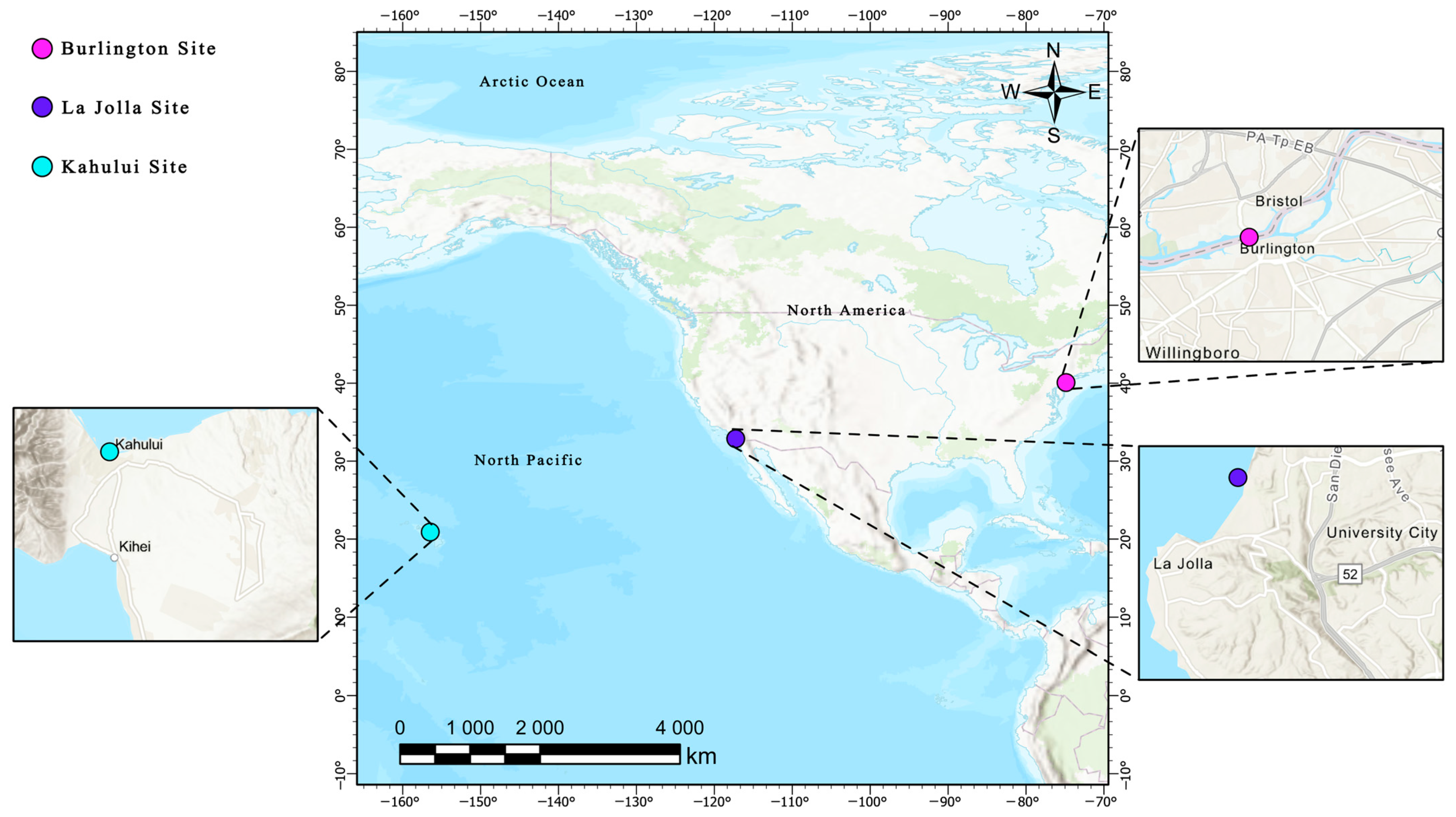
Figure 1. The three water level monitoring stations studied in this paper.
Water 15 03190 g001
Figure 2. Violin analysis plots of meteorological (WS, WG, AT)—water level data for two stations, (a,b): Kahului and La Jolla stations, respectively.
Water 15 03190 g002
Figure 3. LSTM basic cell structure.
Water 15 03190 g003
Figure 4. Two-layer stackLSTM basic cell structure.
Water 15 03190 g004
Figure 5. BiLSTM basic cell structure.
Water 15 03190 g005
Figure 6. CEEMDAN-LSTM forecasting process; note that the LSTM part of it can be replaced with other models for the prediction task.
Water 15 03190 g006
Figure 7. Prediction curves of each model for three stations when all meteorological factors are used as inputs. The right histogram’s L-G, B-L, S-L, and L represent LightGBM, BiLSTM, StackLSTM, and LSTM, respectively.
Water 15 03190 g007aWater 15 03190 g007b
Figure 8. RMSE thermal analysis of each model’s prediction results for all seasons under all combinations of meteorological factors.
Water 15 03190 g008
Figure 9. CEEMDAN signal decomposition of water level data at the La Jolla site.
Water 15 03190 g009
Figure 10. CEEMDAN-BiLSTM predictions of water level at the La Jolla site based on input combinations of all meteorological factors.
Water 15 03190 g010
Table 1. Detailed statistics from the Burlington site.
Burlington
VariableWind Speed
(m/s)
Wind Dir
(deg)
Wind Gust
(m/s)
Air Temp
(°C)
Baro
(mb)
Water Level
(m)
Mean 2.674197.1734.21213.2791017.3971.316
Std 1.954103.0322.89510.1747.6193760.793
Min 0.0000.0000.000−13.400985.000−0.595
Q 1 1.20093.0001.9005.30001012.7000.621
Q 2 2.300229.0003.70013.6001016.9001.307
Q 3 3.800283.0005.80021.8001022.3002.028
Max 13.100360.00021.30035.0001040.6003.278
Note: Std represents the standard deviation, and Q1–Q3 represents 25%, 50%, and 75% of the total data. For more visual analysis of visualization, the data analysis graphs of the remaining two sites are displayed using violin plots.
Table 2. Detailed WG and BARO statistics from the Kahului and La Jolla sites.
SiteKahuluiLa Jolla
VariableWind Dir
(deg)
Baro
(mb)
Wind Dir
(deg)
Baro
(mb)
Mean 94.6081016.683198.0911015.177
Std 90.1152.348102.6643.867
Min 0.000997.7000.000998.600
Q 1 45.0001015.400114.0001012.500
Q 2 66.0001016.800213.5001014.700
Q 3 82.0001018.200286.0001017.700
Max 360.0001023.100360.0001027.600
Note: Std represents the standard deviation, and Q1–Q3 represents 25%, 50%, and 75% of the total data. For more visual analysis of visualization, the data analysis graphs of the remaining two sites are displayed using violin plots.
Table 3. Combination of meteorological water level variable inputs for different machine learning models and deep learning models.
Input CombinationsSVMRFXGBLightGBMLSTMStackLSTMBiLSTM
WS, WD, WG, AT, Baro, WLSVM1RF1XGB1LightGBM1LSTM1StackLSTM1BiLSTM1
WS, WD, WG, WLSVM2RF2XGB2LightGBM2LSTM2StackLSTM2BiLSTM2
AT, Baro, WLSVM3RF3XGB3LightGBM3LSTM3StackLSTM3BiLSTM3
WL, WS, ATSVM4RF4XGB4LightGBM4LSTM4StackLSTM4BiLSTM4
Table 4. Parameter settings for each model.
SiteModelsParameters
Burlington, Kahului, La JollaSVMKernel: RBF
RFN_Estimators: 50, Oob_Score: True, N_Jobs: −1, Random_State: 50, Max_Features: 1.0, Min_Samples_leaf: 10
XGBObjective: reg:squarederror, N_Estimatorsl: 50
LightGBMBoosting Type: Gbdt, Objective: Regression, Num_Leaves: 29, Learning_Rate: 0.09, Feature_Fraction: 0.9, Bagging_Fraction: 0.8, Bagging_Freq: 6
LSTMLayers: 1, Number of Neurons: 200, Dense: 1, Activation: ReLU, Optimizer: Adam, Loss Function: MSE, Epochs: 40, Batch Size: 1
StackLSTMLayers: 2, Number of Neurons: 200 (2×100), Dense: 1, Activation: ReLU, Optimizer: Adam, Loss Function: MSE, Epochs: 40, Batch Size: 1
BiLSTMLayers: 2, Number of Neurons: 200 (2×100), Dense: 1, Activation: ReLU, Optimizer: Adam, Loss Function: MSE, Epochs: 40, Batch Size: 1
Table 5. Predictions of seven models at Burlington station under different input combinations.
ModelStatistical IndicatorsModelStatistical Indicators
Input R 2 MAE
mh−1
RMSE
mh−1
nRMSE R 2 MAE
mh−1
RMSE
mh−1
nRMSE
WS, WD, WG, AT, Baro, WL WS, WD, WG, WL
SVM10.6880.3580.3890.111SVM20.6960.3610.3870.110
RF10.6920.3570.3980.110RF20.6860.3560.3950.112
XGB10.6800.3590.4120.110XGB20.6580.3630.4090.116
LightGBM10.6890.3470.3930.110LightGBM20.6820.3510.3900.110
LSTM10.6950.3460.3920.112LSTM20.6860.3500.3870.110
StackLSTM10.7210.3670.3910.110StackLSTM20.7190.3560.3840.109
BiLSTM10.6810.3500.3900.116BiLSTM20.6990.3570.3860.109
WS, AT, WL AT, Baro, WL
SVM30.6820.3640.3910.111SVM40.6980.3620.3900.110
RF30.6890.3620.4010.113RF40.6780.3680.4090.116
XGB30.6740.3660.4190.119XGB40.6620.3710.4280.121
LightGBM30.6980.3530.3990.113LightGBM40.6910.3600.4020.114
LSTM30.6980.3530.3880.110LSTM40.7040.3570.3860.109
StackLSTM30.6950.3460.3920.111StackLSTM40.6890.3470.3910.110
BiLSTM30.7020.3530.3890.110BiLSTM40.7040.3580.3850.109
Note: The best statistical analysis results for machine learning are marked in bold, while the best statistical analysis results for the LSTM model and its variants are highlighted in orange.
Table 6. Predictions of seven models at Kahului station under different input combinations.
ModelStatistical IndicatorsModelStatistical Indicators
Input R 2 MAE
mh−1
RMSE
mh−1
nRMSE R 2 MAE
mh−1
RMSE
mh−1
nRMSE
WS, WD, WG, AT, Baro, WL WS, WD, WG, WL
SVM10.8430.0730.0900.077SVM20.8380.0750.0930.079
RF10.8370.0740.0950.081RF20.8310.0760.0960.082
XGB10.8360.0760.0950.081XGB20.8150.0800.1000.085
LightGBM10.8450.0740.0920.078LightGBM20.8400.0750.0930.079
LSTM10.8380.0740.0930.080LSTM20.8350.0740.0940.080
StackLSTM10.8520.0730.0920.078StackLSTM20.8470.0740.0930.079
BiLSTM10.8380.0730.0930.079BiLSTM20.8420.0740.0940.080
WS, AT, WL AT, Baro, WL
SVM30.8390.0740.0930.079SVM40.8310.0760.0950.081
RF30.8340.0750.0960.082RF40.8390.0750.0950.081
XGB30.8300.0770.0980.083XGB40.8310.0780.0970.083
LightGBM30.8400.0740.0940.080LightGBM40.8320.0760.0960.082
LSTM30.8500.0720.0910.077LSTM40.8360.0740.0940.08
StackLSTM30.8310.0740.0950.081StackLSTM40.8380.0740.0940.08
BiLSTM30.8390.0730.0930.080BiLSTM40.8370.0750.0950.081
Note: The best statistical analysis results for machine learning are marked in bold, while the best statistical analysis results for the LSTM model and its variants are highlighted in orange.
Table 7. Predictions of seven models at La Jolla station under different input combinations.
ModelStatistical IndicatorsModelStatistical Indicators
Input R 2 MAE
mh−1
RMSE
mh−1
nRMSE R 2 MAE
mh−1
RMSE
mh−1
nRMSE
WS, WD, WG, AT, Baro, WL WS, WD, WG, WL
SVM10.8020.1970.2350.086SVM20.8050.1920.2320.085
RF10.8280.1910.2290.084RF20.8180.1940.2340.086
XGB10.8310.1900.2260.083XGB20.8100.1970.2390.088
LightGBM10.8300.1890.2250.082LightGBM20.8210.1930.2320.085
LSTM10.8200.1890.2270.083LSTM20.8170.1930.2330.085
StackLSTM10.8150.1910.2300.084StackLSTM20.8150.1900.2310.085
BiLSTM10.8260.1890.2290.084BiLSTM20.8080.1930.2350.086
WS, AT, WL AT, Baro, WL
SVM30.8200.1910.2290.084SVM40.8130.1930.2300.084
RF30.8260.1930.2310.085RF40.8210.1940.2320.085
XGB30.8310.1910.2320.085XGB40.8330.1890.2280.083
LightGBM30.8330.1910.2280.084LightGBM40.8370.1880.2230.082
LSTM30.8240.1910.2290.084LSTM40.8280.1880.2270.083
StackLSTM30.8300.1910.2280.084StackLSTM40.8270.1890.2260.083
BiLSTM30.8300.1900.2270.083BiLSTM40.8350.1880.2250.082
Note: The best statistical analysis results for machine learning are marked in bold, while the best statistical analysis results for the LSTM model and its variants are highlighted in orange.
Table 8. Water level prediction results for three sites, Burlington, Kahului, and La Jolla, based on the optimal combination of the CEEMDAN algorithm introduced with the input meteorological factors as inputs.
SiteModelStatistical Indicators
Input R 2 MAE
mh−1
RMSE
mh−1
n R M S E
WS, WD, WG, AT, Baro, WL
BurlingtonCEEMDAN-SVM0.96520.11310.14480.0397
CEEMDAN-RF0.97420.10150.12450.0342
CEEMDAN-XGB0.97380.09960.12550.0344
CEEMDAN-LightGBM0.97550.09820.12130.0333
CEEMDAN-LSTM0.98030.08640.10880.0299
CEEMDAN-StackLSTM0.98030.08810.10890.0299
CEEMDAN-BiLSTM0.98200.07900.10400.0285
KahuluiCEEMDAN-SVM0.93170.04750.05960.0474
CEEMDAN-RF0.96950.03170.03990.0317
CEEMDAN-XGB0.96670.03300.04160.0331
CEEMDAN-LightGBM0.96760.03250.04100.0326
CEEMDAN-LSTM0.98000.02540.03220.0256
CEEMDAN-StackLSTM0.97940.02580.03270.0260
CEEMDAN-BiLSTM0.97990.02540.03230.0257
La JollaCEEMDAN-SVM0.94930.08510.11640.0426
CEEMDAN-RF0.97540.06300.08110.0297
CEEMDAN-XGB0.96940.06830.09040.0331
CEEMDAN-LightGBM0.97420.06350.08310.0304
CEEMDAN-LSTM0.98330.05140.06690.0245
CEEMDAN-StackLSTM0.98440.05030.06460.0237
CEEMDAN-BiLSTM0.98460.05010.06410.0235
Note: The best statistical analysis results for machine learning are marked in bold, while the best statistical analysis results for the LSTM model and its variants are highlighted in orange.
Disclaimer/Publisher’s Note: The statements, opinions and data contained in all publications are solely those of the individual author(s) and contributor(s) and not of MDPI and/or the editor(s). MDPI and/or the editor(s) disclaim responsibility for any injury to people or property resulting from any ideas, methods, instructions or products referred to in the content.