
A Review of Data Quality and Cost Considerations for Water Quality Monitoring at the Field Scale and in Small Watersheds

 ,
,
Abstract
:1. Introduction
2. Materials and Methods
3. Results and Discussion
3.1. Monitoring Site Selection and Establishment
3.2. Discharge Data Collection

| Decision | Annual Cost | Initial (One-Time) Cost | Data Uncertainty | Related Comments |
|---|---|---|---|---|
| Number of sites | $$$: technical staff salary | $$$: vehicle | - | Carefully determine the number of sampling sites. One full-time technician can typically operate 6–10 sites (including laboratory analysis, data management), but the distance to and proximity of the sites can affect this. For graduate students, the salary costs are less but so is their capacity in terms of time and expertise. Exceeding a reasonable number of sampling sites and utilizing inexperienced technicians will decrease data quality. |
| Location of sites | $-$$: travel costs = f (location, proximity); site maintenance; equipment maintenance | $/site: basic installation -or- $$/site: extensive berm construction required | - | Locate sites to minimize travel costs. If possible, install field-scale sites within a natural drainage way to avoid extensive berm construction (USDA, 1996), and avoid unstable sites. Commit to frequent maintenance [2,3,7], as less frequent maintenance will decrease data quality due to missing or inaccurate data. |
| Equipment shelter | - | $/site: homemade or repurposed shelter -or- $-$$/site: commercial shelter | - | Install equipment shelter at each site. Ensure accessibility during wet weather, above the flood level [3,25], yet as close as possible to the sample point [32]. |
| Duplicate equipment | - | $$/per every 6–10 sites, backup and replacement equipment | - | Purchase backup and replacement equipment to reduce missing data (increases the data quality). |
| Power needs | $/site: electrical costs (if AC power; maintain and recharge batteries) | $-$$/site: install AC power at remote site (if feasible) -and- $-$$/site: solar panel and battery | See [20,33,34] for uncertainty related to preservation and storage. | Consider power needs based on the QA/QC requirements for sample preservation. Refrigerated samplers often require AC power; however, battery backup is recommended for all automated samplers to avoid power loss during storm events. |
| Communication devices (cell, radio, satellite) | $/site: fees | $-$$/site: communication device | - | Consider the costs and benefits of communication devices (i.e., purchase costs and fees relative to salary and travel costs). The communication device can increase data quality through the immediate notification of equipment failure. As the distance to the sampling sites increases, the benefits of communication devices increases. |
| Decision | Annual Cost | Initial (One-Time) Cost | Data Uncertainty | Related Comments |
|---|---|---|---|---|
| Are discharge (flow) data needed to meet the project objectives? | Cost estimates below apply only to projects that measure loads (project types 3–5 in Table 1). | - | If load data are not needed, discharge measurement is unnecessary; however, flow and load data are often critical, so carefully consider the potential future data uses and project objectives. If flow data are needed, consider the following options. | |
| Discharge (flow) measurement options: | ||||
| Measure the stage in the pre-calibrated flow control structure with the established stage–discharge relationship [7,35] | $/site: maintenance | $$/site: control structure and stage measurement equipment | ±5–10% depending on frequency of calibration with a current meter [36] | Follow installation and maintenance recommendations [32,37]. Data quality decreases substantially if the stage exceeds the design capability, which limits use as the contributing area increases. |
| Measure the stage in a channel, culvert, or other stable flow path | $-$$/site: maintenance; flow measurements and cross-section surveys to confirm or adjust the stage–discharge relationship | $-$$/site: survey cross- section; stage measurement equipment | Stable channel: ±6% [38], ±10% [36] Shifting channel: ±20% [36] | Selecting sites with an established stage–discharge relationship and in a stable channel avoids the cost and difficulty of developing and adjusting the relationship. Calibrate the stage–discharge relationship with a current meter and cross-section surveys, 8–12 per year especially in shifting channels. |
| Measure discharge with area–velocity sensor | $-$$/site: maintenance; flow measurements and channel surveys to confirm discharge data | $$/site: survey cross- section; velocity measurement equipment | >10% (King, unpublished data) ±10% in trapezoidal channel [39] ±0.003 m at 0.01–3 m (depth); ±0.03 m/s at 0–1.5 m/s and ±2% at 1.5–6 m/s (velocity) [40] | Confirm velocity measurement accuracy and stage discharge relationship with current meter readings, 8–12 per year, especially in shifting channels. Data quality decreases substantially if the flow cross-section is non-uniform, exceeds the design capability, if the sediment concentration is low, and if the cross-section is unstable. |
| Estimate discharge with Manning’s equation | $$/site: maintenance; flow checks | $/site: survey cross- section; flow measurement equipment | ~10%-100% [41] ±10–20% for ideal conditions, but ±25–30% more likely, and ≥ ±50% possible [42] | Not recommended because of low data quality without extensive adjustments. |
| Measure the stage in the homemade flow control structure (i.e., flume, weir) | $/site: maintenance flow measurements to develop/adjust stage–discharge relationship | $/site: structure construction and flow measurement equipment | ±11% in initial tests, but higher uncertainty at high discharge rates with turbulent flow (Busch, unpublished data) | Design specifications for flumes and weirs are quite specific; therefore, deviations affect the theoretical discharge relationship. Conduct extensive current meter checks to establish an accurate stage–discharge relationship. |
3.3. Constituent Concentration Measurement
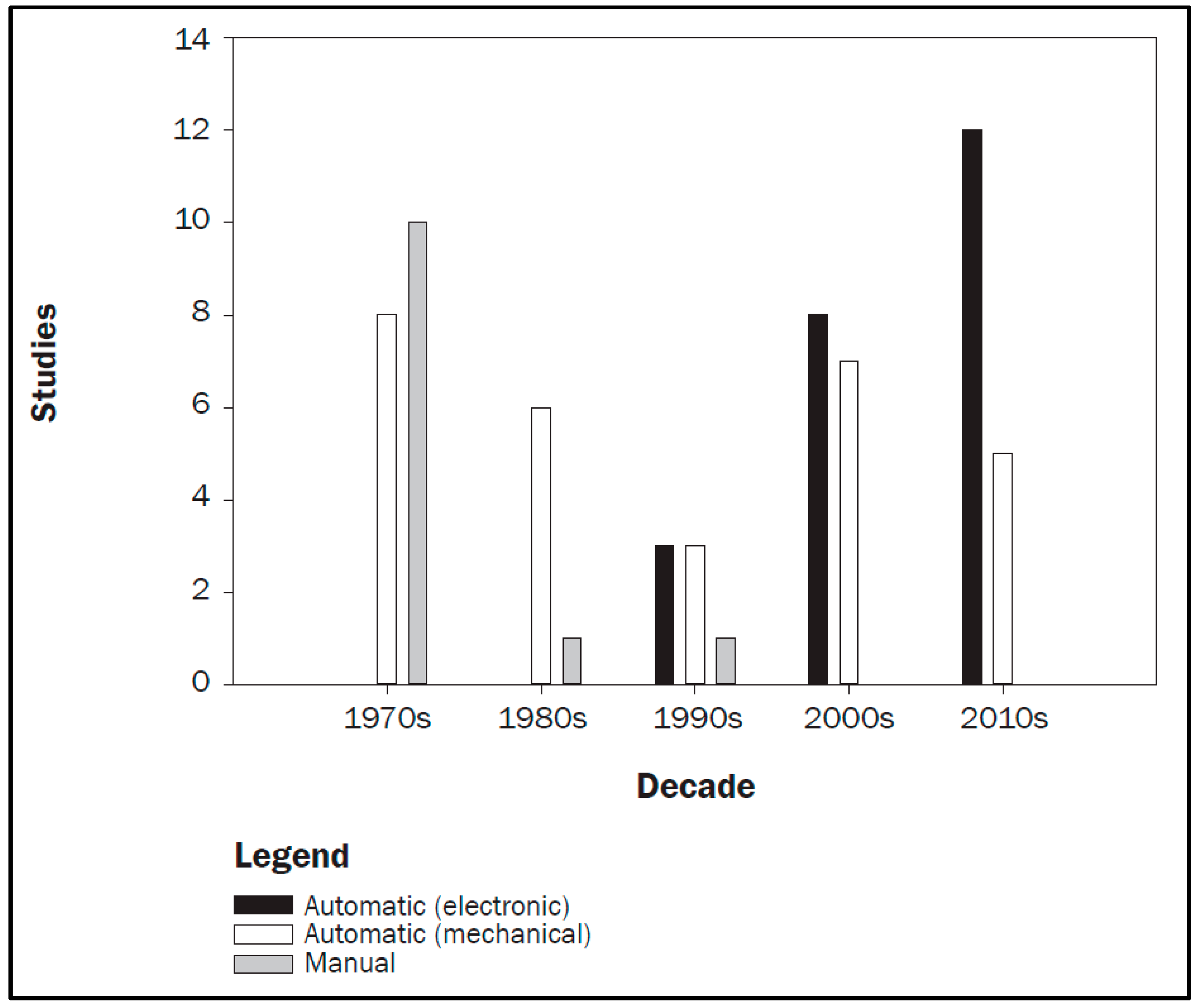
3.3.1. Automated Sampling
| Decision | Annual Cost | Initial (One-Time) Cost | Data Uncertainty | Related Comments |
|---|---|---|---|---|
| How will the constituent concentrations be determined? | Cost estimates below are a function of the project types in Table 1. | - | Carefully consider the following options. | |
| Collect samples to measure the constituent concentrations in the lab | Cost estimates in the following section apply to project types 1, 3, 4. | |||
| Automated sampling with rotating slot or multi-slot divisor mechanical samplers (produces single flow-weighted composite sample and estimates flow volume, thus the discharge measurement options in Table 2 are not needed for load determination). | $/site: maintenance | $-$$/site: mechanical rotating slot or multi-slot sampler (will likely require fabrication) | See [5,12,14] for uncertainty estimates related to automated sampling. | More frequent sampling increases data quality. The unlimited sampling capacity of rotating slot and multi-slot divisor samplers can increase data quality in large events, but they only capture the EMC. Limitation in the size and number of sample bottles in mechanical time-weighted and electronic samplers can decrease data quality in large events, though strategies exist to overcome this [9]. |
| Automated sampling with electronicsamplers | $/site: maintenance | $$/site: electronic sampler | ||
| Lab analysis | $-$$/site: analysis = f (number of samples) | - | See [67,68,69,70,71,72] for Uncertainty estimates related to lab analysis. | Follow sample preservation, storage, and analysis protocols to reduce uncertainty. Estimating the annual number of samples will assist in estimating lab analysis costs [8]. |
| Utilize in situ sensors to measure the constituent concentrations | Cost estimates in the following section apply to project types 2, 5. | See [73,74,75] for additional uncertainty estimates related to in situ sensors. | Avoids lab analysis costs. Provides concentration data with the same time resolution as the flow data. Conduct weekly to biweekly maintenance of the optics. Independently obtain discrete samples for instrument calibration. | |
| $/site: maintenance and calibration | $$$/site: voltametric and amperometric | See [76,77] for nitrate ISE ±0.5 mg N/L for NH4+ [78] | Much of the uncertainty in ISE measurements results from the fouling and drift over time. In situ ISE is currently used only for ammonium > 1 mg N/L. | |
| $$/site: maintenance and calibration | $$$/site: optical UV–VIS spectroscopy and fluorescence sensors | 0.1–12 mg/L NO3-N (±5% +0.2 mg/L) [79] 0–14 mg/L N (±10%) and 0–42 mg/L N (±25%) [80] EXO NitraLED™ ±0.4 mg N/L or 5% (in pure water) | Proxy techniques require a conversion algorithm, but can be highly accurate; subject to interference from water color and turbidity. | |
$$/site: maintenance and calibration | $$$/site: colorimetric sensors with a “lab” onsite | Generally, more accurate than ion specific electrodes, but has smaller range and can require post-correction. | ||
3.3.2. In Situ Sensors
3.4. Decisions with Substantial Impacts on Project Costs and Data Quality
4. Conclusions
Author Contributions
Funding
Data Availability Statement
Acknowledgments
Conflicts of Interest
References
- Harmel, R.; King, K.; Busch, D.; Smith, D.; Birgand, F.; Haggard, B. Measuring edge-of-field water quality: Where we have been and the path forward. J. Soil Water Conserv. 2018, 73, 86–96. [Google Scholar] [CrossRef]
- USDA. Part 600: Introduction. In National Water Quality Handbook; USDA-NRCS: Washington, DC, USA, 1996. [Google Scholar]
- USEPA. Monitoring Guidance for Determining the Effectiveness of Nonpoint-Source Controls; EPA 841-B-96-004; USEPA: Washington, DC, USA, 1997.
- King, K.W.; Harmel, R.D. Comparison of time-based sampling strategies to determine nitrogen loading in plot-scale runoff. Trans. ASAE 2004, 47, 1457–1463. [Google Scholar] [CrossRef]
- King, K.W.; Harmel, R.D. Considerations in selecting a water quality sampling strategy. Trans. ASAE 2003, 46, 63–73. [Google Scholar] [CrossRef]
- Harmel, R.D.; Slade, R.M.; Haney, R.L. Impact of sampling techniques on measured storm water quality data for small streams. J. Environ. Qual. 2010, 39, 1734–1742. [Google Scholar] [CrossRef] [PubMed]
- Harmel, R.D.; King, K.W.; Haggard, B.E.; Wren, D.G.; Sheridan, J.M. Practical guidance for discharge and water quality data collection on small watersheds. Trans. ASABE 2006, 49, 937–948. [Google Scholar] [CrossRef]
- Harmel, R.D.; King, K.W.; Slade, R.M. Automated storm water sampling on small watersheds. Appl. Eng. Agric. 2003, 19, 667–674. [Google Scholar] [CrossRef]
- Gall, H.E.; Jafvert, C.T.; Jenkinson, B. Integrating hydrograph modeling with real-time flow monitoring to generate hydrograph-specific sampling schemes. J. Hydrol. 2010, 393, 331–340. [Google Scholar] [CrossRef]
- Agouridis, C.T.; Edwards, D.R. The development of relationships between constituent concentrations and generic hydrological variables. Trans. ASAE 2003, 46, 245–256. [Google Scholar] [CrossRef]
- King, K.W.; Harmel, R.D.; Fausey, N.R. Development and sensitivity of a method to select time- and flow-paced storm event sampling intervals. J. Soil Water Conserv. 2005, 60, 323–331. [Google Scholar]
- Harmel, R.D.; King, K.W. Uncertainty in measured sediment and nutrient flux in runoff from small agricultural watersheds. Trans. ASAE 2005, 48, 1713–1721. [Google Scholar] [CrossRef]
- Harmel, R.D.; Cooper, R.J.; Slade, R.M.; Haney, R.L.; Arnold, J.G. Cumulative uncertainty in measured streamflow and water quality data for small watersheds. Trans. ASABE 2006, 49, 689–701. [Google Scholar] [CrossRef]
- Miller, P.S.; Mohtar, R.H.; Engel, B.A. Water quality monitoring strategies and their effects on mass load calculation. Trans. ASABE 2007, 50, 817–829. [Google Scholar] [CrossRef]
- USDA-NRCS. Natural Resources Conservation Service, Edge-of-Field Water Quality Monitoring Data Collection and Evaluation—Conservation Activity (Code 201); USDA-NRCS: Washington, DC, USA, 2012.
- USDA-NRCS. Natural Resources Conservation Service, Edge-of-Field Water Quality Monitoring System Installation—Conservation Activity (Code 202); USDA-NRCS: Washington, DC, USA, 2012.
- Jakeman, A.J.; Green, T.R.; Harmel, R.D.; Pembleton, K.; Iwanaga, T. Independent Review of the Paddock to Reef Modelling Program; Queensland Department of Natural Resources, Mines and Energy: Brisbane, Australia, 2019. [Google Scholar]
- Harmel, R.; Hathaway, J.; Wagner, K.; Wolfe, J.; Karthikeyan, R.; Francesconi, W.; McCarthy, D. Uncertainty in monitoring E. coli concentrations in streams and stormwater runoff. J. Hydrol. 2016, 534, 524–533. [Google Scholar] [CrossRef]
- Harmel, R.; Smith, D.; King, K.; Slade, R. Estimating storm discharge and water quality data uncertainty: A software tool for monitoring and modeling applications. Environ. Model. Softw. 2009, 24, 832–842. [Google Scholar] [CrossRef]
- McCarthy, D.; Deletic, A.; Mitchell, V.; Fletcher, T.; Diaper, C. Uncertainties in stormwater E. coli levels. Water Res. 2008, 42, 1812–1824. [Google Scholar] [CrossRef]
- Abtew, W.; Powell, B. Water quality sampling schemes for variable flow canals at remote sites. JAWRA J. Am. Water Resour. Assoc. 2004, 40, 1197–1204. [Google Scholar] [CrossRef]
- Brakensiek, D.L.; Osborn, H.B.; Rawls, W.J. Field Manual for Research in Agricultural Hydrology; Agriculture Handbook, No. 224; USDA: Washington, DC, USA, 1979.
- Buchanan, T.J.; Somers, W.P. Chapter A7: Stage Measurement at Gaging Stations. In Techniques of Water-Resources Investigations of the U.S. Geological Survey, Book 3; USGS: Washington, DC, USA, 1982. [Google Scholar]
- Buchanan, T.J.; Somers, W.P. Chapter A8: Discharge Measurements at Gaging Stations. In Techniques of Water-Resources Investigations of the U.S. Geological Survey, Book 3; USGS: Washington, DC, USA, 1976. [Google Scholar]
- Haan, C.T.; Barfield, B.J.; Hayes, J.C. Design Hydrology and Sedimentology for Small Catchments; Academic Press: New York, NY, USA, 1994. [Google Scholar]
- Kennedy, E.J. Chapter A10: Discharge ratings at gaging stations. In Techniques of Water-Resources Investigations of the U.S. Geological Survey, Book 3; USGS: Washington, DC, USA, 1984. [Google Scholar]
- Carter, R.W.; Davidian, J. Chapter A6: General procedure for gaging streams. In Techniques of Water-Resources Investigations of the U.S. Geological Survey, Book 3; USGS: Washington, DC, USA, 1989. [Google Scholar]
- Birgand, F.; Lellouche, G.; Appelboom, T. Measuring flow in non-ideal conditions for short-term projects: Uncertainties associated with the use of stage-discharge rating curves. J. Hydrol. 2013, 503, 186–195. [Google Scholar] [CrossRef]
- Morlock, S.E.; Nguyen, H.T.; Ross, J.H. Feasibility of Acoustic Doppler Velocity Meters for the Production of Discharge Records from U.S. Geological Survey Streamflow-Gaging Stations; Water-Resources Investigations Report 01-4157; US Geological Survey: Reston, VA, USA, 2002. [CrossRef]
- Birgand, F.; Benoist, J.-C.; Novince, E.; Gilliet, N.; Saint-Cast, P.; Le Saos, E. Flow measurements using ultrasonic Doppler meters in small streams. Ingénieries-EAT 2005, 41, 23–38. (In French) [Google Scholar]
- ISO15769; Hydrometry—Guidelines for the Application of Acoustic Velocity Meters Using the Doppler and Echo Correlation Methods. ISO: Geneva, Switzerland, 2010.
- Stuntebeck, T.D.; Komiskey, M.J.; Owens, D.W.; Hall, D.W. Methods of Data Collection, Sample Processing, and Data Analysis for Edge-of-Field, Streamgaging, Subsurface-Tile, and Meteorological Stations at Discovery Farms and Pioneer Farm in Wisconsin, 2001–2007. US Geol. Surv. Open-File Rep. 2008, 1015, 51. [Google Scholar] [CrossRef]
- Kotlash, A.R.; Chessman, B.C. Effects of water sample preservation and storage on nitrogen and phosphorus determinations: Implications for the use of automated sampling equipment. Water Res. 1998, 32, 3731–3737. [Google Scholar] [CrossRef]
- Harmel, D.; Wagner, K.; Martin, E.; Smith, D.; Wanjugi, P.; Gentry, T.; Gregory, L.; Hendon, T. Effects of field storage method on E. coli concentrations measured in storm water runoff. Environ. Monit. Assess. 2016, 188, 170. [Google Scholar] [CrossRef]
- Holtan, H.N.; Minshall, N.E.; Harrold, L.L. Field Manual for Research in Agricultural Hydrology; Agriculture Handbook, No. 224; Department of Agriculture, Science and Education Administration: Washington, DC, USA, 1962; 215p. [Google Scholar]
- Slade, R.M. General Methods, Information, and Sources for Collecting and Analyzing Water-Resources Data. CD-ROM. Copyright 2004 Raymond M. Slade, Jr. 2004.
- Komiskey, M.J.; Stuntebeck, T.D.; Cox, A.L.; Frame, D.R. Implications of Flume Slope on Discharge Estimates from 0.762-Meter H Flumes Used in Edge-of-Field Monitoring; USGS Open-File Report 2013-1082; US Department of the Interior, US Geological Survey: Reston, VA, USA, 2013. [Google Scholar] [CrossRef]
- Boning, C.W. Policy Statement on Stage Accuracy; Technical Memorandum, No. 93-07; USGS, Office of Water: Washington, DC, USA, 1992.
- Birgand, F.; Benoist, J.; Novince, É.; Gilliet, N.; Saint-Cast, P.; Le Saos, É. Guide for application of continuous Doppler flow meters in wooden trapezoidal flume sections. Ingénieries 2005, 41, 77–82. (In French) [Google Scholar]
- Teledyne ISCO. 2150 Area Velocity Flow Module Datasheet; Teledyne ISCO: Lincoln, Nebraska, 2022. [Google Scholar]
- Tuozzolo, S.; Langhorst, T.; de Moraes Frasson, R.P.; Pavelsky, T.; Durand, M.; Schobelock, J.J. The impact of reach averaging Manning’s equation for an in-situ dataset of water surface elevation, width, and slope. J. Hydrol. 2019, 578, 123866. [Google Scholar] [CrossRef]
- Open Channel Flow Blog. 2023. Available online: www.openchannelflow.com/blog/manning-formula-for-determining-open-channel-flows (accessed on 14 April 2023).
- Maidment, D.R. (Ed.) Handbook of Hydrology; McGraw-Hill: New York, NY, USA, 1993. [Google Scholar]
- Geib, H.V. A new type of installation for measuring soil and water losses from control plots. J. Am. Soc. Agron. 1933, 25, 429–440. [Google Scholar] [CrossRef]
- Edwards, W.M.; Frank, H.E.; King, T.E.; Gallwitz, D.R. Runoff Sampling: Coshocton Vane Proportional Sampler; Pub. No. ARS-NC-50; USDA-ARS: Washington, DC, USA, 1976.
- Parsons, D.A. Coshocton-Type Runoff Samplers; ARS-41-2; USDA-ARS: Washington, DC, USA, 1955.
- Parsons, D.A. Coshocton-Type Runoff Samplers: Laboratory Investigations; SCS-TP-124; USDA-ARS: Washington, DC, USA, 1954.
- Allen, P.B.; Welch, N.H.; Rhoades, E.D.; Edens, C.D.; Miller, G.E. The Modified Chickasha Sediment Sampler; Pub. No. ARS-S-107; USDA-ARS: Washington, DC, USA, 1976.
- Kirchner, J.W.; Feng, X.; Neal, C.; Robson, A.J. The fine structure of water-quality dynamics: The (high-frequency) wave of the future. Hydrol. Process. 2004, 18, 1353–1359. [Google Scholar] [CrossRef]
- Martin, G.R.; Smoot, J.L.; White, K.D. A comparison of surface-grab and cross sectionally integrated stream-water-quality sampling methods. Water Environ. Res. 1992, 64, 866–876. [Google Scholar] [CrossRef]
- Ging, P.B. Water-Quality Assessment of South-Central Texas—Comparison of Water Quality in Surface-Water Samples Collected Manually and by Automated Samplers; USGS Fact Sheet FS-172-99; US Department of the Interior, US Geological Survey: Reston, VA, USA, 1999. [CrossRef]
- Wilde, F.D.; Radtke, D.B. Chapter A6: Field measurements: General information and guidelines. In Techniques of Water-Resources Investigations of the U.S. Geological Survey, Book 9; USGS: Washington, DC, USA, 2005. [Google Scholar]
- Wells, F.; Gibbons, W.; Dorsey, M. Guidelines for Collection and Field Analysis of Water-Quality Samples from Streams in Texas; USGS Open-File Report 90-127; USGS: Austin, TX, USA, 1990.
- USGS. Handbooks for Water-Resources Investigations, Section A. National Field Manual for Collection of Water-Quality Data. In Techniques of Water-Resources Investigations of the United States Geological Survey, Book 9; US Department of the Interior, US Geological Survey: Reston, VA, USA, 1999. [Google Scholar]
- Bonta, J.V. Modification and performance of the Coshocton wheel with the modified drop-box weir. J. Soil Water Conserv. 2002, 57, 364–373. [Google Scholar]
- Bonta, J.V. Water sampler and flow measurement for runoff containing large sediment particles. Trans. ASAE 1999, 42, 107–114. [Google Scholar] [CrossRef]
- Malone, R.W.; Bonta, J.V.; Lightell, D. A low-cost composite water sampler for drip and stream flow. Appl. Eng. Agric. 2003, 19, 59–61. [Google Scholar] [CrossRef]
- Sheridan, J.M.; Lowrance, R.R.; Henry, H.H. Surface flow sampler for riparian studies. Appl. Eng. Agric. 1996, 12, 183–188. [Google Scholar] [CrossRef]
- Pinson, W.T.; Yoder, D.C.; Buchanan, J.R.; Wright, W.C.; Wilkerson, J.B. Design and evaluation of an improved flow divider for sampling runoff plots. Appl. Eng. Agric. 2004, 20, 433–437. [Google Scholar] [CrossRef]
- Franklin, D.H.; Cabrera, M.L.; Steiner, J.L.; Endale, D.M.; Miller, W.P. Evaluation of percent flow captured by a small in-field runoff collector. Trans. ASAE 2001, 44, 551–554. [Google Scholar] [CrossRef]
- Inter-Agency Committee on Water Resources, Subcommittee on Sedimentation, ICRW-SS. The Single-Stage Sampler for Suspended Sediment; Report 13; St. Anthony Falls Hydraulics Laboratory: Minneapolis, MN, USA, 1961; 105p.
- Edwards, T.K.; Glysson, G.D. Field Methods for Measurement of Fluvial Sediment: U.S. Geological Survey Open-File Report 86-531; US Department of the Interior, US Geological Survey: Reston, VA, USA, 1988; 118p.
- Graczyk, D.J.; Robertson, D.M.; Rose, W.J.; Steur, J.J. Comparison of Water-Quality Samples Collected by Siphon Samplers and Automatic Samplers in Wisconsin; USGS Fact Sheet FS-067-00; US Geological Survey: Reston, VA, USA, 2000. [CrossRef]
- Richards, R.P.; Holloway, J. Monte Carlo studies of sampling strategies for estimating tributary loads. Water Resour. Res. 1987, 23, 1939–1948. [Google Scholar] [CrossRef]
- Leecaster, M.K.; Schiff, K.; Tiefenthaler, L.L. Assessment of efficient sampling designs for urban stormwater monitoring. Water Res. 2002, 36, 1556–1564. [Google Scholar] [CrossRef]
- Veith, T.; Preisendanz, H.; Elkin, K. Characterizing transport of natural and anthropogenic constituents in a long-term agricultural watershed in the northeastern United States. J. Soil Water Conserv. 2020, 75, 319–329. [Google Scholar] [CrossRef]
- Gordon, J.D.; Newland, C.A.; Gagliardi, S.T. Laboratory Performance in the Sediment Laboratory Quality-Assurance Project, 1996–1998; USGS Water Resources Investigations Report 99-4184; US Department of the Interior, US Geological Survey: Reston, VA, USA, 2000. [CrossRef]
- Miller, R.O.; Kotuby-Amacher, J. North American Proficiency Testing (NAPT) Program; Colorado State University: Fort Collins, CO, USA; Utah State University: Logan, UT, USA, 2005; unpublished data. [Google Scholar]
- Mercurio, G.; Perot, J.; Roth, N.; Southerland, M. Maryland Biological Stream Survey 2000: Quality Assessment Report; Versar, Inc.: Springfield, VA, USA; Maryland Department of Natural Resources: Baltimore, MD, USA, 2002. [Google Scholar]
- Ludtke, A.S.; Woodworth, M.T.; Marsh, P.S. Quality Assurance Results for Routine Water Analysis in U.S. Geological Survey Laboratories, Water Year 1998; USGS Water Resources Investigations Report 00-4176; USGS: Washington, DC, USA, 2000.
- USEPA. Method 1603: Escherichia coli (E. coli) in Water by Membrane Filtration Using Modified Membrane-Thermotolerant Escherichia coli Agar (Modified mTEC); EPA-821-R-06-011; Environmental Protection Agency, Office of Water: Washington, DC, USA, 2006.
- USEPA. Results of the Interlaboratory Testing Study for the Comparison of Methods for Detection and Enumeration of Enterococci and Escherichia coli in Combined Sewer Overflows (CSOs); EPA-821-R-08-006; Environmental Protection Agency, Office of Water: Washington, DC, USA, 2008.
- Johengen, T.; Purcell, H.; Tamburri, M.; Loewensteiner, D.; Smith, G.J.; Schar, D.; McManus, M.; Walker, G. Performance Verification Statement for Sea-Bird Scientific HydroCycle Phosphate Analyzer; Alliance for Coastal Technologies (ACT): Solomons, MD, USA, 2017. [Google Scholar] [CrossRef]
- Blaen, P.J.; Khamis, K.; Lloyd, C.E.; Bradley, C.; Hannah, D.; Krause, S. Real-time monitoring of nutrients and dissolved organic matter in rivers: Capturing event dynamics, technological opportunities and future directions. Sci. Total Environ. 2016, 569–570, 647–660. [Google Scholar] [CrossRef]
- Snazelle, T. Laboratory Evaluation of the Sea-Bird Scientific HydroCycle-PO4 Phosphate Sensor. 2018. Available online: https://pubs.usgs.gov/of/2018/1120/ofr20181120.pdf (accessed on 14 April 2023).
- Le Goff, T.; Braven, J.; Ebdon, L.; Scholefield, D. Automatic continuous river monitoring of nitrate using a novel ion-selective electrode. J. Environ. Monit. 2003, 5, 353–358. [Google Scholar] [CrossRef]
- Le Goff, T.; Braven, J.; Ebdon, L.; Chilcott, N.P.; Scholefield, D.; Wood, J.W. An accurate and stable nitrate-selective electrode for the in situ determination of nitrate in agricultural drainage waters. Analyst 2002, 127, 507–511. [Google Scholar] [CrossRef]
- S::CAN. Jianshan Waste Water Treatment Plant Controls the Nitrogen Removal Process and Optimizes the Carbon Source Dosage. 2017. Available online: www.s-can.at/wp_contents/uploads/2021/09/reference_jianshan_wwtp_cn_en_2017_11_web.pdf (accessed on 14 April 2023).
- OTT. Technical Data OTT ecoN; V-06/02/2019; OTT Hydromet GmbH: Kempten, Germany, 2019. [Google Scholar]
- OTT. Technical Data Sea-Bird Scientific SUNA Optical Nitrate Sensor; V-06/02/2019; OTT Hydromet GmbH: Kempten, Germany, 2019. [Google Scholar]
- Williams, M.R.; King, K.W.; Macrae, M.L.; Ford, W.; Van Esbroeck, C.; Brunke, R.I.; English, M.C.; Schiff, S.L. Uncertainty in nutrient loads from tile-drained landscapes: Effect of sampling frequency, calculation algorithm, and compositing strategy. J. Hydrol. 2015, 530, 306–316. [Google Scholar] [CrossRef]
- Mentz, R.S.; Busch, D.L.; Ribikawskis, M.; VanRyswyk, W.S.; Tomer, M.D. Monitoring Edge-of-Field Surface-Water Runoff: A Three-State Pilot Project to Promote and Evaluate a Simple, Inexpensive, and Reliable Gauge; USDA Natural Resources Conservation Service Final Project Report; USDA: Washington, DC, USA, 2016.
- Ham, J.; Wardle, E. Next Generation Technology for Monitoring Edge-of-Field Water Quality in Organic Agriculture; USDA-NRCS CIG Final Report; Colorado State University, Department of Soil and Crop Sciences: Washington, DC, USA, 2022. [Google Scholar]
- Rode, M.; Wade, A.J.; Cohen, M.J.; Hensley, R.T.; Bowes, M.J.; Kirchner, J.W.; Arhonditsis, G.B.; Jordan, P.; Kronvang, B.; Halliday, S.J.; et al. Sensors in the stream: The high-frequency wave of the present. Environ. Sci. Technol. 2016, 50, 10297–10307. [Google Scholar] [CrossRef]
- Pellerin, B.A.; Stauffer, B.A.; Young, D.A.; Sullivan, D.J.; Bricker, S.B.; Walbridge, M.R.; Clyde, G.A., Jr.; Shaw, D.M. Emerging tools for continuous nutrient monitoring networks: Sensors advancing science and water resources protection. J. Am. Water Resour. Assoc. 2016, 52, 993–1008. [Google Scholar] [CrossRef]
- Burns, D.A.; Pellerin, B.A.; Miller, M.P.; Capel, P.D.; Tesoriero, A.J.; Duncan, J.M. Monitoring the riverine pulse: Applying high-frequency nitrate data to advance integrative understanding of biogeochemical and hydrological processes. WIREs Water 2019, 6, e1348. [Google Scholar] [CrossRef]
- Erwin, E.G.; McLaughlin, D.L.; Stewart, R.D. Installation matters: Implications for in situ water quality monitoring. Water Resour. Res. 2021, 57, e2020WR028294. [Google Scholar] [CrossRef]
- Hanrahan, G.; Patil, D.G.; Wang, J. Electrochemical sensors for environmental monitoring: Design, development and applications. J. Environ. Monit. 2004, 6, 657–664. [Google Scholar] [CrossRef] [PubMed]
- Scholefield, D.; Stone, A.C.; Braven, J.; Chilcott, N.P.; Ebdon, L.; Sutton, P.G.; Wood, J.W. Field evaluation of a novel nitrate sensitive electrode in drainage waters from agricultural grassland. Analyst 1999, 124, 1467–1470. [Google Scholar] [CrossRef]
- Etheridge, J.R.; Birgand, F.; Burchell, M.R.; Smith, B.T. Addressing the fouling of in situ ultraviolet-visual spectrometers used to continuously monitor water quality in brackish tidal marsh waters. J. Environ. Qual. 2013, 42, 1896–1901. [Google Scholar] [CrossRef]
- Lenhart, C.F.; Brooks, K.N.; Heneley, D.; Magner, J.A. Spatial and temporal variation in suspended sediment, organic matter, and turbidity in a Minnesota prairie river: Implications for TMDLs. Environ. Monit. Assess. 2009, 165, 435–447. [Google Scholar] [CrossRef]
- Jones, A.S.; Horsburgh, J.S.; Mesner, N.O.; Ryel, R.J.; Stevens, D.K. Influence of sampling frequency on estimation of annual total phosphorus and total suspended solids loads. JAWRA J. Am. Water Resour. Assoc. 2012, 48, 1258–1275. [Google Scholar] [CrossRef]
- Grayson, R.; Finlayson, B.; Gippel, C.; Hart, B. The potential of field turbidity measurements for the computation of total phosphorus and suspended solids loads. J. Environ. Manag. 1996, 47, 257–267. [Google Scholar] [CrossRef]
- Gippel, C.J. Potential of turbidity monitoring for measuring the transport of suspended solids in streams. Hydrol. Process. 1995, 9, 83–97. [Google Scholar] [CrossRef]
- Saraceno, J.F.; Pellerin, B.A.; Downing, B.D.; Boss, E.; Bachand, P.A.M.; Bergamaschi, B.A. High-frequency in situ optical measurements during a storm event: Assessing relationships between dissolved organic matter, sediment concentrations, and hydrologic processes. J. Geophys. Res. Atmos. 2009, 114, G00F09. [Google Scholar] [CrossRef]
- Moin, S. Evaluating the Benefits of Near-continuous Monitoring, Real-Time Control, and SCM Visibility in Performance of Stormwater Control Measures. Ph.D. Dissertation, North Carolina State University, Raleigh, NC, USA, 2021. [Google Scholar]
- Birgand, F.; Lefrançois, J.; Grimaldi, C.; Novince, E.; Gilliet, N.; Gascuel-Odoux, C. Flux measurement and sampling of total suspended solids in small agricultural streams. Ingénieries–EAT 2004, 40, 21–35. (In French) [Google Scholar]
- Birgand, F.; Aveni-Deforge, K.; Smith, B.; Maxwell, B.; Horstman, M.; Gerling, A.B.; Carey, C.C. First report of a novel multiplexer pumping system coupled to a water quality probe to collect high temporal frequency in situ water chemistry measurements at multiple sites. Limnol. Oceanogr. Methods 2016, 14, 767–783. [Google Scholar] [CrossRef]
- Minella, J.P.G.; Merten, G.H.; Reichert, J.M.; Clarke, R.T. Estimating suspended sediment concentrations from turbidity measurements and the calibration problem. Hydrol. Process. 2007, 22, 1819–1830. [Google Scholar] [CrossRef]
- Jones, A.S.; Stevens, D.K.; Horsburgh, J.S.; Mesner, N.O. Surrogate measures for providing high frequency estimates of total suspended solids and total phosphorus Concentrations1. JAWRA J. Am. Water Resour. Assoc. 2010, 47, 239–253. [Google Scholar] [CrossRef]
- Navratil, O.; Esteves, M.; Legout, C.; Gratiot, N.; Nemery, J.; Willmore, S.; Grangeon, T. Global uncertainty analysis of suspended sediment monitoring using turbidimeter in a small mountainous river catchment. J. Hydrol. 2011, 398, 246–259. [Google Scholar] [CrossRef]
- Thompson, J.; Cassidy, R.; Doody, D.G.; Flynn, R. Assessing suspended sediment dynamics in relation to ecological thresholds and sampling strategies in two Irish headwater catchments. Sci. Total Environ. 2014, 468–469, 345–357. [Google Scholar] [CrossRef] [PubMed]
- Etheridge, J.R.; Birgand, F.; Osborne, J.A.; Osburn, C.L.; Burchell, M.R.; Irving, J. Using in situ ultraviolet-visual spectroscopy to measure nitrogen, carbon, phosphorus, and suspended solids concentrations at a high frequency in a brackish tidal marsh. Limnol. Oceanogr. Methods 2014, 12, 10–22. [Google Scholar] [CrossRef]
- Khamis, K.; Sorensen, J.P.R.; Bradley, C.; Hannah, D.M.; Lapworth, D.J.; Stevens, R. In situ tryptophan-like fluorometers: Assessing turbidity and temperature effects for freshwater applications. Environ. Sci. Process. Impacts 2015, 17, 740–752. [Google Scholar] [CrossRef] [PubMed]
- Tzortziou, M.; Neale, P.J.; Osburn, C.L.; Megonigal, J.P.; Maie, N.; Jaffé, R. Tidal marshes as a source of optically and chemically distinctive colored dissolved organic matter in the Chesapeake Bay. Limnol. Oceanogr. 2008, 53, 148–159. [Google Scholar] [CrossRef]
- Osburn, C.L.; Wigdahl, C.R.; Fritz, S.C.; Saros, J.E. Dissolved organic matter composition and photoreactivity in prairie lakes of the U.S. Great Plains. Limnol. Oceanogr. 2011, 56, 2371–2390. [Google Scholar] [CrossRef]
- Osburn, C.L.; Mikan, M.P.; Etheridge, J.R.; Burchell, M.R.; Birgand, F. Seasonal variation in the quality of dissolved and particulate organic matter exchanged between a salt marsh and its adjacent estuary. J. Geophys. Res. Biogeosci. 2015, 120, 1430–1449. [Google Scholar] [CrossRef]
- Osburn, C.L.; Handsel, L.T.; Peierls, B.L.; Paerl, H.W. Predicting sources of dissolved organic nitrogen to an estuary from an agro-urban coastal watershed. Environ. Sci. Technol. 2016, 50, 8473–8484. [Google Scholar] [CrossRef] [PubMed]
- Bedell, E.; Harmon, O.; Frankhauser, K.; Shivers, Z.; Thomas, E. A continuous, in-situ, near-time fluorescence sensor coupled with a machine learning model for detection of fecal contamination in drinking water: Design, characterization, and field validation. Water Res. 2022, 220, 118644. [Google Scholar] [CrossRef]
- Dialameh, B.; Ghane, E. Effect of water sampling strategies on the uncertainty of phosphorus load estimation in subsurface drainage discharge. J. Environ. Qual. 2022, 51, 377–388. [Google Scholar] [CrossRef]
- Cassidy, R.; Jordan, P. Limitations of instantaneous water quality sampling in surface-water catchments: Comparison with near-continuous phosphorus time-series data. J. Hydrol. 2011, 405, 182–193. [Google Scholar] [CrossRef]
- Zhang, J.; Zhang, C. Quality assurance/quality control in surface water sampling. In Quality Assurance and Quality Control of Environmental Field Sampling; Zhang, C., Mueller, J.F., Mortimer, M.R., Eds.; Future Science: London, UK, 2014. [Google Scholar]
- Harmel, R.; Smith, P.; Migliaccio, K.; Chaubey, I.; Douglas-Mankin, K.; Benham, B.; Shukla, S.; Muñoz-Carpena, R.; Robson, B. Evaluating, interpreting, and communicating performance of hydrologic/water quality models considering intended use: A review and recommendations. Environ. Model. Softw. 2014, 57, 40–51. [Google Scholar] [CrossRef]
- Daniels, M.; Sharpley, A.; Harmel, R.; Anderson, K. The utilization of edge-of-field monitoring of agricultural runoff in addressing nonpoint source pollution. J. Soil Water Conserv. 2018, 73, 1–8. [Google Scholar] [CrossRef]
- Montgomery, R.H.; Sanders, T.G. Uncertainty in water quality d57ata. Dev. Water Sci. 1986, 27, 17–29. [Google Scholar] [CrossRef]

| Project Type | Data Measured | Discharge Measurement | Sample Collection | Lab Analysis |
|---|---|---|---|---|
| 1. Measure concentrations with electronic samplers and subsequent lab analysis | Concentrations | NA |  | |
| 2. Measure concentrations with in situ sensors | Concentrations | NA | NA | NA |
| 3. Measure concentrations and loads with mechanical rotating slot or multi-slot samplers and subsequent lab analysis | Concentrations and loads | | | |
| 4. Measure concentrations and loads with electronic samplers and subsequent lab analysis | Concentrations and loads | | | |
| 5. Measure concentrations and loads with in situ sensors | Concentrations and loads | | NA | NA |
| Item(s) for Initial Purchase | Initial Cost | Item(s) with Annual Cost | Annual Cost | |
|---|---|---|---|---|
| All projects | ||||
| Number of sites | Vehicle | USD 50,000 | Technical staff salary | USD 100,000 |
| Location of sites | Installation = f (berm construction) | USD 800-16,000 | Site maintenance; travel costs = f (location, proximity) | USD 3400–6000 |
| Equipment shelter | Shelter = f (commercial or homemade/repurposed) | USD 2400–8000 | - | - |
| Duplicate equipment (included in cost below based on equipment type) | Backup/replacement equipment set (per every 6–10 sites) | - | - | - |
| Power (for electronic samplers and in situ sensors) | Electrical = f (battery; solar or electrical power) | USD 3200–23,200 | Electricity use (maintain and recharge batteries) | USD 960 |
| Communication device (for electronic samplers and in situ sensors) | Communication = f (device needed) | USD 0–1200 | Fees = f (data plan requirements) | USD 0–1440 |
| 1. Projects that measure concentrations with electronic samplers and subsequent lab analysis | ||||
| Collect samples | Sampler | USD 54,000 | Equipment maintenance = f (sampler type) | USD 960 |
| Conduct lab analysis | - | - | Sample analysis = f (discrete or composite samples) | USD 4000– 40,000 |
| Initial cost = USD 110,400–152,400 Annual cost = USD 109,320–149,360 Total (3 yr) project cost = USD 438,360–600,480 | ||||
| 2. Projects that measure concentrations with in situ sensors | ||||
| Determine concentrations | Sensor = f (sensor type) | USD 135,000–USD 180,000 | Equipment maintenance and calibration | USD 5000–USD 15,000 |
| Initial cost = USD 191,400–258,400 Annual cost = USD 109,360–123,400 Total (3 yr) project cost = USD 519,480–628,600 | ||||
| 3. Projects that measure concentrations and loads with rotating slot or multi-slot samplers and subsequent lab analysis | ||||
| Collect composite sample | Sampler | USD 6750 | Equipment maintenance | USD 480 |
| Conduct lab analysis | - | - | Sample analysis | USD 4000 |
| Initial cost = USD 59,950–80,750 Annual cost = USD 107,880–110,480 Total (3 yr) project cost = USD 383,590–412,190 | ||||
| 4. Projects that measure concentrations and loads with electronic samplers and subsequent lab analysis | ||||
| Collect samples | Sampler | USD 54,000 | Equipment maintenance | USD 960 |
| Conduct lab analysis | - | - | Sample analysis = f (discrete or composite samples) | USD 4000–40,000 |
| Measure discharge volume | Equipment = f (control structure, stage/flow measurement) | USD 9000–57,000 | Equipment maintenance; measurement = f (stage– discharge relationship) | USD 0–3200 |
| Initial cost = USD 119,400–209,200 Annual cost = USD 109,320–152,560 Total (3 yr) project cost = USD 447,360–667,080 | ||||
| 5. Projects that measure concentrations and loads with in situ sensors | ||||
| Determine concentrations | Sensor = f (sensor type) | USD 135,000– 180,000 | Equipment maintenance and calibration | USD 5000–15,000 |
| Measure discharge volume | Equipment = f (control structure, stage/flow measurement) | USD 9000– 57,000 | Equipment maintenance; measurement = f (stage– discharge relationship) | USD 0–3200 |
| Initial cost = USD 200,400–315,400 Annual cost = USD 109,360–126,600 Total (3 yr) project cost = USD 528,480–695,200 | ||||
Disclaimer/Publisher’s Note: The statements, opinions and data contained in all publications are solely those of the individual author(s) and contributor(s) and not of MDPI and/or the editor(s). MDPI and/or the editor(s) disclaim responsibility for any injury to people or property resulting from any ideas, methods, instructions or products referred to in the content. |
© 2023 by the authors. Licensee MDPI, Basel, Switzerland. This article is an open access article distributed under the terms and conditions of the Creative Commons Attribution (CC BY) license (https://creativecommons.org/licenses/by/4.0/).
Share and Cite
Harmel, R.D.; Preisendanz, H.E.; King, K.W.; Busch, D.; Birgand, F.; Sahoo, D. A Review of Data Quality and Cost Considerations for Water Quality Monitoring at the Field Scale and in Small Watersheds. Water 2023, 15, 3110. https://doi.org/10.3390/w15173110
Harmel RD, Preisendanz HE, King KW, Busch D, Birgand F, Sahoo D. A Review of Data Quality and Cost Considerations for Water Quality Monitoring at the Field Scale and in Small Watersheds. Water. 2023; 15(17):3110. https://doi.org/10.3390/w15173110
Chicago/Turabian StyleHarmel, Robert Daren, Heather Elise Preisendanz, Kevin Wayne King, Dennis Busch, Francois Birgand, and Debabrata Sahoo. 2023. "A Review of Data Quality and Cost Considerations for Water Quality Monitoring at the Field Scale and in Small Watersheds" Water 15, no. 17: 3110. https://doi.org/10.3390/w15173110
APA StyleHarmel, R. D., Preisendanz, H. E., King, K. W., Busch, D., Birgand, F., & Sahoo, D. (2023). A Review of Data Quality and Cost Considerations for Water Quality Monitoring at the Field Scale and in Small Watersheds. Water, 15(17), 3110. https://doi.org/10.3390/w15173110