Enhancing Water Temperature Prediction in Stratified Reservoirs: A Process-Guided Deep Learning Approach

Abstract

Data-driven models (DDMs) are extensively used in environmental modeling yet encounter obstacles stemming from limited training data and potential discrepancies with physical laws. To address this challenge, this study developed a process-guided deep learning (PGDL) model, integrating a long short-term memory (LSTM) neural network and a process-based model (PBM), CE-QUAL-W2 (W2), to predict water temperature in a stratified reservoir. The PGDL model incorporates an energy constraint term derived from W2′s thermal energy equilibrium into the LSTM’s cost function, alongside the mean square error term. Through this mechanism, PGDL optimizes parameters while penalizing deviations from the energy law, thereby ensuring adherence to crucial physical constraints. In comparison to LSTM’s root mean square error (RMSE) of 0.062 °C, PGDL exhibits a noteworthy 1.5-fold enhancement in water temperature prediction (RMSE of 0.042 °C), coupled with improved satisfaction in maintaining energy balance. Intriguingly, even with training on just 20% of field data, PGDL (RMSE of 0.078 °C) outperforms both LSTM (RMSE of 0.131 °C) and calibrated W2 (RMSE of 1.781 °C) following pre-training with 80% of the data generated by the uncalibrated W2 model. The successful integration of the PBM and DDM in the PGDL validates a novel technique that capitalizes on the strengths of multidimensional mathematical models and data-based deep learning models. Furthermore, the pre-training of PGDL with PBM data demonstrates a highly effective strategy for mitigating bias and variance arising from insufficient field measurement data.

1. Introduction

Process-based (PB) hydrodynamics and water quality models such as CE-QUAL-W2 (W2) [1], environmental fluid dynamics code (EFDC) [2], and aquatic ecology model 3D (AEM3D) [3] are effective tools for studying temperature dynamics and heat transfer in surface water. Nevertheless, these models are accompanied by several drawbacks pertaining to substantial data prerequisites, the challenge of parameter calibration, inherent model uncertainties, demanding computational requirements, and the need for specialized expertise. These limitations collectively constrain their practical utility and accuracy [4,5,6].

In recent years, the rapid advancements in data science technology have led to a significant increase in the utilization of data-driven models (DDMs) across various domains [7,8,9,10]. These innovative machine learning (ML) algorithms have expanded beyond their traditional role as scientific analytical tools and become integral components in fields like medicine, life sciences, and meteorology [11,12]. The water environment domain is no exception, with a growing demand for DDMs to enhance predictive performance and optimize the utility of monitoring data [13,14,15]. Notably, recent publications in water environment modeling revealed an interesting trend: since 2010, DDMs have become more prevalent than process-based models (PBMs) [16].

Compared to PBMs, DDMs can interpret data patterns and relationships without prior knowledge of the phenomenon. They offer a simpler structure, faster calculation, and excellent predictive performance [17,18]. Additionally, DDM allows easy quantification of model sensitivity and uncertainty, addressing a limitation of PBM [19,20,21]. However, despite their excellent predictive performance, DDM can suffer from poor interpretation of results due to overfitting and may not perform well with limited, high-quality data [22,23]. Another limitation of DDM is its failure to consider classical energy, mass, and momentum conservation principles, resulting in predictions that do not capture the dynamic relationship between water quality kinetics, hydrodynamics, and ecological processes in real systems [24,25].

To leverage the strengths of PBMs and DDMs while addressing their limitations, the development of a technology that combines the two models becomes necessary. Thus, a “theory-guided” hybrid framework was developed and employed. Theory-guided data science (TGDS) represents a novel modeling paradigm that integrates scientific knowledge and mechanical principles to enhance the effectiveness of DDMs for understanding and predicting various issues arising from direct and indirect human activities [26]. These models enable achieving consistency in outcomes by incorporating scientific data as a critical component, along with training accuracy and model complexity, which balance the bias and variance errors that commonly occur in generalized DDMs. Additionally, TGDS enables the identification and elimination of inconsistencies through the application of scientific knowledge, leading to a significant reduction in variance without affecting model bias [27,28].

The applicability of TGDS extends to numerous scientific domains due to its effectiveness in addressing problems in fields such as biomedical science [29,30], hydrology [31,32], climatology [33], quantum chemistry [34], and biomarker discovery [35]. Karpatne et al. [26] introduced a TGDS model design that encompassed learning methods, data refinement, and model structure across five specific areas: turbulence modeling, hydrology, computational chemistry, mapping of water surface dynamics, and postprocessing using elevation constraints. Furthermore, TGDS has applications in other areas such as civil engineering and geology [36], aerodynamics [37], fluid dynamics [38], and physics [39,40,41].

The application of TGDS is gaining traction in the realm of aquatic environments. Karpatne et al. [26] employed physics-guided neural networks to predict lake water temperature, considering empirical and structural errors and ensuring physical consistency within the DDM. Noori et al. [42,43] utilized dimension reduction models to predict water temperature variations over time and depth in Karkheh Dam (Iran). This was accomplished by integrating the W2 model with proper orthogonal decomposition, enhancing the interpretation of simulated water temperature patterns within reservoirs. Read et al. [24] predicted water temperature over time and depth in stratified lakes by combining the General Lake Model (GLM), a one-dimensional lake model based on dynamical theory, with a recurrent neural network (RNN) model. Hanson et al. [44] utilized a simple box-type phosphorus mass balance model in conjunction with an RNN to forecast phosphorus concentration in Lake Mendota, located in Wisconsin, USA.

Although notable efforts have been made to develop and utilize TGDS in aquatic environments, a critical research gap exists within the context of aquatic environments. While TGDS offer exceptional predictive capabilities and efficiency, their application to complex water bodies with substantial spatial variations in temperature and water quality, such as large dam reservoirs, remains underexplored. Existing TGDS often rely on simplified zero- or one-dimensional dynamic models, limiting their accuracy and applicability in such intricate settings. This gap underscores the necessity for research that bridges this divide by integrating multidimensional PBMs and DDMs, enabling a more comprehensive and accurate understanding of water temperature dynamics in these challenging environments. The current study addresses this pressing research gap by developing a novel process-guided deep learning (PGDL) model that combines the strengths of both PBMs and DDMs to predict water temperatures in the Daecheong Reservoir, thereby offering a pivotal contribution towards enhancing our predictive capabilities and management strategies in complex aquatic systems.

Consequently, the objective of this study was to develop a PGDL model that integrates a long short-term memory (LSTM) [45] model with a two-dimensional process-based (PB) mechanistic model, W2 [1,46,47], to predict longitudinal and vertical water temperatures in the Daecheong Reservoir located in the temperate zone of the Republic of Korea. Furthermore, the study aimed to evaluate the predictive performance of the model in terms of satisfying the energy conservation law. The LSTM and W2 models were trained and calibrated individually using water temperature data and meteorological data collected from a thermistor chain in the Daecheong Reservoir between July 2017 and December 2018. To combine the two models, the PGDL model was trained by incorporating a penalty into the loss function of the LSTM model to address any violations of the energy balance. For different seasons and water depths, the accuracy of water temperature prediction for each model was assessed by comparing the errors against actual values, and thus, the satisfaction of the energy conservation law was evaluated. Furthermore, to examine the impact of the amount of measured data required for training, the performance of water temperature prediction was compared using a pre-training technique that utilized the uncalibrated results of the W2 model as training data.

The novelty of this study lies in its response to a crucial research gap in the field of aquatic environment modeling. While DDMs and PBMs have made significant advancements, their integration in this context remains underexplored. This study demonstrates the applicability of a novel modeling approach that integrates a deep learning model with a multidimensional PBM. Moreover, the findings highlighted the effectiveness of utilizing PBMs to generate essential training data for the development of deep learning models. The results contribute to enhancing predictive capabilities and management strategies in complex aquatic systems, demonstrating the effectiveness of this innovative integration.

2. Materials and Methods

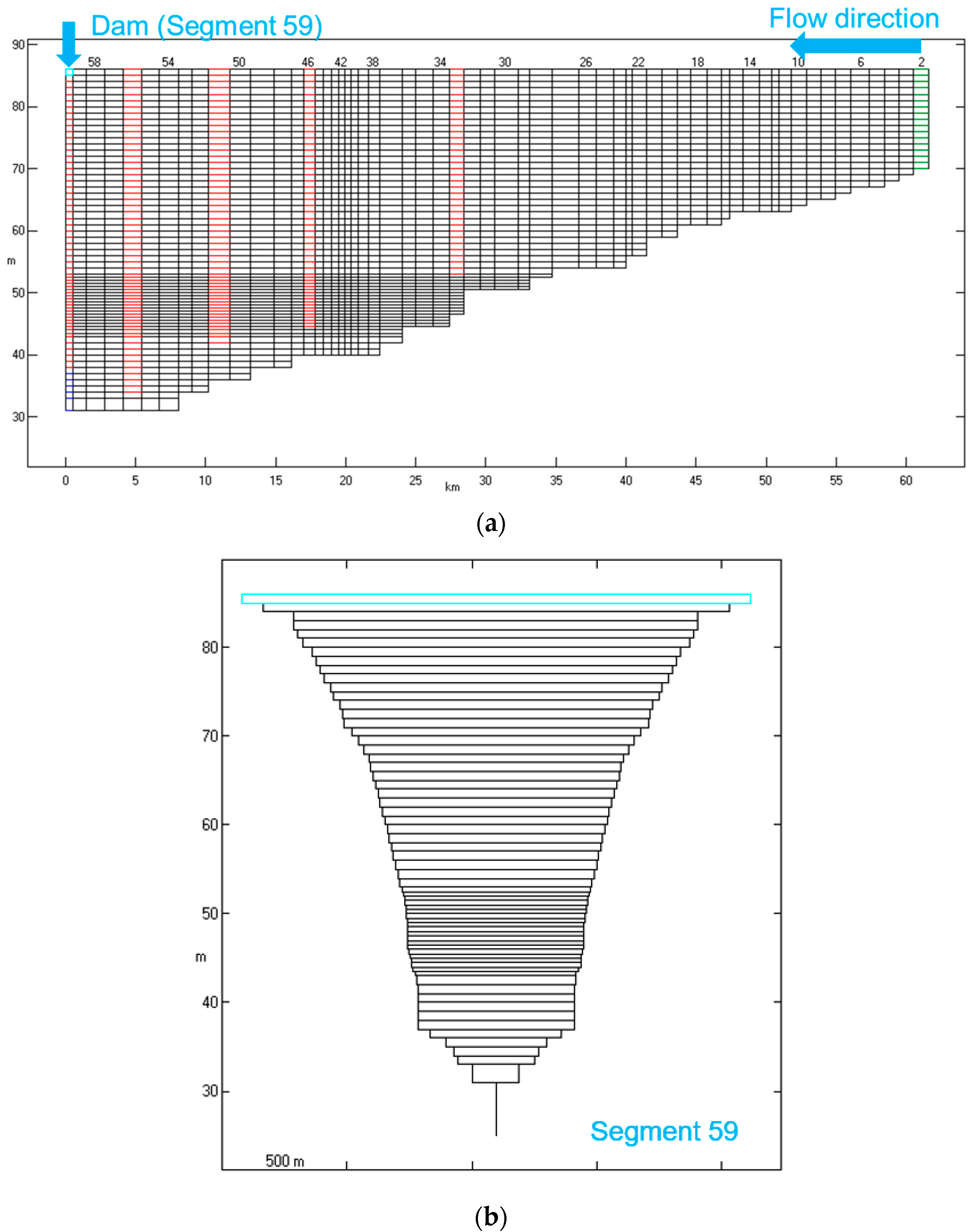
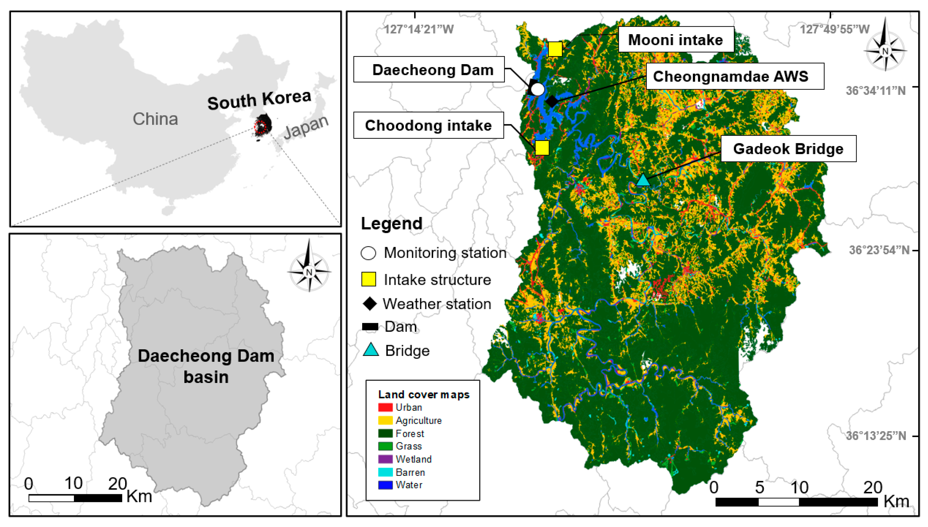
2.1. Description of the Site

In this study, the Daecheong Reservoir was selected as the modeling target, which is located in the Geum River, one of the four major rivers in Korea. As shown in Figure 1, forest areas (78.3%) occupy most of the watershed land use attributes, followed by agriculture (13.8%), urban (3.4%), water (2.6%), grass (0.9%), barren (0.6%), and wetland (0.5%) areas. The total water storage capacity and surface area of the reservoir at normal water level (EL. 76.0 m) are 1490 million m³ and 72.8 km², respectively. The reservoir is 86 km long, and the dam basin area is 3204 km², accounting for 32.4% of the total basin area of the Geum River system. The average water depth is approximately 20 m, and at normal high water level (EL. 76.5 m), the maximum water depth extends to around 52 m. The Daecheong Dam, built in 1981, is a multi-purpose dam used for water supply, hydroelectric power generation, flood control, and environmental flow supply. The annual water supply of the Daecheong Dam is 1649 million m³, of which 79% is used for municipal and industrial purposes and the remaining 21% for irrigation purposes. The main flow control facilities of the dam include a power outlet (EL. 52.0 m) for downstream water supply and hydroelectric power generation, six gated spillways (EL. 64.5 m) for flood control, and two intake towers (EL. 57.0 m) supplying water to Daejeon and Cheongju city areas.

The average annual precipitation for the last 20 years (1999–2018) in the Daecheong Dam basin was 1353.8 mm, with maximum and minimum values of 1943.4 mm in 2011 and 822.7 mm in 2015, respectively, showing a large variation in annual precipitation. As 69.0% (934.0 mm) of the total annual precipitation was concentrated in the summer months (June–September), the seasonal variation in precipitation was also very large. The water temperature ranges (average values) of the surface, middle, and bottom layers for the last 15 years (2004–2018) at the monitoring station, located in front of the dam, were 4–38 °C (17.1 °C), 3–23 °C (11.3 °C), and 3–12 °C (6.4 °C), respectively. Considering the temperature difference between the surface and bottom layers of the reservoir was greater than 5 °C during the stratification period, stratification of water temperature began to form around April or May, and turn-over occurred in December due to vertical mixing of water bodies, making the reservoir a warm-monomictic lake. On the other hand, according to the results of a modeling study [48] based on the future climate scenarios of Representative Concentration Pathways 2.6 and 8.5 (Intergovernmental Panel on Climate Change), the annual number of days of stratification and stability of the water body in the reservoir are predicted to increase. The reinforcement of thermal stratification in dam reservoirs can lead to a range of adverse consequences, including the degradation of water quality, alterations in water chemistry, and perturbations in biogeochemical processes [49].

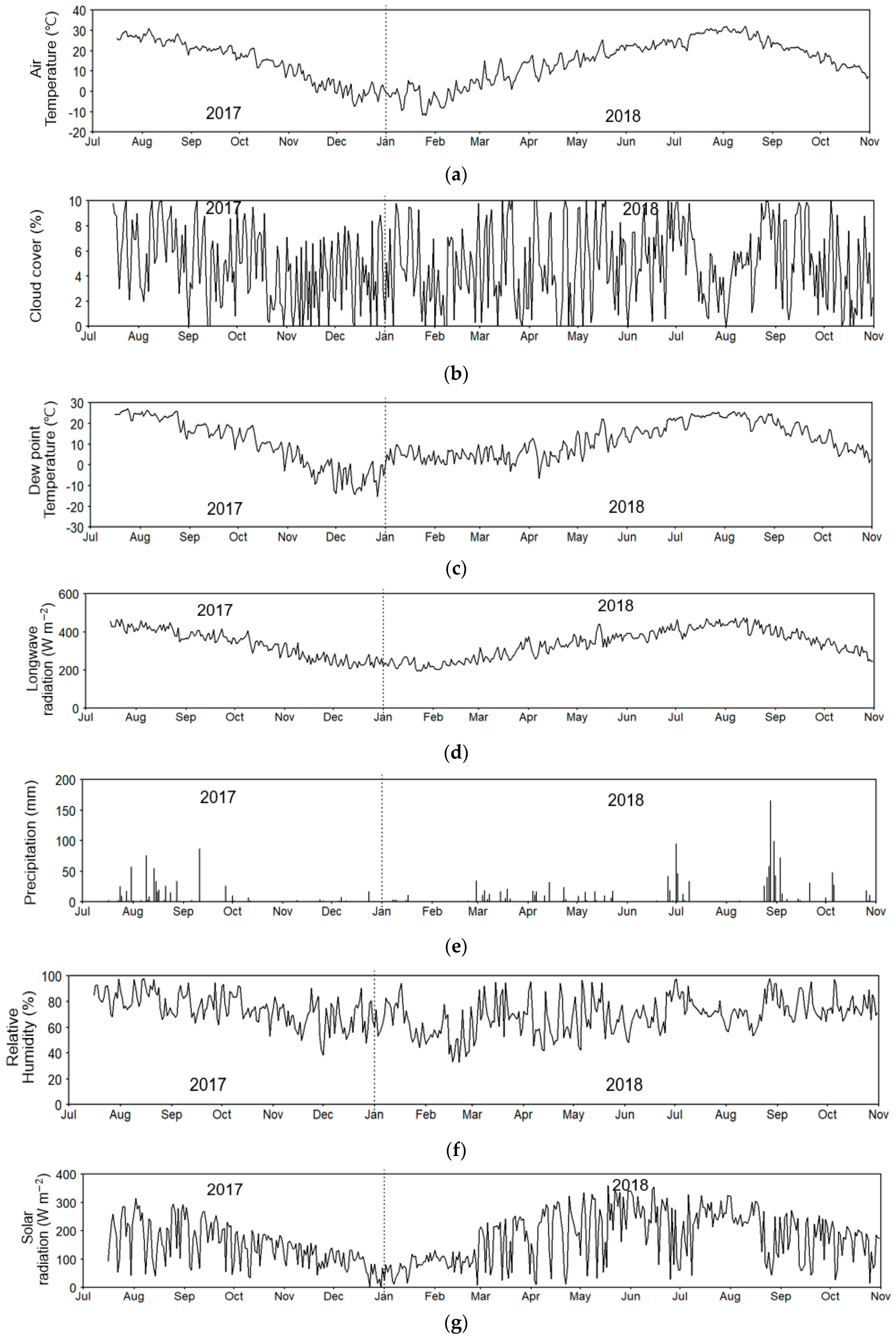
2.2. Field Monitoring and Data Collection

The data utilized in this study, as well as the data flow and the development processes of the W2, LSTM, and PGDL models, are illustrated in Figure 2. Calibration (or training) data, consisting of water temperature measurements for various water depths in the reservoir, were essential for all models. The calibration data encompassed water temperature measurements obtained from the monitoring station located in front of the Daecheong Dam (Figure 1). For this purpose, the HoBO Water Temp Pro (Onset Computer Corporation, Bourne, MA, USA), a water thermometer sensor, was employed. A thermistor chain was installed at intervals of 1–3 m in the water column, and measurements were recorded every 10 min between July 2017 and August 2018.

The PB model, W2, required flow rate, inflow water temperature, and meteorological data as boundary condition forcing data [1,42]. Details on the collection of forcing data for the W2 model and the estimation of the inflow water temperature using the multiple regression equation are described in Section 2.3. The LSTM and PGDL models needed only meteorological data as input for training and testing. Meteorological data were collected from the Daejeon meteorological observatory and the Cheongnamdae automated weather station (AWS) located near the study area (Figure 1). Temperature (°C), dew point temperature (°C), precipitation (mm), relative humidity (%), solar radiation (MJ m⁻²), and wind speed (m s⁻¹) were collected from the Korea Meteorological Administration [50].

2.3. Process-Based Model (CE-QUAL-W2 (W2))

The W2 model is a two-dimensional hydrodynamic and water-quality model that can simulate water temperature, velocity fields, water-level fluctuations, and associated water-quality variation in both vertical and horizontal directions. As the W2 model assumes complete mixing in the lateral direction, it has been widely used for simulating narrow- and deep-water bodies such as the Daecheong Reservoir [51].

For modeling the Daecheong Reservoir, the numerical grid was constructed based on the digital topographic data collected in 2018 and reservoir bathymetry data surveyed in 2006 by Korea Water Resources Corporation (K-Water). The spatial range of the numerical grid was composed of six branches from the Gadeok Bridge to the Daecheong Dam, considering the shape of the reservoir (Figure 1 and Figure A1). The numerical grid comprised 165 segments in the longitudinal direction (Δx = 0.2–1.9 km) and 69 layers in the vertical direction (Δz = 0.5–2.0 m) for efficient and accurate calculations simultaneously. The reliability of the model numerical grid was evaluated by comparing the modeled water level-reservoir capacity curve with the measured one [52]. The simulation period was 24 months, from January 2017 to December 2018. For initial modeling conditions, the dam operation data provided by K-water information portal [53] was water temperature by depth.

As the boundary conditions of the model, wind direction (radian), wind speed (m s⁻¹), air temperature (°C), dew point temperature (°C), and cloud cover (%) were used to calculate the heat exchange flux between the air and water surfaces. The daily flow data collected from K-water information portal [53] and the National Water Resources Management Information System [52] were used for defining the flow boundary conditions for each inflow river and outflow structure. The water temperature of the inflow river ($T_{in}$) was calculated using the multiple regression equation (Equation (1)) developed by Chung and Oh [54].

$$T_{in}=-0.0021\mathrm{Q}+0.88285T_{air}+0.1479T_{dew}+1.3109r^2=0.822,$$

(1)

where $T_{air}$ is the air temperature (°C); $T_{dew}$ is the dew point temperature (°C); and $\mathrm{Q}$ is the flow rate (m³ s⁻¹).

2.4. Deep Learning Model (Long Short-Term Memory (LSTM))

The LSTM used in the development of PGDL is an algorithm that solves the long-term dependency problem of existing RNNs, where the predictive power of learning results decreases as the input sequence becomes longer. Consecutively, RNN has been developed to address the limitations of feedforward neural network models in sequential data prediction [55]. In the RNN algorithm, the output value of the current state ($h_t$) is expressed as a function of the previous state ($h_{t-1}$) and the current input value ($x_t$) (Equation (2)). The neural network structure in which the state is preserved over time is called a memory cell, and when the result is calculated through the activation function in the hidden state, it is transferred to the next time through the memory cell and used as an input value for recursive activity.

$$h_t=tanh\left(W_h{h}_{t-1}+W_x{x}_t\right)+b_h,$$

(2)

where $h_t$ is the hidden layer output of the current state; $tanh$ is the activation function; $W_x$ is the weight for input $x_t$; $W_h$ is the weight for hidden layer output of the previous state ($h_{t-1})$; and $b_h$ is the bias term.

LSTM is an algorithm that changes the recurrent connection for short-term memory of the existing RNN into a forget gate ($f_t)$, input gate ($i_t)$, and output gate ($o_t)$ to store the past memory, which controls the amount of memory to be sent to the next cell. In addition to the hidden vector $h_t$, LSTM has a memory cell called $c_t$ that serves as a short-term memory store for the RNN model. $c_t$ contains all necessary information from the past to the present that serves long-term memory. Unlike $h_t$, data is exchanged only within the LSTM cell and is not output outside the LSTM cell. Each gate function and memory cell function of the LSTM are described in Equations (3)–(8).

$${\tilde{c}}_t=tanh\left(W_{hc}{h}_{t-1}+W_{xc}{x}_t\right)+b_c,$$

(3)

$$f_t=\sigma \left(W_{hf}{h}_{t-1}+W_{xf}{x}_t\right)+b_f,$$

(4)

$$i_t=\sigma \left(W_{hi}{h}_{t-1}+W_{xi}{x}_t\right)+b_i,$$

(5)

$$o_t=\sigma \left(W_{ho}{h}_{t-1}+W_{xo}{x}_t\right)+b_o,$$

(6)

$$c_t=f_t\times c_{t-1}+i_t\times {\tilde{c}}_t,$$

(7)

$$h_t=o_t\times {tanh(c}_t),$$

(8)

where $x_t$ is input data; $h_{t-1}$ is the hidden layer output of the previous state; $\sigma$ and $tanh$ are activation functions; ${\tilde{c}}_t$ is candidate values; $W_{xi}$, $W_{xf}$, $W_{xo},\mathrm{a}\mathrm{n}\mathrm{d}{W}_{xc}$ are the weights of each gate and candidate values for input $x_t$; $W_{hi}$, $W_{hf}$, $W_{ho},{\mathrm{a}\mathrm{n}\mathrm{d}W}_{hc}$ are the weights of each gate and candidate values for previous state $h_{t-1}$; and $b_i$, $b_c,b_f,\mathrm{and}{b}_o$ are the bias for each gate and candidate values.

The LSTM water temperature model was developed using measured data and prediction values (${\widehat{y}}_{d,t}:d\in \left[1,N_d\right],t\in \left[1,T\right]$) for each water depth (d) and time (t) (Equation (9)). For the error of the LSTM model, the root mean square error (RMSE) was obtained from the square of the deviation between the simulated and measured values, considering the available number $S=\left\{\left(d,t\right):y_{d,t}\right\}$ of the measured value (Equation (10)).

$${\widehat{y}}_{d,t}=W_y{h}_t,$$

(9)

$${\mathcal{L}}_{LSTM}=\sqrt{\frac{1}{S}{\sum }_{(d,t)\in S}{(y_{d,t}-{\widehat{y}}_{d,t})}^2}.$$

(10)

In this study, the LSTM model was constructed using the TensorFlow-Keras library of Python 3.10.6. From a total of 399 datasets measured between July 2017 and October 2018, the data from July 2017 to July 2018 (279 datasets) were used as a training dataset, and the data from July 2018 to October 2018 (120 datasets) were used as a testing dataset.

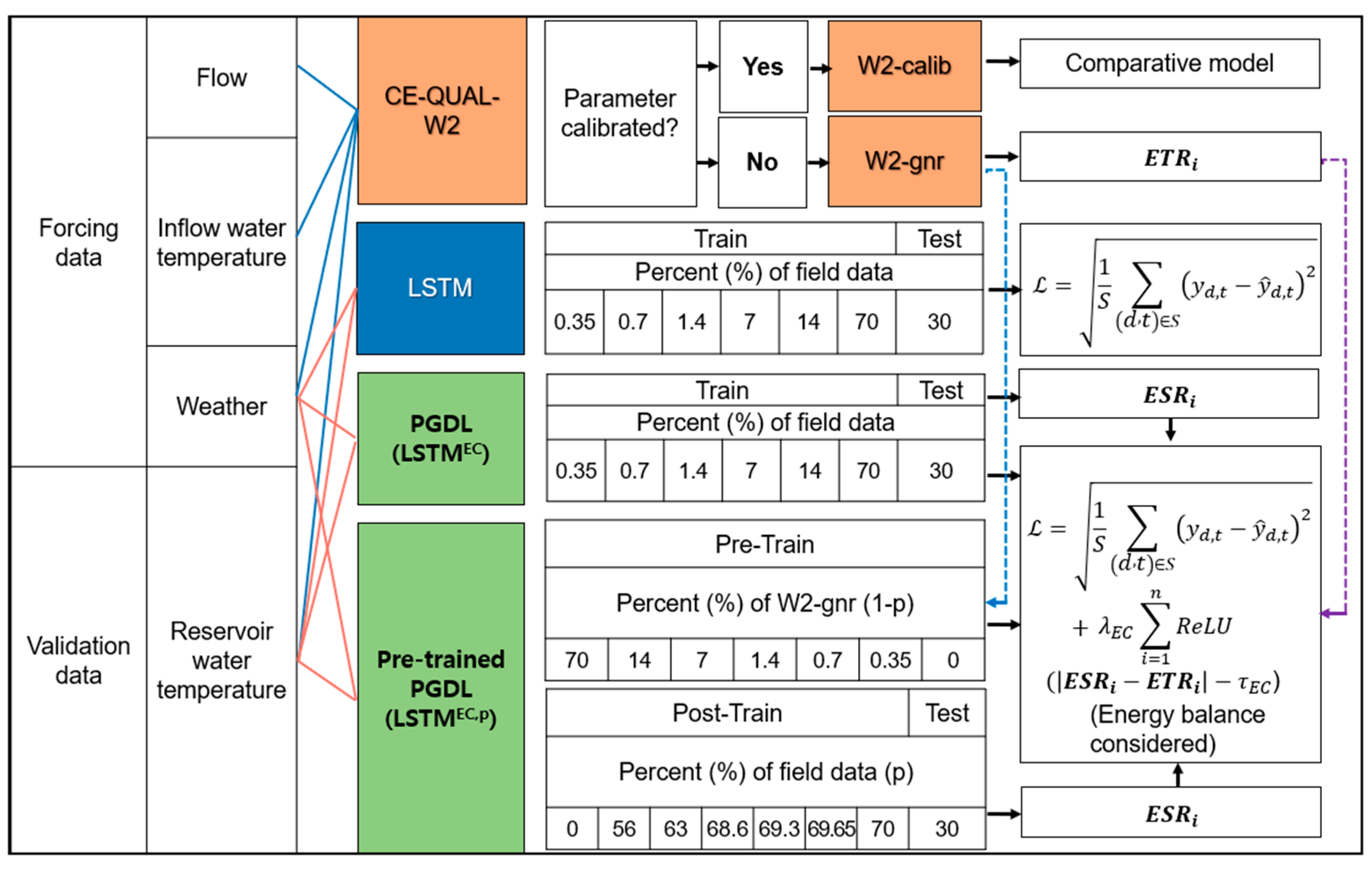
2.5. Development of the PGDL Model

Figure 2 illustrates the construction and development process of the PGDL models, including the pre-trained PGDL model, where the LSTM model is combined with the W2 model. The training data for the PGDL model consisted of the same meteorological data (relative humidity, dew point temperature, air temperature, precipitation, wind speed, short-wave radiation, and long-wave radiation) used in the W2 model for water temperature prediction, including the measured water temperature for each water depth in the reservoir. The water temperature data used for training and testing the PGDL model were identical to the data used for the LSTM model. The summary of input data for the PGDL model and the time series trend are presented in

Table A1. Summary of input data used for PGDL model development.

Variables	Unit	Value
Sample size	n	399
Air temperature	°C	17.5 ($\pm$8.9) *
Cloud cover	%	5.0 ($\pm 3$.0)
Dew point temperature	°C	12.6 ($\pm$9.8)
Long-wave radiation	W m−2	356.1 ($\pm$64.8)
Precipitation	mm	4.4 ($\pm$15.2)
Relative humidity	%	73.0 ($\pm$12.2)
Solar radiation	W/m−2	168.8 ($\pm$86.8)
Wind speed	m s−1	1.3 ($\pm 0$.5)

Note: * Mean ($\pm$ standard deviation).

and Figure A2, respectively.

The PGDL model is based on the LSTM model and trained by adding a penalty in the loss function to address energy balance violations. The performance of the PGDL model in water temperature prediction was evaluated by comparing the errors with the measured values, considering different seasons and water depths, and assessing satisfaction with the energy conservation law. Comparative models used for evaluation included the uncalibrated CE-QUAL-W2 (W2-gnr), calibrated W2 (W2-calib), LSTM without energy conservation consideration, a PGDL model incorporating the energy conservation term in the LSTM objective function (LSTM^EC), and a pre-trained PGDL model using W2-gnr (LSTM^EC,p) (Figure 2). Additionally, LSTM, LSTM^EC, and LSTM^EC,p comprised various sub-models based on the ratio of field measurement data to the W2-gnr model results used in the training dataset. The percentage of field measurement data (p = 0.5%, 1%, 2%, 10%, 20%, and 100%) in the pre-training dataset was determined according to a previous study by Read et al. [24]. The remaining training data (i.e., 1 − p) for post-training were supplemented using W2-gnr. However, the amount of testing data remained consistent across all cases.

The parameters of the W2-gnr and W2-calib models for reservoir temperature calibration are provided in

Table A2. Parameter values used for water temperature simulations in W2-gnr and W2-calib.

Parameters	Units	Description	The Values of Model Parameters
			W2-gnr	W2-calib
AX	m2 s−1	Horizontal eddy viscosity	1.0	1.0
DX	m2 s−1	Horizontal eddy diffusivity	1.0	1.0
WSC	-	Wind sheltering coefficient	0.85	1.0–1.5
FRICT	m1/2 s−1	Chezy coefficient	70	70
EXH2O	m−1	Extinction coefficient for pure water	0.25	0.45
BETA	-	Solar radiation absorbed in the surface layer	0.45	0.45
CBHE	W m−2 s−1	Coefficient of bottom heat exchange	0.3	0.45

. The hyperparameters of the LSTM, LSTM^EC, and LSTM^EC,p models were set through the GridSearchCV and trial-and-error methods to converge to the minimum error. The final set of hyperparameters included 20 hidden units, 40,000–50,000 epochs, a batch size of 32–64, dropout rates of 0.1–0.2, a learning rate of 0.0001–0.01, one LSTM layer, three dense layers, one dropout layer, and the Adam optimization algorithm (

Table A3. Hyperparameters of LSTM, LSTM^EC, and LSTM^EC,p used for reservoir water temperature prediction.

Model	Hyperparameters	Definition	Hyperparameter Range	Defined Hyperparameters
LSTM	Learning rate	Amount of change in weight that is updated during learning.	[0.0001, 0.1]	[0.0001, 0.01]
	Batch size	Group size to divide training data into several groups.	[32, 64]	[32, 64]
	Epochs	Number of learning iterations.	[1000, 50,000]	[40,000, 50,000]
	Optimizer	Optimization algorithm used for training.	[SGD, RMSprop, Adam]	Adam
	Dropout rate	Dropout setting applied to layers.	[0, 1]	[0.1, 0.2]
LSTMEC	Learning rate	Amount of change in weight that is updated during learning.	[0.0001, 0.1]	[0.0001, 0.01]
	Batch size	Group size to divide training data into several groups.	[32, 64]	[32, 64]
	Epochs	Number of learning iterations.	[1000, 50,000]	[40,000, 50,000]
	Optimizer	Optimization algorithm used for training.	[SGD, RMSprop, Adam]	Adam
	Dropout rate	Dropout setting applied to layers.	[0, 1]	[0.1, 0.2]
LSTMEC,p	Learning rate	Amount of change in weight that is updated during learning.	[0.0001, 0.1]	[0.0001, 0.01]
	Batch size	Group size to divide training data into several groups.	[32, 64]	[32, 64]
	Epochs	Number of learning iterations.	[1000, 50,000]	[40,000, 50,000]
	Optimizer	Optimization algorithm used for training.	[SGD, RMSprop, Adam]	Adam
	Dropout rate	Dropout setting applied to layers.	[0, 1]	[0.1, 0.2]

).

2.6. Validation of Energy Conservation in the PGDL Model

Conservation of energy is a fundamental principle that plays a crucial role in water temperature predictions within PBMs. It holds significant importance in evaluating the physical validity of predicted outcomes. The conservation of thermal energy within a waterbody is essential for accurate temperature predictions, as the thermal energy flux through the waterbody’s boundaries affects its temperature [24]. When the inflow heat flux exceeds the outflow heat flux, the waterbody’s temperature increases, and vice versa.

The validation of energy conservation within the PGDL model was performed by examining the energy exchanged through the reservoir boundary (${ETR}_t)$ and the energy change resulting from spatial temperature variations within the reservoir (${ESR}_t$) during the computational period. Essentially, the total heat energy within the Daecheong Reservoir at a specific time t (${ESR}_t$) was calculated as the summation of the total heat energy from the previous time (${ESR}_{t-1}$) and the summation of heat energy contributions from each water layer, estimated using the water temperature ($T_{d,t}$) predicted by the LSTM model (as expressed in Equation (11)).

$${ESR}_t={ESR}_{t-1}+C_w\sum {\rho }_{d,t}{T}_{d,t}{V}_{d,t},$$

(11)

where $C_w$ is the specific heat capacity of water (4186 J kg⁻¹ °C⁻¹); ${\rho }_{d,t}$, $T_{d,t}$, and $V_{d,t}$ correspond to the density (kg m⁻³), water temperature (°C), and water volume (m³), respectively, at time t and depth d.

The value of ${ETR}_t$ was obtained by summing the heat fluxes entering and exiting through different boundaries, as described in Equation (12). In this study, the heat fluxes considered for calculating ${ETR}_t$included evaporation-induced heat outflow (TSSEV), heat inflow due to rainfall (TSSPR), heat inflow at the upstream boundary condition (TSSUH), heat outflow at the downstream boundary condition (TSSDH), heat exchange at the water surface (TSSS), and heat exchange at the bottom of the water body (TSSB). Other factors were not considered, assuming their impact was negligible. The heat exchange between the atmosphere and water surface involved solar short-wave radiation, water long-wave radiation, atmospheric long-wave radiation, conduction, convection, evaporation, and condensation. The calculation of ${ETR}_t$ was performed using the energy balance calculation (EBC) function provided by the W2 model.

$${ETR}_t=TSSEV+TSSPR+TSSDT+TSSUH+TSSDH+TSSS+TSSB+TSSICE,$$

(12)

where TSSEV is evaporative heat loss; TSSPR is rainfall heat inflow; TSSDT is nonpoint source heat inflow; TSSUH is heat inflow at the upstream boundary; TSSDH is heat effluent at the downstream boundary; TSSS is heat exchange at the water surface; TSSB is heat exchange at the bottom of the waterbody; and TSSICE refers to heat exchange by freezing.

To train the LSTM^EC model to follow the principles of the physical laws, an algorithm was employed that incorporated a penalty into the cost function (also known as the objective function) whenever the energy conservation law was violated [26]. The total training error ($\mathcal{L}$) comprised two components: the error of the LSTM model (${\mathcal{L}}_{LSTM})$ and the error arising from the violation of the energy conservation law (${\mathcal{L}}_{EC})$(as depicted in Equation (13)). The performance of ${\mathcal{L}}_{LSTM}$was evaluated by quantifying the difference between the measured and predicted values (as shown in Equation (10)). To address the violation of the energy conservation law, ${\mathcal{L}}_{EC}$ introduced a rectified linear unit (ReLU) activation function, which was integrated into the error function as a penalty when the disparity between ${ETR}_t$ and ${ESR}_t$ exceeded a certain threshold (${\tau }_{EC}$) (as expressed in Equation (14)). A coefficient ${\lambda }_{EC}$ was employed to adjust the weight of ${\mathcal{L}}_{EC}$ within the total training error and was set to 0.01 based on a previous study by Read et al. [24]. Smaller values of ${\lambda }_{EC}$ may compromise the satisfaction of energy conservation but can reduce training loss, while excessively large values of ${\lambda }_{EC}$ can force the LSTM model to strictly follow the physical relationship, potentially leading to suboptimal performance.

$$\mathcal{L}={\mathcal{L}}_{LSTM}+{\lambda }_{EC}{\mathcal{L}}_{EC},$$

(13)

$${\mathcal{L}}_{EC}={\sum }_{i=1}^{n}ReLU(\left|{ESR}_i-{ETR}_i\right|-{\tau }_{EC}),$$

(14)

where ${\tau }_{EC}$ is a threshold value for loss of energy conservation, which was introduced to consider factors ignored in calculating the amount of heat exchange through boundary conditions and observation errors in meteorological data. For ${\tau }_{EC}$, the maximum value of the absolute difference between daily averaged spatially integrated energy (ESR) and (ETR) ($\left|{ESR}_i-{ETR}_i\right|)$ calculated in W2 that satisfies the energy balance was used [24,56].

2.7. Pre-Training of LSTM Using an Uncalibrated W2 (W2-gnr) Model

In this study, a novel approach was employed to address the challenges posed by limited, high-quality data in water environment modeling. Pre-training of the LSTM^EC,p model was conducted using the results of the W2-gnr model, which served as valuable data. Although these results were incomplete, they adhered to the energy conservation law and accurately captured the physical characteristics and meteorological conditions of the reservoir. By leveraging the mechanical principles embedded in the W2 model, the LSTM^EC,p model generated water temperature predictions that reflected these principles [56]. Specifically, the spatiotemporal predictions of water temperature over time and depth from the W2 model were utilized as training data for the LSTM^EC,p model. Through fine-tuning, the LSTM^EC,p model’s parameters were adjusted across all layers of the LSTM model using available measured data, enabling the evaluation of its performance in predicting water temperature with limited measured data. This approach effectively combined the strengths of the pre-trained LSTM^EC,p model and the available measured data to enhance prediction accuracy and overcome data limitations.

2.8. Evaluation of Model Performance

The evaluation of reservoir water temperature prediction performance involved assessing the satisfaction of the energy conservation law (ETR = ESR) and utilizing error indices to compare the measured and predicted values. The error indices employed for model evaluation included the absolute mean error (AME), RMSE, and Nash–Sutcliffe efficiency (NSE). These error indices provided quantitative measures to assess the accuracy and reliability of the water temperature predictions.

3. Results

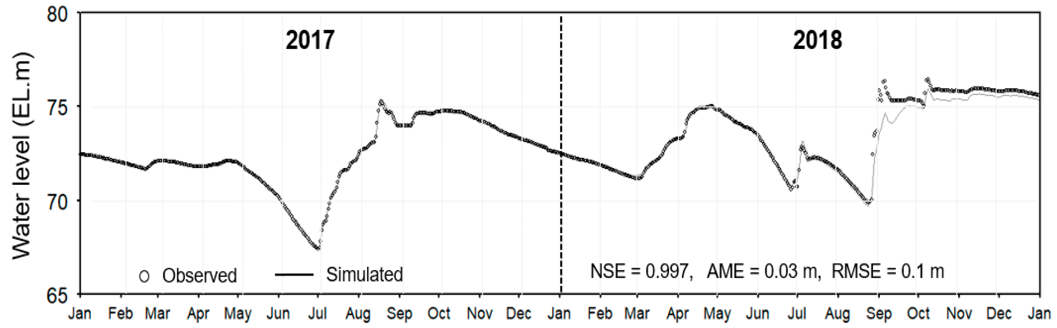
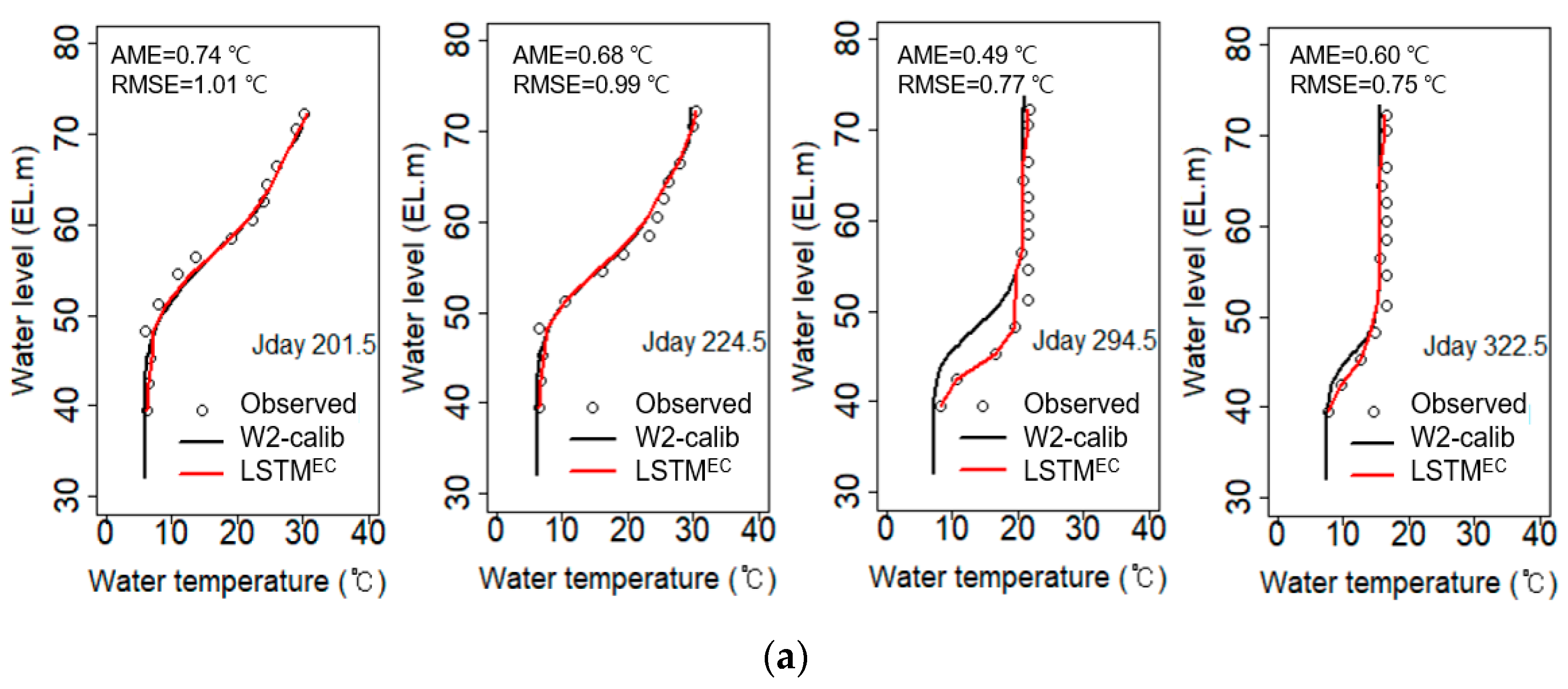
3.1. Validation of the CE-QUAL-W2 Model

The W2 model employed in this study has a well-established history of being applied to water temperature prediction in the Daecheong Reservoir, and it has undergone sufficient calibration in previous studies [54,57,58]. Consequently, there was no need for additional calibration in this study. Instead, the performance of the W2 model in predicting water level and temperature during the simulation period was validated by quantifying the error between the predicted and measured values. For the PGDL and pre-trained PGDL models, the W2-gnr model provided the necessary data (ETR and pre-training data), eliminating the need for separate model calibration. Hence, the results of the W2-calib model were exclusively used for the purpose of comparing the performance of different models (Figure 2).

Figure 3 compares the measured and simulated water levels during the 2 year simulation period from 2017 to 2018. As a result of the comparative analysis, the W2 model properly reproduced the measured changes in the water level according to the temporal fluctuations of the inflow and discharge in the Daecheong Reservoir and showed high prediction reliability with AME = 0.03 m, RMSE = 0.10 m, and NSE = 0.997. The simulated water level underestimated the measured value after September 2018 because of the uncertainty involved in calculating the inflow from the unmeasured surrounding tributaries using a simple basin area ratio.

The water temperature prediction performance of the W2 model by water depth was validated by comparing the water temperature profile data measured at the monitoring station situated in front of the dam (Figure 1) and the simulation results (Figure 4). The errors between simulated water temperature (black line) and measured values (open circles) were AME = 0.45–1.31 °C, RMSE = 0.51–1.43 °C for 279 training datasets, and AME = 0.52–2.43 °C, RMSE = 0.61–2.91 °C for 120 testing datasets. The simulation results showed that the seasonal changes in the thermal stratification structure were well reflected. During the 2 year simulation period, the W2 model reproduced the hydrothermal stratification process in summer, vertical mixing in autumn and winter, and hydrothermal stratification regeneration in the following year. However, in the training data, the model failed to accurately replicate the downward movement of the thermocline on Julian Day 294.5, while in the testing data, the model overestimated the surface water temperature on Julian Day 594.5 and struggled to properly reproduce the thermocline on Julian Day 608.5. This error can be attributed to uncertainties in the input data and parameters of the process model, which made it difficult to accurately reproduce the density flow entering the middle layer during rainfall as well as the change in stratification structure caused by turbulent wind-driven mixing in the surface layer [59,60,61].

The sources and sinks of the reservoir heat energy as calculated by W2 during the simulation period were analyzed (Figure A3). As a result of heat balance analysis, the net heat flux across the water surface (H_n) of the Daecheong Reservoir was in the range of −389 to 942 (average −5.0) W m⁻². H_n exhibited a high value in summer, a period of rising water temperature, and a negative value in winter, a period of decreasing water temperature. Evaporative heat loss due to water evaporation showed the highest value in summer when temperatures rose, and heat conduction (sensible heat loss) had the highest value in winter when temperatures decreased.

3.2. Prediction Performance of the PGDL Model

Table 1. Comparison of performance of W2-gnr, W2-calib, LSTM, LSTM^EC, and LSTM^EC,p according to the percentage of field data used in the model training phase.

Model	RMSE (°C)
	Proportion of Field Data Used in the Model Training Phase (%)
	0	0.5	1	2	10	20	100
W2-gnr	-	-	-	-	-	-	1.930
W2-calib	-	-	-	-	-	-	1.781
LSTM	-	15.978 $(\pm$0.380)	9.403 $(\pm$0.284)	2.432 $(\pm$0.257)	0.289 $(\pm$0.113)	0.131 $(\pm$0.089)	0.062 $(\pm$0.010)
LSTMEC	-	15.007 $(\pm$0.319)	8.915 $(\pm$0.256)	2.229 $(\pm$0.212)	0.243 $(\pm$0.100)	0.092 $(\pm$0.033)	0.042 $(\pm$0.007)
LSTMEC,p	7.214 $(\pm$0.327)	3.007 $(\pm$0.301)	2.015 $(\pm$0.156)	1.160 $(\pm$0.115)	0.230 $(\pm$0.088)	0.078 $(\pm$0.012)	0.018 $(\pm$0.001)

Note: W2-gnr: uncalibrated CE-QUAL-W2 model; W2-calib: calibrated CE-QUAL-W2 model; LSTM: long short-term memory (LSTM) model trained with field data without considering energy conservation; LSTMEC: LSTM model trained with field data with considering energy conservation; and LSTM^EC,p: pre-trained LSTM^EC model with W2-gnr results and then gets fine-tuned using the field data; RMSE: root mean square error.

shows the RMSE values of the W2-gnr and W2-calib models, LSTM, process-guided LSTM (LSTM^EC), and pre-trained LSTM (LSTM^EC,p). The samples were randomly selected from partial field data from the training dataset to use in training LSTM, LSTM^EC, and LSTM^EC,p; the test dataset remained unchanged. The error values presented in Table 1 correspond to the average and standard deviation of the RMSE for the results obtained by random sampling of training data. In other words, the reported results were obtained through 10-fold cross-validation, and the numbers within parentheses represent the standard deviation of the results from the 10 simulation runs.

The predictive performance of LSTM, LSTM^EC, and LSTM^EC,p models all improved as the proportion of field data increased. When the ratio of field data was 100%, LSTM^EC’s RMSE was 0.042 (±0.007) °C, showing 42.4 times and 1.5 times better prediction performance than W2-calib and LSTM, respectively. The predictive performance of W2-calib was superior to that of LSTM^EC and LSTM developed using less than 2% of the total field data for training, but LSTM^EC and LSTM showed better predictive performance than W2-calib when the field data ratio was ≥10%. In particular, LSTM^EC showed better predictive performance than LSTM in all cases of the field data ratio (0.5% to 100%), and as the ratio increased, the difference in RMSE between LSTM and LSTM^EC narrowed. These results are consistent with the results of Read et al. [24].

To evaluate the water temperature prediction accuracy of LSTM^EC by water depth, the simulated water temperatures using the LSTM^EC (red line) and W2-calib model (black line) were compared with the measured water temperatures (open circles) in Figure 4. LSTM^EC appropriately simulated the change in water temperature profile by water depth over time in both the training and testing phases. LSTM^EC showed high prediction accuracy with error values of AME = 0.14–1.64 °C and RMSE = 0.16–1.87 °C, which corresponds to better prediction performance than the W2-calib model (AME = 0.45–2.43 °C, RMSE = 0.51–2.91 °C). In particular, when examining the substantial errors observed in the water temperature predictions near the thermocline zone as simulated by the W2 model, the LSTM^EC model exhibited markedly improved outcomes.

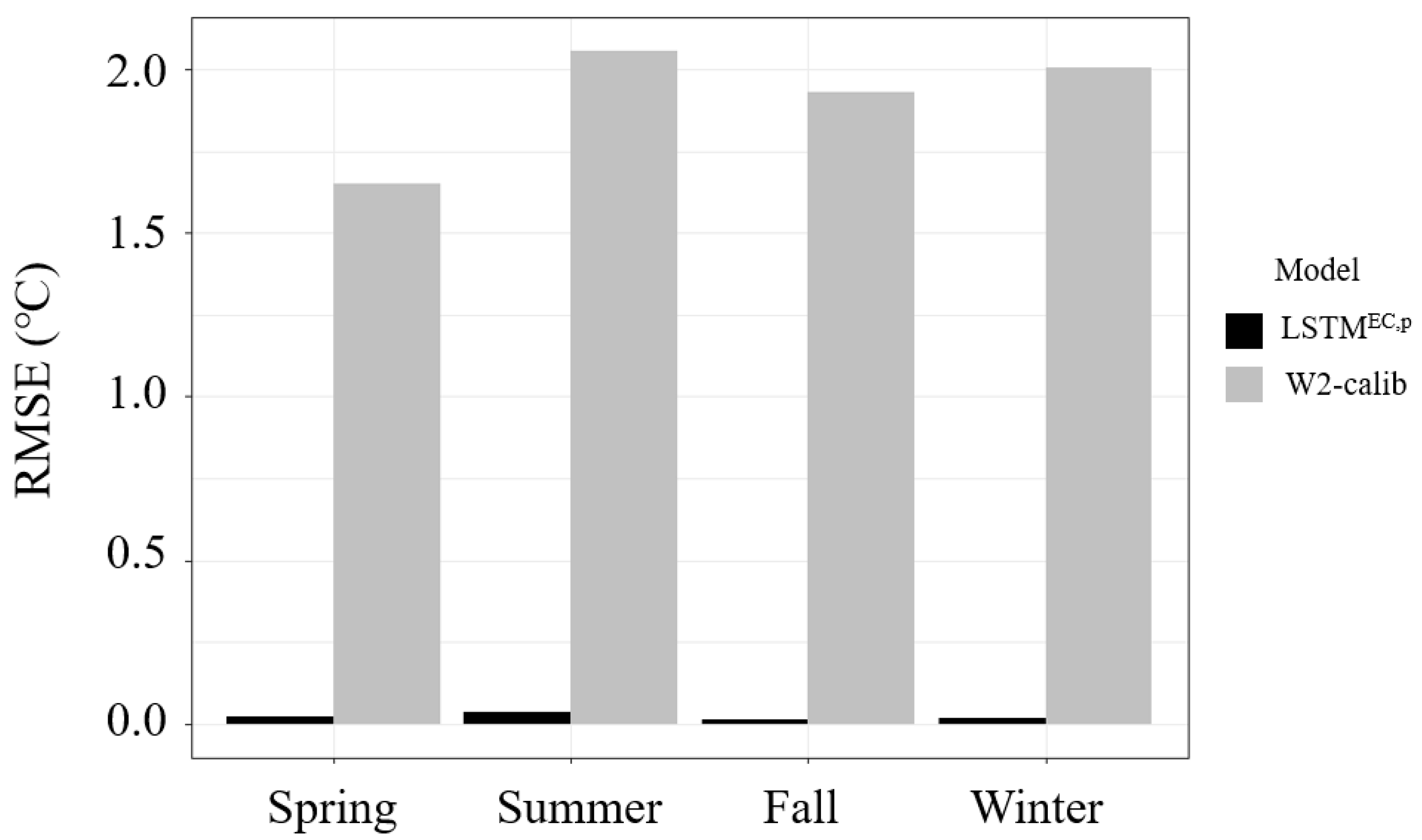
3.3. Prediction Performance of the Pre-Trained PGDL Model

To overcome the problem of deteriorating prediction performance of the LSTM^EC model due to the lack of training data, which is the major drawback of the deep learning (DL) model, a pre-training technique that can improve model prediction accuracy with a small amount of measured data was used, and the error for each model was compared according to the ratio of the measured data (Table 1). In the pre-training method, the neural network of the LSTM^EC model was trained using the results of the W2-gnr model as training data. The hydraulic model parameters that affect water temperature prediction results in the W2 model include longitudinal eddy viscosity (AX), longitudinal eddy diffusivity (DX), Chezy coefficient (FRICT), wind sheltering coefficient (WSC), solar radiation absorbed in the surface layer (BETA), and extinction coefficient for pure water (EXH2O). The W2-gnr used the default values for all these coefficients. Consequently, the RMSE of W2-gnr was approximately 1.930 °C, which was higher than that of other models (Table 1). However, as the mechanical model was simulated based on physical laws, these results were learning results considering energy conservation. Therefore, by using the results of the W2-gnr model as training data for the LSTM model, it is possible to build a deep learning model that produces results that satisfy the physical laws inherent in the physical model. The LSTM^EC,p model, which was pre-trained using 100% of the W2-gnr results, had an average RMSE of 7.214 °C, which increased by 3.74 and 4.05 times compared to W2-gnr and W2-calib, respectively. In contrast, the LSTM^EC,p model, pre-trained with 98% of the W2-gnr prediction results and post-trained using 2% of the filed data, reduced RMSE by 1.66 and 1.54 times, respectively, compared to W2-gnr and W2-calib.

The standard deviation, centered root mean square difference (CRMSE), and correlation coefficient of the measured and simulated values for each model were simultaneously compared and analyzed using a Taylor diagram (Figure 5). From the analysis, most of the LSTM^EC,p and LSTM^EC models except for LSTM^EC,p,0% were found to be very close to the measured values, and the error values were also significantly reduced. In particular, the LSTM^EC,p,10% model using only 10% of the field data showed a lower CRMSE value than the PBMs.

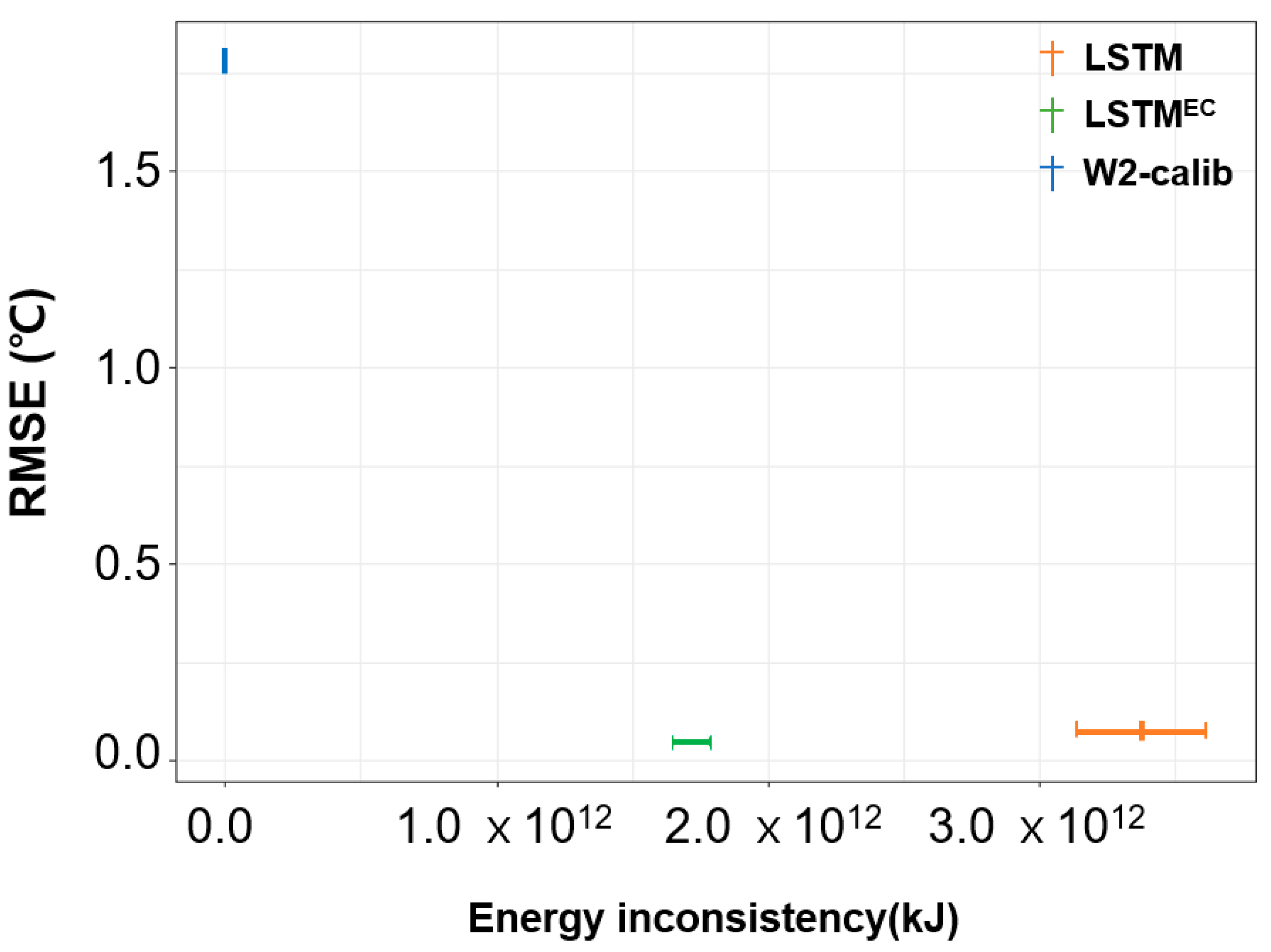
3.4. Evaluating the Energy Consistency of the PGDL Model

One of the strengths of the LSTM^EC model is that it can secure physical law consistency, which is a weakness of the LSTM model. To evaluate the satisfaction of the energy conservation law in LSTM^EC, the time series changes of ETR and ESR during the simulation period were compared along with the results of W2-calib and LSTM, as shown in Figure 6. The coincidence of ETR and ESR means that the conservation law of thermal energy changes along the reservoir boundary and inside the reservoir water body is satisfied. During the simulation period, the W2-calib model based on physical laws matched the changes in ETR and ESR very well (Figure 6a). The W2-calib model predicted reservoir water temperature by considering air-water heat exchange and heat flux at inflow and outflow interfaces. At each calculation time, the model checked the heat balance and thus satisfied the energy conservation law. However, in the case of LSTM, which is a DDM lacking physical laws, the discrepancy between ETR and ESR was confirmed in most periods, and the difference increased more in winter (Figure 6b). On the other hand, LSTM^EC with the energy conservation term added to the objective function showed lower energy agreement than the W2-calib model but better energy agreement than the LSTM model (Figure 6c). From these results, it can be confirmed that the PGDL algorithm contributes to improving the limitations of deep learning models.

The relationship between the energy inconsistency (x-axis) and RMSE (y-axis) of W2-calib, LSTM, and LSTM^EC is presented in Figure A4. The lengths of the LSTM and LSTM^EC bars in the graph cover the 10-fold cross-validation results. The W2-calib corresponds to a model developed for satisfying the energy conservation law, and therefore, it showed an energy mismatch close to zero, but its RMSE showed an average of 42.4 times and 28.7 times greater than those of LSTM^EC and LSTM, respectively. In contrast, the LSTM^EC model demonstrated improved predictive performance compared to both the W2-calib and LSTM models and exhibited a lower degree of energy mismatch than the standalone LSTM, demonstrating the potential for enhancing the physical consistency of the LSTM model.

Recently, the application of DDM techniques such as ML and deep learning has rapidly progressed in the field of water quality prediction [62,63,64]. However, owing to their lack of dependence on physical laws, these models may overlook important underlying mechanisms. The PGDL algorithm, demonstrated by the hybrid results of the W2 and LSTM models, has the potential to address these issues not only for predicting water temperature in stratified reservoirs but also for water quality prediction.

4. Discussion

4.1. Comparative Analysis of Water Temperature Prediction Errors

Figure 7 illustrates the water temperature prediction error (RMSE) at various water depths for the W2-gnr, W2-calib, LSTM, LSTM^EC, and LSTM^EC,p models. In the case of the W2 model, both the W2-gnr and W2-calib models showed similar RMSE values in the surface layer (EL. 63–75 m), but the error of the W2-calib model decreased with the increase in water depth. Overall, the LSTM, LSTM^EC, and LSTM^EC,p models exhibited lower RMSE values compared to the process-based W2-gnr and W2-calib models across all depths. When comparing LSTM^EC and LSTM^EC,p, the RMSE values of LSTM^EC,p, which was pre-trained using the simulation results of W2-gnr, were lower at all depths. These results highlight the significant impact of pre-training on reducing model error. Furthermore, the LSTM^EC,p model demonstrated lower RMSE values than the W2-gnr and W2-calib models, with the difference being particularly prominent in the metalimnion layer (between 40 and 55 m). The increased error of the PBM in the thermocline, where water temperature changes rapidly, is not solely due to numerical diffusion issues but also due to the accurate representation of complex hydrodynamic processes such as density flow, turbulent mixing, and internal waves, which are crucial for reproducing the water temperature stratification phenomenon. In particular, reservoir stratification is influenced not only by temperature-related density differences but also by light attenuation caused by suspended matter, phytoplankton, and dissolved matter, contributing to the uncertainties associated with these parameters and resulting in erroneous water temperature predictions. Thus, accurately capturing the dynamic changes in thermal stratification structures in deep reservoirs remains challenging for most PBMs, including W2 [61,65]. However, data-based deep learning models demonstrate superior performance by learning from patterns in the training data rather than relying solely on physical processes.

In the seasonal error analysis (Figure A5 and Figure A6), the water temperature prediction errors of the W2-calib model varied across different seasons and depths. Specifically, during the spring, when stratification started, the W2-calib model exhibited large errors in the surface layer. During summer and autumn, the errors were prominent in the middle and lower layers, respectively. The lowest errors were observed during the winter, when stratification was disrupted. In contrast, the LSTM^EC,p model consistently showed significantly lower RMSE values compared to the W2-calib model across all seasons and depths. This indicates that the PGDL model has the potential to address critical prediction challenges in the aquatic environment. Furthermore, the application of PGDL models can contribute to the convergence of deductive and inductive methods, theory, and experience, allowing for improved water temperature predictions [66,67,68]. These findings emphasize the effectiveness and versatility of the PGDL model in improving water temperature prediction accuracy in stratified reservoirs.

4.2. Applicability of the PGDL Model for Water Quality Modeling

The framework of the PGDL model developed in this study for water temperature prediction can be effectively extended to various water temperature and water quality modeling applications. Water temperature plays a crucial role in shaping the spatiotemporal distribution of physical, chemical, and ecological variables in aquatic ecosystems [69,70]. It strongly influences the concentration of dissolved oxygen, nutrient conversion rates, metabolic activities of aquatic organisms, phytoplankton productivity, and biochemical reactions. Notably, deviations from critical water temperature values can significantly impact fish populations, leading to increased mortality rates [71,72,73]. Additionally, accurate prediction of water temperature by depth in deep reservoirs is essential for managing selective discharge facilities and controlling downstream water temperature and quality [74,75,76]. Furthermore, PGDL models have proven to be highly effective in assessing the impacts of climate change on reservoir water temperatures and thermal stratification patterns over extended time periods, relying solely on weather data.

Surface water temperature is influenced by various factors, including flow rate, solar radiation [77], channel morphology [78], point source emissions [79], air–water heat exchange, and ice cover [80]. Therefore, predicting accurate water temperatures in space and time becomes challenging due to these complex interactions. PBMs leverage scientific principles and knowledge to predict water temperature based on physical laws that reflect water flow systems, river morphology, and heat changes in water bodies related to temperature [81,82]. However, for deep lakes and reservoirs, the model complexity increases, requiring multidimensional models that consider intricate mixing processes. This complexity introduces higher uncertainty in model structure and input data, as well as increased calibration and validation costs [4,5,6].

To date, most PGDL models in environmental studies have employed zero- or one-dimensional PBMs to predict variables such as water temperature [54] and evapotranspiration [83]. These PGDL models [24,56] have consistently outperformed standalone PBMs and DL models in water temperature prediction, exhibiting superior performance in meeting energy conservation requirements compared to the original DL models. Some studies have also used the GLM model, a dynamic PBM that accounts for vertical heat exchange in the water bodies that conform to this one-dimensional assumption [84,85,86]. In this study, the PGDL is demonstrated to be a powerful algorithm for predicting water temperature stratification in artificial dam reservoirs with complex topographical features.

Recently, limited efforts have been made to develop PGDL models capable of predicting lake water quality. Hanson et al. [44] employed the PGDL model to predict the phosphorus cycle and epilimnion phosphorus concentration in Lake Mendota, Wisconsin, USA. They demonstrated the potential of the PGDL model to enhance water quality predictions beyond just water temperature. To effectively utilize the PGDL model for water quality prediction, obtaining accurate and precise boundary condition data in time and space is essential. In many countries, hydraulic systems are frequently monitored, while water quality monitoring is conducted less frequently, typically on a weekly or monthly basis, due to cost considerations [87,88]. However, this data collection frequency is inadequate for capturing rapidly changing pollutant loads during rainfall events. High-quality, high-resolution data are crucial for reliable and accurate water quality modeling.

The most common method used to obtain high-quality, high-resolution boundary condition data is in situ monitoring. With advances in sensor technology, the use of automated online smart monitoring systems and mobile-based advanced environmental monitoring technologies is increasing and becoming more common. An alternative approach to obtaining high-frequency boundary condition data is to construct an ML model based on measured data and use the model’s predictions for boundary conditions in PBM and as training data for DDM [89]. Kim et al. [90] and Mahlathi et al. [91] are good examples of representative studies that applied DDM prediction results to PBM.

In summary, obtaining high-frequency, high-resolution boundary condition data is crucial for expanding and implementing the PGDL model for water quality modeling. Furthermore, by incorporating physical laws such as conservation of mass into the cost function of the DL model, the PGDL model can serve as an effective tool for predicting water quality in rivers and reservoirs.

4.3. Strengths of the PGDL Model in the Lack of Data

Generally, DDMs excellently discover new information and make accurate predictions with sufficient training data [92], but suffer from interpretability and generalization problems due to decreased predictive accuracy without quality data. Unfortunately, the collection of most environmental data is costly and time-consuming, and there are only a limited number of appropriate monitoring sites. Moreover, collected data are frequently inappropriate as input for DDMs because unexpected circumstances often result in erroneous or missing data [93,94].

This study applied the thermistor chain to generate high-frequency water temperature data at 10 min intervals but lacked sufficient training data for the PGDL model because of missing or suspected data points. This problem was addressed by using results from the W2-gnr model as pre-training data for the PGDL model. The PBM reflects the actual physical environment of a target water body and produces predictions based on physical laws. Therefore, if the DDM is pre-trained because the PBM was retrained with a small amount of measurement data, the limitations of the short test period and insufficient training data can be resolved [24,95]. Pre-trained with W2-gnr, LSTM^EC,p yielded better predictions than LSTM, LSTM^EC, and W2-calib when only 2% of total field data were used. Comparative evaluation of prediction performance by water depth and season further demonstrated the predictive superiority of LSTM^EC,p (Figure 6, Figure A4 and Figure A5). These results suggest that the hybrid PBM and DL models used in this study are a very economical method that improves predictions of water temperature even when field measurement data are insufficient.

Transfer learning is an increasingly popular way of overcoming the lack of training data [26,96]. These methods use results from a previously learned model to train a new one. In other words, under conditions that require a certain threshold of labeled data, data obtained from an existing, related model are transferred to the target model [97,98]. Transfer learning enables fast and accurate predictions with a small amount of data, making it a valuable technique for various environmental fields, including air quality prediction. In particular, network pre-training (using part of a pre-trained network to train another network) greatly improves DDM’s predictive performance and speed [99]. Recent research in environmental sciences has begun to calibrate mechanistic models with monitoring data as a form of network pre-training. Using calibrated output results to train DDMs has seen success in hydrological applications [100,101]. For example, a study in Denmark accurately predicted runoff in 60 watersheds using an LSTM model trained using the results of the mechanistic Danish national water resources model [101].

4.4. Limitations of the PGDL Model and Scope for Future Studies

The advantages of PGDL models are considerable, combining the strengths of PBM and DDM to improve predictive accuracy while ensuring physical consistency. Specifically, PGDL assumes that PBM can adequately capture the underlying physics of a given system and that any remaining, unknown physics can be captured by DDM. However, like any model, PGDL has its own limitations, notably in terms of data quality and quantity. If the training dataset is noisy, biased, or not representative of the underlying physics, PGDL cannot improve prediction accuracy. Additionally, PGDL requires significant computational resources and expertise for development, training, and validation. Its sensitivity to the choice of hyperparameters requires considerable trial and error for optimization. Furthermore, PGDL may not generalize well to systems that are significantly different from the training data, potentially limiting its applicability to novel problems.

Future studies should focus on addressing these limitations to enhance model performance and prediction reliability. First, the quality and quantity of training data should be improved to ensure better generalization of new problems. Second, the accuracy and reliability of PBMs should be increased to better capture a given system’s underlying physics. Third, increasing the efficacy of hyperparameter tuning will help lessen the need for trial and error and improve model accuracy and applicability. Fourth, the uncertainty associated with predictions should be quantified by incorporating uncertainty analysis. Finally, PGDL transferability to different systems and environments should be evaluated to determine its potential for broader applications and improve robustness.

5. Conclusions

In this study, a PGDL model was developed by adding a penalty term to the loss function of the LSTM model to resolve the violation of the law of conservation of energy, which is a limitation of LSTM, and the water temperature prediction performance in a stratified reservoir was compared and evaluated. Furthermore, by introducing a pre-training technique where the predicted results of the uncalibrated PBM were used as pre-training data, we provided an economical modeling method that can secure water temperature prediction performance even with limited field measurement data. LSTM^EC, a deep learning model trained to satisfy the law of conservation of energy, reproduced the principle of conservation of thermal energy for the W2 model based on the physical law to a certain extent and showed improved prediction performance compared to LSTM. The LSTM^EC,p model developed using the pre-training technique showed better predictive performance than the PBMs (W2-gnr and W2-calib) and DDMs (LSTM and LSTM^EC) even when limited field data were used for training.

The success of the PBM and DDM hybrid model verified the applicability of a new technique that combines the advantages of multidimensional mathematical models and data-based deep learning models. Furthermore, it was confirmed that if a PBM is used for pre-training a deep learning model, it is possible to develop a deep learning model capable of rapidly and accurately predicting water temperature based on physical laws even when the training data are insufficient. As the LSTM^EC model developed in this study can quickly and accurately predict reservoir water temperature using only meteorological data, it can be effectively applied to predict reservoir water temperature and thermal structural changes according to future climate scenarios.

In the future, PGDL accuracy, reliability, and generalizability can be improved, which will enhance the effectiveness of environmental modeling and decision-making. Continuous research is also needed to develop PGDL into a model capable of comprehensive water-quality predictions that include organic matter and nutrients.

References

1. Cole, T.M.; Buchak, E.M. CE-QUAL-W2: A Two-Dimensional, Laterally Averaged, Hydrodynamic and Water Quality Model, Version 2.0 User Manual; US Army Corps of Engineers: Washington, DC, USA, 1995; pp. 1–357. [Google Scholar]
2. Hamrick, J.M. A Three-Dimensional Environmental Fluid Dynamics Computer Code: Theoretical and Computational Aspects; Virginia Institute of Marine Science, William and Mary University: Williamsburg, VA, USA, 1992; pp. 1–317. [Google Scholar]
3. Hodges, B.; Dallimore, C. Aquatic Ecosystem Model: AEM3D v1.0 User Manual; HydroNumerics: Victoria, Australia, 2019; pp. 1–167. [Google Scholar]
4. Bouchard, D.; Knightes, C.; Chang, X.; Avant, B. Simulating multiwalled carbon nanotube transport in surface water systems using the water quality analysis simulation program (WASP). Environ. Sci. Technol. 2017, 51, 11174–11184. [Google Scholar] [CrossRef] [PubMed]
5. Arhonditsis, G.B.; Neumann, A.; Shimoda, Y.; Kim, D.K.; Dong, F.; Onandia, G.; Yang, C.; Javed, A.; Brady, M.; Visha, A.; et al. Castles built on sand or predictive limnology in action? Part A: Evaluation of an integrated modelling framework to guide adaptive management implementation in Lake Erie. Ecol. Inform. 2019, 53, 100968. [Google Scholar] [CrossRef]
6. Schuwirth, N.; Borgwardt, F.; Domisch, S.; Friedrichs, M.; Kattwinkel, M.; Kneis, D.; Kuemmerlen, M.; Langhans, S.D.; Martínez-López, J.; Vermeiren, P. How to make ecological models useful for environmental management. Ecol. Modell. 2019, 411, 108784. [Google Scholar] [CrossRef]
7. Liu, X.; Lu, D.; Zhang, A.; Liu, Q.; Jiang, G. Data-driven machine learning in environmental pollution: Gains and problems. Environ. Sci. Technol. 2022, 56, 2124–2133. [Google Scholar] [CrossRef] [PubMed]
8. Zhang, Q.; Wang, R.; Qi, Y.; Wen, F. A watershed water quality prediction model based on attention mechanism and bi-LSTM. Environ. Sci. Pollut. Res. Int. 2022, 3, 75664–75680. [Google Scholar] [CrossRef]
9. Solomatine, D.P.; Ostfeld, A. Data-driven modelling: Some past experiences and new approaches. J. Hydroinform. 2008, 10, 3–22. [Google Scholar] [CrossRef]
10. Kesavaraj, G.; Sukumaran, S. A study on classification techniques in data mining. In Proceedings of the 2013 Fourth International Conference on Computing, Communications and Networking Technologies (ICCCNT), Tiruchengode, India, 4–6 July 2013; IEEE: New York, NY, USA, 2003; pp. 1–7. [Google Scholar] [CrossRef]
11. Ghavidel, S.Z.Z.; Montaseri, M. Application of different data-driven methods for the prediction of total dissolved solids in the Zarinehroud basin. Stoch. Environ. Res. Risk Assess. 2014, 28, 2101–2118. [Google Scholar] [CrossRef]
12. Sanikhani, H.; Kisi, O.; Kiafar, H.; Ghavidel, S.Z.Z. Comparison of different data-driven approaches for modeling Lake Level fluctuations: The case of Manyas and Tuz Lakes (Turkey). Water Resour. Manag. 2015, 29, 1557–1574. [Google Scholar] [CrossRef]
13. Amaranto, A.; Mazzoleni, M. B-AMA: A python-coded protocol to enhance the application of data-driven models in hydrology. Environ. Modell. Softw. 2023, 160, 105609. [Google Scholar] [CrossRef]
14. Granata, F.; Nunno, F.D. Neuroforecasting of daily streamflows in the UK for short- and medium-term horizons: A novel insight. J. Hydrol. 2023, 624, 129888. [Google Scholar] [CrossRef]
15. Nunno, F.D.; Zhu, S.; Ptak, M.; Sojka, M.; Granata, F. A stacked machine learning model for multi-step ahead prediction of lake surface water temperature. Sci. Total Environ. 2023, 890, 164323. [Google Scholar] [CrossRef] [PubMed]
16. Cha, Y.K.; Shin, J.H.; Kim, Y.W. Data-driven modeling of freshwater aquatic systems: Status and prospects. J. Korean Soc. Water Environ. 2020, 36, 611–620. [Google Scholar] [CrossRef]
17. Liu, Z.; Cheng, L.; Lin, K.; Cai, H. A hybrid bayesian vine model for water level prediction. Environ. Modell. Softw. 2021, 142, 105075. [Google Scholar] [CrossRef]
18. Majeske, N.; Zhang, X.; Sabaj, M.; Gong, L.; Zhu, C.; Azad, A. Inductive predictions of hydrologic events using a Long Short-Term memory network and the Soil and water Assessment Tool. Environ. Modell. Softw. 2022, 152, 105400. [Google Scholar] [CrossRef]
19. LeCun, Y.; Bengio, Y.; Hinton, G. Deep learning. Nature 2015, 521, 436–444. [Google Scholar] [CrossRef]
20. Hutchinson, L.; Steiert, B.; Soubret, A.; Wagg, J.; Phipps, A.; Peck, R.; Charoin, J.E.; Ribba, B. Models and machines: How deep learning will take clinical pharmacology to the next level. CPT Pharmacomet. Syst. Pharmacol. 2019, 8, 131–134. [Google Scholar] [CrossRef]
21. Kratzert, F.; Klotz, D.; Herrnegger, M.; Sampson, A.K.; Hochreiter, S.; Nearing, G.S. Toward improved predictions in ungauged basins: Exploiting the power of machine learning. Water Resour. Res. 2019, 55, 11344–11354. [Google Scholar] [CrossRef]
22. Mavrovouniotis, M.L.; Chang, S. Hierarchical neural networks. Comput. Chem. Eng. 1992, 16, 347–369. [Google Scholar] [CrossRef]
23. Antonetti, M.; Zappa, M. How can expert knowledge increase the realism of conceptual hydrological models? A case study based on the concept of dominant runoff process in the Swiss Pre-Alps. Hydrol. Earth Syst. Sci. 2018, 22, 4425–4447. [Google Scholar] [CrossRef]
24. Read, J.S.; Jia, X.; Willard, J.; Appling, A.P.; Zwart, J.A.; Oliver, S.K.; Karpatne, A.; Hansen, G.J.A.; Hanson, P.C.; Watkins, W.; et al. Process-guided deep learning predictions of Lake water temperature. Water Resour. Res. 2019, 55, 9173–9190. [Google Scholar] [CrossRef]
25. Reichstein, M.; Camps-Valls, G.; Stevens, B.; Jung, M.; Denzler, J.; Carvalhais, N.; Prabhat, P. Deep learning and process understanding for data-driven earth system science. Nature 2019, 566, 195–204. [Google Scholar] [CrossRef] [PubMed]
26. Karpatne, A.; Atluri, G.; Faghmous, J.H.; Steinbach, M.; Banerjee, A.; Ganguly, A.; Shekhar, S.; Samatova, N.; Kumar, V. Theory-guided data science: A new paradigm for scientific discovery from data. IEEE Trans. Knowl. Data Eng. 2017, 29, 2318–2331. [Google Scholar] [CrossRef]
27. Vapnik, V.N. An overview of statistical learning theory. IEEE Trans. Neural Netw. 1999, 10, 988–999. [Google Scholar] [CrossRef] [PubMed]
28. Franklin, J. The elements of statistical learning: Data mining, inference and prediction. Math. Intell. 2005, 27, 83–85. [Google Scholar] [CrossRef]
29. Wong, K.C.L.; Wang, L.; Shi, P. Active model with orthotropic hyperelastic material for cardiac image analysis. Lect. Notes Comput. Sci. 2009, 5528, 229–238. [Google Scholar] [CrossRef]
30. Xu, J.; Sapp, J.L.; Dehaghani, A.R.; Gao, F.; Horacek, M.; Wang, L. Robust transmural electrophysiological imaging: Integrating sparse and dynamic physiological models into ECG-based inference. Med. Image Comput. Comput. Assist. Interv. 2015, 9350, 519–527. [Google Scholar] [CrossRef]
31. Khandelwal, A.; Karpatne, A.; Marlier, M.E.; Kim, J.Y.; Lettenmaier, D.P.; Kumar, V. An approach for global monitoring of surface water extent variations in reservoirs using MODIS data. Remote Sens. Environ. 2017, 202, 113–128. [Google Scholar] [CrossRef]
32. Khandelwal, A.; Mithal, V.; Kumar, V. Post classification label refinement using implicit ordering constraint among data instances. In Proceedings of the IEEE International Conference Data Mining, Atlantic City, NJ, USA, 14–17 November 2015; pp. 799–804. [Google Scholar] [CrossRef]
33. Kawale, J.; Liess, S.; Kumar, A.; Steinbach, M.; Snyder, P.; Kumar, V.; Ganguly, A.R.; Samatova, N.F.; Semazzi, F. A graph-based approach to find teleconnections in climate data. Stat. Analy. Data Min. 2013, 6, 158–179. [Google Scholar] [CrossRef]
34. Li, L.; Snyder, J.C.; Pelaschier, I.M.; Huang, J.; Niranjan, U.N.; Duncan, P.; Rupp, M.; Müller, K.R.; Burke, K. Understanding machine-learned density functionals. Int. J. Quantum Chem. 2016, 116, 819–833. [Google Scholar] [CrossRef]
35. Faghmous, J.H.; Frenger, I.; Yao, Y.; Warmka, R.; Lindell, A.; Kumar, V. A daily global mesoscale ocean eddy dataset from satellite altimetry. Sci. Data 2015, 2, 150028. [Google Scholar] [CrossRef]
36. Zhang, Z.; Sun, C. Structural damage identification via physics-guided machine learning: A methodology integrating pattern recognition with finite element model updating. Struct. Health Monit. 2021, 20, 1675–1688. [Google Scholar] [CrossRef]
37. Pawar, S.; Ahmed, S.E.; San, O.; Rasheed, A. Data-driven recovery of hidden physics in reduced order modeling of fluid flows. Phys. Fluids 2020, 32, 36602. [Google Scholar] [CrossRef]
38. Wang, N.; Zhang, D.; Chang, H.; Li, H. Deep learning of subsurface flow via theory-guided neural network. J. Hydrol. 2020, 584, 124700. [Google Scholar] [CrossRef]
39. Hunter, J.M.; Maier, H.R.; Gibbs, M.S.; Foale, E.R.; Grosvenor, N.A.; Harders, N.P.; Kikuchi-Miller, T.C. Framework for developing hybrid process-driven, artificial neural network and regression models for salinity prediction in River systems. Hydrol. Earth Syst. Sci. 2018, 22, 2987–3006. [Google Scholar] [CrossRef]
40. Raissi, M.; Perdikaris, P.; Karniadakis, G.E. Physics-informed neural networks: A deep learning framework for solving forward and inverse problems involving nonlinear partial differential equations. J. Comput. Phys. 2019, 378, 686–707. [Google Scholar] [CrossRef]
41. Karimpouli, S.; Tahmasebi, P. Physics informed machine learning: Seismic wave equation. Geosci. Front. 2020, 11, 1993–2001. [Google Scholar] [CrossRef]
42. Noori, R.; Asadi, N.; Deng, Z. A simple model for simulation of reservoir stratification. J. Hydraul. Res. 2018, 57, 561–572. [Google Scholar] [CrossRef]
43. Noori, R.; Tian, F.; Ni, G.; Bhattarai, R.; Hooshyaripor, F.; Klöve, B. ThSSim: A novel tool for simulation of reservoir thermal stratification. Sci. Rep. 2019, 9, 18524. [Google Scholar] [CrossRef]
44. Hanson, P.C.; Stillman, A.B.; Jia, X.; Karpatne, A.; Dugan, H.A.; Carey, C.C.; Stachelek, J.; Ward, N.K.; Zhang, Y.; Read, J.S.; et al. Predicting lake surface water phosphorus dynamics using process-guided machine learning. Ecol. Modell. 2020, 430, 109136. [Google Scholar] [CrossRef]
45. Hochreiter, S.; Schmidhuber, J. Long short-term memory. Neural Comput. 1997, 9, 1735–1780. [Google Scholar] [CrossRef]
46. Tavoosi, N.; Hooshyaripor, F.; Noori, R.; Farokhnia, A.; Maghrebi, M.; Kløve, B.; Haghighi, A.T. Experimental-numerical simulation of soluble formations in reservoirs. Adv. Water Resour. 2022, 160, 104109. [Google Scholar] [CrossRef]
47. Noori, R.; Yeh, H.D.; Ashrafi, K.; Rezazadeh, N.; Bateni, S.M.; Karbassi, A.; Kachoosangi, F.T.; Moazami, S. A reduced order based CE-QUAL-W2 model for simulation of nitrate concentration in dam reservoirs. J. Hydrol. 2015, 530, 645–656. [Google Scholar] [CrossRef]
48. Han, J.S.; Kim, S.J.; Kim, D.M.; Lee, S.W.; Hwang, S.C.; Kim, J.W.; Chung, S.W. Development of high-frequency data-based inflow water temperature prediction model and prediction of changes in stratification strength of Daecheong Reservoir due to climate change. J. Environ. Impact Assess 2021, 30, 271–296. [Google Scholar] [CrossRef]
49. Noori, R.; Woolway, R.I.; Saari, M.; Pulkkanen, M.; Kløve, B. Six decades of thermal change in a pristine lake situated north of the Arcitic circle. Water Resour. Res. 2022, 58, e2021WR031543. [Google Scholar] [CrossRef]
50. Korea Meteorological Administration (KMA). Available online: http://data.kma.go.kr/ (accessed on 22 January 2023).
51. Wells, S.A. CE-QUAL-W2: A Two-Dimensional, Laterally Averaged, Hydrodynamic and Water Quality Model, Version 4.5 User Manual, User Manual: Part 1. Introduction, Model Download Package, How to Run the Model; Department of Civil and Environmental Engineering, Potland University: Portland, OR, USA, 2022; pp. 1–797. [Google Scholar]
52. Water Resources Management Information System. Available online: http://www.wamis.go.kr/ (accessed on 22 January 2023).
53. Water Environment Information System. Available online: http://water.nier.go.kr/ (accessed on 22 January 2023).
54. Chung, S.W.; Oh, J.K. Calibration of CE-QUAL-W2 for a monomictic reservoir in a monsoon climate area. Water Sci. Technol. 2006, 54, 29–37. [Google Scholar] [CrossRef]
55. Chollet, F.; Allaire, J.J. Deep Learning with R, 1st ed.; Manning: Shelter Island, NY, USA, 2018; pp. 1–360. ISBN 9781617295546. [Google Scholar]
56. Jia, X.; Willard, J.; Karpatne, A.; Read, J.S.; Zwart, J.A.; Steinbach, M.; Kumar, V. Physics-guided machine learning for scientific discovery: An application in simulating lake temperature profiles. ACM/IMS Trans. Data Sci. 2021, 2, 1–26. [Google Scholar] [CrossRef]
57. Chung, S.W.; Lee, H.S.; Jung, Y.R. The effect of hydrodynamic flow regimes on the algal bloom in a monomictic reservoir. Water Sci. Technol. 2008, 58, 1291–1298. [Google Scholar] [CrossRef]
58. Lee, H.S.; Chung, S.W.; Choi, J.K.; Min, B.H. Feasibility of curtain weir installation for water quality management in Daecheong Reservoir. Desalin. Water Treat. 2010, 19, 164–172. [Google Scholar] [CrossRef]
59. Chung, S.W.; Hipsey, M.R.; Imberger, J. Modelling the propagation of turbid density inflows into a stratified lake: Daecheong Reservoir, Korea. Environ. Modell. Softw. 2009, 24, 1467–1482. [Google Scholar] [CrossRef]
60. Kim, S.J.; Seo, D.I.; Ahn, K.H. Estimation of proper EFDC parameters to improve the reproductability of thermal stratification in Korea Reservoir. J. Korea Water Resour. Assoc. 2011, 44, 741–751. [Google Scholar] [CrossRef]
61. Hong, J.Y.; Jeong, S.I.; Kim, B.H. Prediction model suitable for long-term high turbidity events in a reservoir. J. Korean Soc. Hazard Mitig. 2021, 21, 203–213. [Google Scholar] [CrossRef]
62. Cloern, J.E.; Jassby, A.D. Patterns and scales of phytoplankton variability in estuarine–coastal ecosystems. Estuaries Coast 2009, 33, 230–241. [Google Scholar] [CrossRef]
63. Altunkaynak, A.; Wang, K.H. A comparative study of hydrodynamic model and expert system related models for prediction of total suspended solids concentrations in Apalachicola Bay. J. Hydrol. 2011, 400, 353–363. [Google Scholar] [CrossRef]
64. Shen, C.; Laloy, E.; Elshorbagy, A.; Albert, A.; Bales, J.; Chang, F.; Ganguly, S.; Hsu, K.L.; Kifer, D.; Fang, Z.; et al. HESS opinions: Incubating deep-learning powered hydrologic science advances as a community. Hydrol. Earth Syst. Sci. 2018, 22, 5639–5656. [Google Scholar] [CrossRef]
65. Chung, S.W.; Imberger, J.; Hipsey, M.R.; Lee, H.S. The Influence of physical and physiological processes on the spatial heterogeneity of a Microcystis bloom in a stratified Reservoir. Ecol. Modell. 2014, 289, 133–149. [Google Scholar] [CrossRef]
66. Olden, J.D.; Lawler, J.J.; Poff, N.L. Machine learning methods without tears: A primer for ecologists. Q. Rev. Biol. 2008, 83, 171–193. [Google Scholar] [CrossRef] [PubMed]
67. Hampton, S.E.; Strasser, C.A.; Tewksbury, J.J.; Gram, W.K.; Budden, A.E.; Batcheller, A.L.; Duke, C.S.; Porter, J.H. Big data and the future of ecology. Front. Ecol. Environ. 2013, 11, 156–162. [Google Scholar] [CrossRef]
68. Mosavi, A.; Ozturk, P.; Chau, K.W. Flood prediction using machine learning models: Literature review. Water 2018, 10, 1536. [Google Scholar] [CrossRef]
69. Kaushal, S.S.; Likens, G.E.; Jaworski, N.A.; Pace, M.L.; Sides, A.M.; Seekell, D.; Belt, K.T.; Secor, D.H.; Wingate, R.L. Rising stream and river temperatures in the United States. Front. Ecol. Environ. 2010, 8, 461–466. [Google Scholar] [CrossRef]
70. Rahmani, F.; Lawson, K.; Ouyang, W.; Appling, A.; Oliver, S.; Shen, C. Exploring the exceptional performance of a deep learning stream temperature model and the value of streamflow data. Environ. Res. Lett. 2020, 16, 24025. [Google Scholar] [CrossRef]
71. Nürnberg, G.K. Prediction of phosphorus release rates from total and reductant soluble phosphorus in anoxic Lake-sediments. Can. J. Fish. Aquat. Sci. 1988, 45, 453–462. [Google Scholar] [CrossRef]
72. Nunn, A.D.; Cowx, I.G.; Frear, P.A.; Harvey, J.P. Is water temperature an adequate predictor of recruitment success in cyprinid fish populations in lowland river? Freshw. Biol. 2003, 48, 579–588. [Google Scholar] [CrossRef]
73. Dokulil, M.T. Predicting summer surface water temperatures for large Austrian Lakes in 2050 under climate change scenarios. Hydrobiologia 2014, 731, 19–29. [Google Scholar] [CrossRef]
74. Yang, K.; Yu, Z.; Luo, Y.; Zhou, X.; Shang, C. Spatial-temporal variation of lakesurface water temperature and its driving factors in yunnan-Guizhou Plateau. Water Resour. Res. 2019, 55, 4688–4703. [Google Scholar] [CrossRef]
75. Yajima, H.; Kikkawa, S.; Ishiguro, J. Effect of selective withdrawal system operation on the longand short-term water conservation in a reservoir. J. Hydraul. Eng. 2006, 50, 1375–1380. [Google Scholar] [CrossRef]
76. Gelda, R.K.; Effler, S.W. Modeling turbidity in a water supply reservoir: Advancements and issues. J. Environ. Eng. 2007, 133, 139–148. [Google Scholar] [CrossRef]
77. Liu, W.; Guan, H.; Gutiérrez-Jurado, H.A.; Banks, E.W.; He, X.; Zhang, X. Modelling quasi-three-dimensional distribution of solar irradiance on complex terrain. Environ. Modell. Softw. 2022, 149, 105293. [Google Scholar] [CrossRef]
78. Hawkins, C.P.; Hogue, J.N.; Decker, L.M.; Feminella, J.W. Channel morphology, water temperature, and assemblage structure of stream insects. Freshw. Sci. 1997, 16, 728–749. [Google Scholar] [CrossRef]
79. Poff, N.L.; Richter, B.D.; Arthington, A.H.; Bunn, S.E.; Naiman, R.J.; Kendy, E.; Acreman, M.; Apse, C.; Bledsoe, B.P.; Freeman, M.C.; et al. The ecological limits of hydrologic alteration (ELOHA): A new framework for developing regional environmental flow standards. Freshw. Biol. 2010, 55, 147–170. [Google Scholar] [CrossRef]
80. Noori, R.; Bateni, S.M.; Saari, M.; Almazroui, M.; Torabi Haghighi, A. Strong warming rates in the surface and bottom layers of a boreal lake: Results from approximately six decades of measurements (1964–2020). Earth Space Sci. 2022, 9, e2021EA001973. [Google Scholar] [CrossRef]
81. Chen, C.; He, W.; Zhou, H.; Xue, Y.; Zhu, M. A comparative study machine learning and numerical models for simulating groundwater dynamics in the Heihe River Basin, northwestern China. Sci. Rep. 2020, 10, 3904. [Google Scholar] [CrossRef] [PubMed]
82. Wang, L.; Xu, B.; Zhang, C.; Fu, G.; Chen, X.; Zheng, Y.; Zhang, J. Surface water temperature prediction in large-deep reservoirs using a long short-term memory model. Ecol. Indic. 2022, 134, 108491. [Google Scholar] [CrossRef]
83. Zhao, W.L.; Gentine, P.; Reichstein, M.; Zhang, Y.; Zhou, S.; Wen, Y.; Lin, C.; Li, X.; Qiu, G.Y. Physics-constrained machine learning of evapotranspiration. Geophys. Res. Lett. 2019, 46, 14496–14507. [Google Scholar] [CrossRef]
84. Downing, J.A.; Prairie, Y.T.; Cole, J.J.; Duarte, C.M.; Tranvik, L.J.; Striegl, R.G.; McDowell, W.H.; Kortelainen, P.; Caraco, N.F.; Melack, J.M.; et al. The global abundance and size distribution of lakes, ponds and impoundments. Limnol. Oceanogr. 2006, 51, 2388–2397. [Google Scholar] [CrossRef]
85. Paltan, H.; Dash, J.; Edwards, M. A refined mapping of Arctic lakes using landsat imagery. Int. J. Remote Sens. 2015, 36, 5970–5982. [Google Scholar] [CrossRef]
86. Hipsey, M.R.; Bruce, L.C.; Boon, C.; Busch, B.; Carey, C.C.; Hamilton, D.P.; Hanson, P.C.; Read, J.S.; de Sousa, E.; Weber, M.; et al. A general lake model (GLM 3.0) for linking with high-frequency sensor data from the global lake ecological observatory network (GLEON). Geosci. Model Dev. 2019, 12, 473–523. [Google Scholar] [CrossRef]
87. Gao, P.; Pasternack, G.B.; Bali, K.M.; Wallender, W.W. Suspended-sediment transport in an intensively cultivated watershed in southeastern California. Catena 2007, 69, 239–252. [Google Scholar] [CrossRef]
88. Nardi, F.; Cudennec, C.; Abrate, T.; Allouch, C.; Annis, A.; Assumpção, T.; Aubert, A.H.; Bérod, D.; Braccini, A.M.; Buytaert, W.; et al. Citizens and HYdrology (CANDHY): Conceptualizing a transdisciplinary framwork for citizen science addressing hydrological challenges. Hydrol. Sci. J. 2021, 1, 2534–2551. [Google Scholar] [CrossRef]
89. Jordan, M.I.; Mitchell, T.M. Machine learning: Trends, perspectives, and prospects. Science 2015, 349, 255–260. [Google Scholar] [CrossRef]
90. Kim, J.Y.; Seo, D.I.; Jang, M.Y.; Kim, J.Y. Augmentation of limited input data using an artificial neural network method to improve the accuracy of water quality modeling in a large lake. J. Hydrol. 2021, 602, 126817. [Google Scholar] [CrossRef]
91. Mahlathi, C.D.; Wilms, J.; Brink, I. Investigation of scarce input data augmentation for modelling nitrogenous compounds in South African rivers. Water Pract. Technol. 2022, 17, 2499–2515. [Google Scholar] [CrossRef]
92. Tyralis, H.; Papacharalampous, G.; Langousis, A. A brief review of random forests for water scientists and practitioners and their recent history in water resources. Water 2019, 11, 910. [Google Scholar] [CrossRef]
93. Caughlan, L.; Oakley, K.L. Cost considerations for long-term ecological monitoring. Ecol. Indic. 2001, 1, 123–134. [Google Scholar] [CrossRef]
94. Willard, J.D.; Read, J.S.; Appling, A.P.; Oliver, S.K.; Jia, X.; Kumar, V. Predicting water temperature dynamics of unmonitored Lakes with meta transfer learning. Water Resour. Res. 2021, 57, e2021WR029579. [Google Scholar] [CrossRef]
95. Erhan, D.; Bengio, Y.; Courville, A.; Manzagol, P.A.; Vincent, P.; Bengio, S. Why does unsupervised pretraining help deep learning? J. Mach. Learn. Res. 2011, 11, 625–660. Available online: http://www.jmlr.org/papers/volume11/erhan10a/erhan10a.pdf (accessed on 22 January 2023).
96. Fang, K.; Shen, C.; Kifer, D.; Yang, X. Prolongation of SMAP to spatiotemporally seamless coverage of continental U.S. using a deep learning neural network. Geophys. Res. Lett. 2017, 44, 11030–11039. [Google Scholar] [CrossRef]
97. Weiss, K.; Khoshgoftaar, T.M.; Wang, D. A survey of transfer learning. J. Big Data 2016, 3, 9. [Google Scholar] [CrossRef]
98. Chen, Z.; Xu, H.; Jiang, P.; Yu, S.; Lin, G.; Bychkov, I.; Hmelnov, A.; Ruzhnikov, G.; Zhu, N.; Liu, Z. A transfer learning-based LSTM strategy for imputing large-scale consecutive missing data and its application in a water quality prediction system. J. Hydrol. 2021, 602, 126573. [Google Scholar] [CrossRef]
99. Kumar, R.; Samaniego, L.; Attinger, S. Implications of distributed hydrologic model parameterization on water fluxes at multiple scales and locations. Water Resour. Res. 2013, 49, 360–379. [Google Scholar] [CrossRef]
100. Roth, V.; Nigussie, T.K.; Lemann, T. Model parameter transfer for streamflow and sediment loss prediction with swat in a tropical watershed. Environ. Earth Sci. 2016, 75, 1321. [Google Scholar] [CrossRef]
101. Koch, J.; Schneider, R. Long short-term memory networks enhance rainfall-runoff modelling at the national scale of Denmark. GEUS Bull. 2022, 49, 1–7. [Google Scholar] [CrossRef]
Figure 1. Location of the study site, water temperature monitoring station (open circle), and land cover maps.
Water 15 03096 g001
Figure 2. Schematic representation of data flow and model development processes. The shaded orange, blue, and green boxes represent process-based models (PBMs), data-driven models (DDMs), and process-guided deep learning (PGDL) models, respectively. The solid blue lines indicate the flow of data into the PBM, while the solid pink line represents the data input for the DDM and PGDL models. The blue dotted line represents the pre-training of the long short-term memory (LSTM) using uncalibrated CE-QUAL-W2 (W2-gnr) results, and the purple dotted line indicates the utilization of the temporally integrated energy (ETR) of W2-gnr as the error term in the cost function of PGDL and the pre-trained PGDL models.
Water 15 03096 g002
Figure 3. Comparison of simulated and observed reservoir water levels. NSE: Nash–Sutcliffe efficiency; AME: absolute mean error; RMSE: root mean square error; EL.m: height above mean sea level in meters.
Water 15 03096 g003
Figure 4. Comparison of observed water temperature profiles with simulated results using calibrated CE-QUAL-W2 and the energy conservation term in the long short-term memory objective function (LSTMEC) on a selected Julian Day (Jday). (a) training phase, and (b) testing phase (Jday 1 starts on 1 January 2017 and ends on 31 December 20 Jday 730).
Water 15 03096 g004aWater 15 03096 g004b
Figure 5. Comparison of the water temperature simulation performance of each model using a Taylor diagram. W2-gnr: uncalibrated CE-QUAL-W2 model; W2-calib: calibrated CE-QUAL-W2 model; LSTM: long short-term memory model trained with field data without considering energy conservation; LSTMEC: LSTM model trained with field data considering energy conservation; LSTMEC,p: pre-trained LSTMEC model with W2-gnr results and later fine-tuned using field data.
Water 15 03096 g005
Figure 6. Comparison of temporally integrated energy (ETR) and spatially integrated energy (ESR) evolution for (a) calibrated CE-QUAL-W2, (b) long short-term memory (LSTM), and (c) LSTMEC (LSTM model trained with field data considering energy conservation).
Water 15 03096 g006aWater 15 03096 g006b
Figure 7. Comparison of RMSE by reservoir water level for W2-gnr, W2-calib, LSTM, LSTMEC, and LSTMEC,p, W2-gnr: uncalibrated CE-QUAL-W2 model; W2-calib: calibrated CE-QUAL-W2 model; LSTM: long short-term memory (LSTM) model trained with field data without considering energy conservation; LSTMEC: LSTM model trained with field data considering energy conservation; and LSTMEC,p: pre-trained LSTMEC model with W2-gnr results and later fine-tuned using the field data; RMSE: root mean square error; EL.m: height above mean sea level in meters.
Water 15 03096 g007