Article

Climate Impact on Irrigation Water Use in Jiangsu Province, China: An Analysis Using Empirical Mode Decomposition (EMD)

1
State Key Laboratory of Hydrology-Water Resources and Hydraulic Engineering, Nanjing Hydraulic Research Institute, Nanjing 210029, China
2
Research Center for Climate Change, Ministry of Water Resources, Nanjing 210029, China
3
Jiangsu Land and Resources Research Center, Nanjing 210017, China
4
Department of Water and Environmental Engineering, Faculty of Civil Engineering, Universiti Teknologi Malaysia (UTM), Johor Bahru 81310, Malaysia
*
Author to whom correspondence should be addressed.
Water 2023, 15(16), 3013; https://doi.org/10.3390/w15163013
Submission received: 2 July 2023 / Revised: 12 August 2023 / Accepted: 15 August 2023 / Published: 21 August 2023

Abstract

:
In this paper, the quantitative effects of climatic factor changes on irrigation water use were analyzed in Jiangsu Province from 2004 to 2020 using the Empirical Mode Decomposition (EMD) time-series analysis method. In general, the irrigation water use, precipitation (P), air temperature (T), wind speed (Ws), relative humidity (Rh) and water vapor pressure (Vp) annual means ± standard deviation were 25.44 ± 1.28 billion m3, 1034.4 ± 156.6 mm, 16.1 ± 0.4 °C, 2.7 ± 0.2 m · s 1 , 74 ± 2%, and 15.5 ± 0.6 hPa, respectively. The analysis results of the irrigation water use sequence using EMD indicate three main change frequencies for irrigation water use. The first major change frequency (MCF1) was a 2-to-3-year period varied over a ±1.00 billion m3 range and showed a strong correlation with precipitation (the Pearson correlation was 0.68, p < 0.05). The second major change frequency (MCF2) was varied over a ±2.00 billion m3 range throughout 10 years. The third major change frequency (MCF3) was a strong correlation with air temperature, wind speed, relative humidity, and water vapor pressure (the Pearson correlations were 0.56, 0.75, 0.71, and 0.69, respectively, p < 0.05). In other words, MCF1 and MCF3 represent the irrigation water use changes influenced by climate factors. Furthermore, we developed the Climate–Irrigation–Water Model based on farmland irrigation theory to accurately assess the direct effects of climate factor changes on irrigation water use. The model effectively simulated irrigation water use changes with a root mean square error (RMSE) of 0.06 billion m3, representing 2.24% of the total. The findings from the model indicate that climate factors have an average impact of 6.40 billion m3 on irrigation water use, accounting for 25.14% of the total. Specifically, precipitation accounted for 3.04 billion m3 of the impact, while the combined impact of other climatic factors was 3.36 billion m3.

1. Introduction

Global climate change is now widely acknowledged and evident in numerous regions [1,2]. Climate model simulations indicate substantial future changes in global temperature and precipitation due to human activities [3,4]. These changes in climate further influence the availability and condition of regional water resources [5], leading to significant shifts in regional water sources, such as precipitation and rivers [6,7,8]. Additionally, water consumption patterns transform [9]. Agricultural water, especially irrigation water, constitutes over 80% of total water usage [10]. Consequently, alterations in water resources have a profound impact on agriculture, particularly grain production. Global climate change and the state of irrigation water in farmlands continually challenge food security. The COVID-19 pandemic has intensified the urgency to address global food security concerns [11]. Therefore, analyzing the effects of climate change on irrigation water to address food security issues has emerged as a significant area of recent research focus.
Much research has been conducted from the perspective of irrigation water requirement (IWR) calculations driven by climate to investigate the impact of climate change on irrigation water use. Various methods have been developed to analyze the impact. The existing methods primarily involve integrating General Circulation Models (GCMs) outputs with hydrological models to predict IWR [12,13,14]. The agricultural crop models are also used jointly to calculate IWR accurately [15,16]. Christy B et al. [17] deployed the CAT-wheat model to simulate wheat’s transpiration in the growth stage. Furthermore, empirical statistical models have been developed to predict IWR [18,19,20]. Khaydar D et al. [21] estimated reference evapotranspiration (ET0) according to this formula and further calculated the IWR in the middle and lower reaches of the Amu Darya River Basin. According to the Penman–Monteith formula [22], defined by the Food and Agriculture Organization (FAO), Wang X et al. [23] constructed an estimation model between the main climate elements and the IWR in Baojixia, China. Perea R G et al. [24] combined machine learning with satellite remote sensing to build a platform for predicting IWR a week ahead with an accuracy between 17% and 19%.
However, the above methods for estimating IWR in agricultural research have certain limitations. The selection of different hydrological models is challenging due to their varied focuses [25,26]. These models often involve numerous internal parameters, making the task of learning and adjusting them complex [27]. Moreover, many hydrological models exhibit considerable uncertainties influenced by uncontrollable factors [28,29]. Although empirical statistical models offer simplicity and ease of use, it is difficult to establish a quantitative relationship between climate parameters and IWR [15].
The Empirical Mode Decomposition (EMD) method, proposed by Huang N.E. et al. [30], emerged as an alternative to mainstream frequency analysis techniques like Fourier transform and wavelet analysis. EMD is a data-driven analysis method suitable for complex and non-stationary time-series data. Its decomposed components, called Intrinsic Mode Functions, are adaptive [31]. EMD has proven effective in extracting the main variation frequencies from time-series data. As a result, EMD is widely used for data filtering and denoising purposes [32,33,34], particularly in signal analysis. Moreover, EMD has also found applications in the study of hydrological data in recent years. Huang S et al. [35] improved the conventional EMD–SVM (support vector machine) model to develop the M-EMDSVM model for monthly streamflow forecasting in the Wei River Basin. The comparison of results revealed that the M-EMDSVM approach provides a superior alternative to ANN, SVM and EMD–SVM models for forecasting monthly streamflow at the Huaxian hydrological station, and its pass rate of prediction reached up to 82.6% in Huaxian station. Sang Y F et al. [36] investigated the performances between the Mann–Kendall (MK) test and the EMD method for trend identification of series. The results showed that the EMD method could adaptively determine the specific shape of the nonlinear and non-stationary trend of series by considering statistical significance, and it could be an effective alternative for trend identification of hydrological time series. Tan Q F et al. [37] also used the ensemble empirical mode decomposition (EEMD) method to analyze the monthly runoff in the Yangtze River Basin. They built forecasting models of different modes based on the artificial neural network (ANN) model, which could accurately predict the monthly runoff in the flood season. Libanda B et al. [38] used EEMD to understand consecutive dry days in the Zambezi Riparian Region. Results indicated that periodic characteristics of consecutive dry days (CDDs) were generally few, mainly at the intra and interannual timescales.
The objective of this paper is to comprehensively analyze the direct impact of climate factors on irrigation water use in Jiangsu Province, China. This is achieved by examining the correlation between historical climate data and irrigation water use data from 2004 to 2020. The Empirical Mode Decomposition (EMD) method was employed to identify the predominant change frequencies in historical irrigation water use. Through correlation analysis, the climate factors contributing to each significant change frequency were determined. Subsequently, a quantitative model was developed to accurately depict the relationship between irrigation water use and climate factors specific to Jiangsu Province. The analytical approach and modeling process proposed in this paper are both straightforward and robust, facilitating a comprehensive exploration of the direct influence of regional climate factors on irrigation water use. The outcomes of this study provide valuable insights and serve as a crucial reference for future research endeavors in the realm of irrigation water use.

2. Materials and Methods

2.1. Study Area

Jiangsu Province, situated on the eastern coast of mainland China between 116°18′–121°57′ east longitude and 30°45′–35°20′ north latitude, features a subtropical monsoon climate. The region experiences an annual average temperature of approximately 16.0 °C, along with an average annual precipitation of 1000.0 mm. With two distinct crop-growing seasons, Jiangsu Province primarily cultivates winter wheat and rice as its main crops. Notably, the effective irrigation area for these crops spans 3.94 million hectares, constituting 51.87% of the total cultivated area which stands at 7.59 million hectares [39].

2.2. Data Introduction

The irrigation-water-use data covering the period of 2004–2021 were sourced from the Water Resources Bulletins of Jiangsu Province. These bulletins are publicly available on the Department of Water Resources website of Jiangsu Province [40]. In general, the specific calculation process of irrigation water use is as follows:
W g = W n η w                   W n = m i A i
where:
  • W g represents the gross regional irrigation water use (including water consumption).
  • W n stands for net irrigation water use.
  • η w represents the efficiency of irrigation water use.
  • m i represents the irrigation water use quota for the i-th type of crop in a typical hydrological year.
  • A i denotes the planting area of the i-th type of crop.
The climate data utilized in this study were obtained from the Surface Meteorological Observatory station of Jiangsu Province and were retrieved from the China Meteorological Data Website [41]. This climatic dataset encompasses various parameters including precipitation (P), air temperature (T), wind speed (Ws), relative humidity (Rh), and water vapor pressure (Vp) for each station within Jiangsu Province.

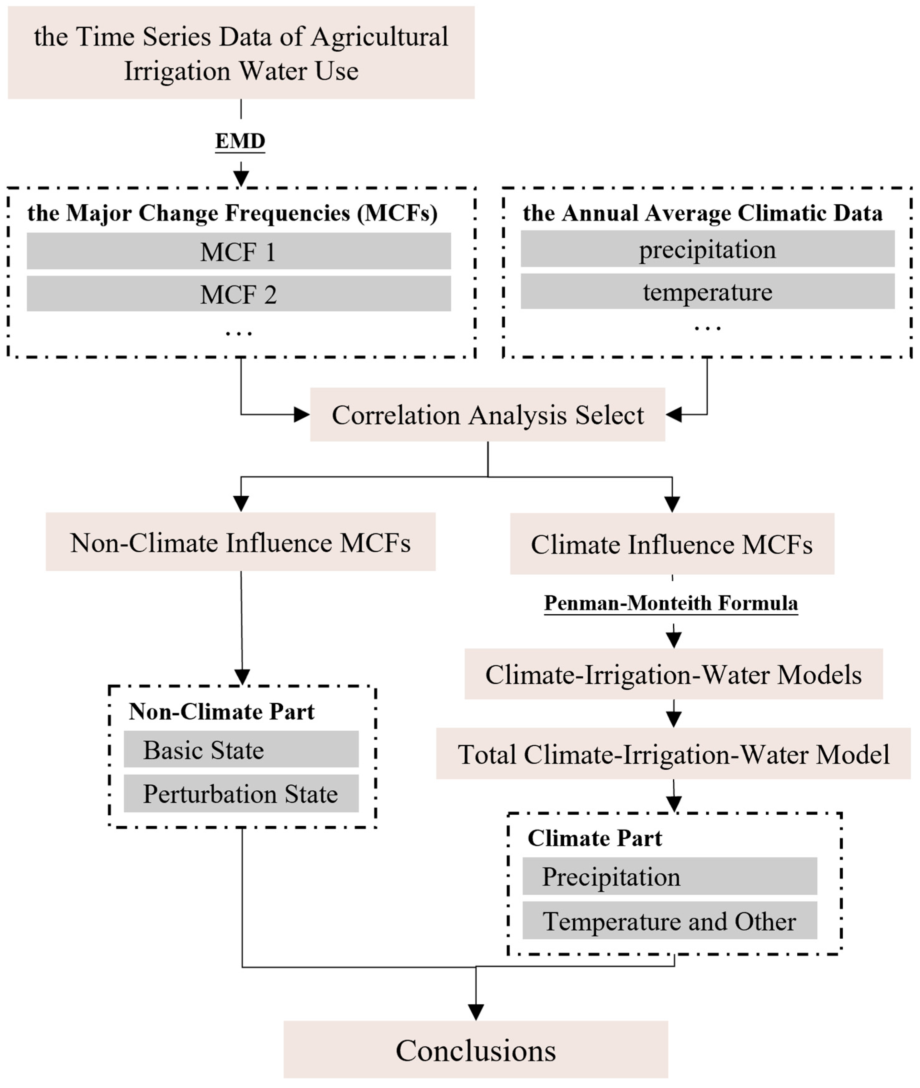
2.3. Method Overview

The analysis process is illustrated in Figure 1. Initially, the Empirical Mode Decomposition (EMD) technique was applied to dissect the time-series data of irrigation water use, revealing the significant change frequencies. Subsequently, through correlation analysis and statistical testing, the key change frequencies susceptible to climatic influences were identified. Using the Penman–Monteith formula as a foundation, distinct climatic models for irrigation water use were formulated corresponding to each selected significant change frequency. Ultimately, an overarching climatic irrigation water use model was established by integrating all the individual models, offering a comprehensive representation of the impact of climate factors. Concurrently, the change frequencies not influenced by climate factors were attributed to non-climate forces. Within the non-climate segment, a division was made between the basic and perturbation states for further analysis.

2.4. Data Analysis Method

2.4.1. Empirical Mode Decomposition

EMD is a sequence data analysis method. Any data sequence can be split into the sum of several Intrinsic Mode Functions (IMF), where it must satisfy the two constraints, as given in Equation (1).
P o i n t e P o i n t z   1 e m a x x + e m i n ( x ) 2 = 0
where P o i n t e and P o i n t z are the extreme points and zero points on the IMF curve, e m a x x is an upper envelope constructed by the spline interpolation of IMF maximum points, and e m a x x is the lower envelope constructed by the spline interpolation of IMF minimum points.
The process of using EMD for sequence data f ( x ) is given below:
(1) Find all extreme points of f ( x ) . Use cubic spline interpolation method to fit the maximum points to the upper envelope e m a x x and the minimum points to the lower envelope e m i n ( x ) .
(2) Use Equation (2) to calculate the average curve m 1 ( x ) . The intermediate sequence data C 1,1 ( x ) is decomposed out, as in Equation (3)
m 1 x = e m a x x + e m i n ( x ) 2
C 1,1 x = f x m 1 x
(3) Determine whether the intermediate sequence data C 1,1 ( x ) satisfies Equation (1). If it satisfies the condition, it is an IMF; otherwise, use C 1,1 ( x ) and repeat steps 1 and 2 until the C 1 , k x , which is obtained after k times of calculations and satisfies the constraint condition. Then, take C 1 , k ( x ) as i m f 1 ( x ) .
(4) Use Equation (4) to calculate the remaining sequence of data f 2 ( x ) ; for f 2 ( x ) , repeat steps 1, 2, 3 and 4 until f 2 ( x ) is a monotonic sequence. Finally, the original sequence data f ( x ) are decomposed into n IMF parts and residual part, f n ( x ) , as Equation (5).
f 2 x = f x i m f 1
f x = i = 1 n i m f i x + f n x

2.4.2. Correlation and Testing Method

The Pearson correlation coefficient R [42] was used to analyze the correlation between climatic factors and irrigation water use. The higher the absolute value of R , the stronger the correlation. Equation (6) presents the Pearson correlation formula.
R = i = 1 m ( x i x ¯ ) ( y i y ¯ ) i = 1 m ( x i x ¯ ) 2 i = 1 m ( y i y ¯ ) 2
where x i is a certain climate factor, x ¯ is the average value of climate factor, y i is irrigation water use, y ¯ is the average value of irrigation water use, and m is the sample size.
There are a variety of statistical tests for calculating the significance level, p-value. It refers to the probability that the hypothesis, in which the real correlation is zero according to the correlation coefficient R, is true. Namely, when the samples x and y conform to the normal distribution, the probability density function of the correlation coefficient R distribution is Equation (7). The p-value is calculated using Equation (8). Generally, the smaller the p-value is, the more significant the correlation is. In this paper, 0.05 and 0.01 are used as the standard for assessing the significance of the correlation.
f R = 1 R 2 m / 2 2 B ( 1 2 , m 2 1 )
P = R R f R d R
R is the correlation coefficient, m is the sample size, and B is the beta distribution.

2.4.3. Irrigation-Water-Use Model and Evaluation

The irrigation water requirement (IWR) and the climate factor have an approximate relationship in Equation (9), defined by FAO [22].
I W R = i = 1 n E T c i P e · A r e a i
where I W R is the irrigation water requirement (m3), A r e a i is the crop planting area (m2), P e is the effective precipitation (mm), E T c i is the actual total evapotranspiration of crops (mm), and n is the number of crops.
In actual irrigation, the actual irrigation water use is not equivalent to IWR due to the irrigation method. So, we describe the relationship between IWR and irrigation water use by introducing a coefficient ε (Equation (10)), a region-specific parameter influenced by the regional irrigation method and irrigation efficiency.
A I W U = ε × I W R
where A I W U is the irrigation water use. According to the Penman–Monteith formula, it is known that
E T c ( T , W s , 1 R h , 1 V p )
where T is the average air temperature (°C), W s is the average wind speed ( m · s 1 ), R h is the relative humidity, and V p is the water vapor pressure (hPa). Equation (12) can be obtained from Equations (9)–(11)
A I W U 1 P , T , W s , 1 R h , 1 V p
That is, in the irrigation region, the A I W U is proportional to the average temperature T and average wind speed, W s , and inversely proportional to the precipitation P , relative humidity R h and water vapor pressure, V p .
Based on the above analysis process, a statistical model of Equation (13) can be built to describe the relationship between climate factors and irrigation water use.
A I W U ^ = k T W s P R h V p + b
where A I W U ^ is the irrigation water use fitted by the model, and k and b are empirical coefficients.
Sometimes, this irrigation water use model (Equation (13)) should be optimized and adjusted if some climate elements may not have a significant correlation with the irrigation water use. For example, if the correlation between the wind speed ( W s ) and the irrigation water use is not significant, W s will be infinitely close to 1. Then, the irrigation water use model will be Equation (14). Finally, the empirical coefficients k and b are obtained by the least-squares method.
A I W U ^ = k T P R h V p + b
Equation (15) is used to calculate the root mean square error (RMSE) to describe the built model’s accuracy.
R M S E = i = 1 n ( x i x ^ i ) 2 n
where x i is the true value, x ^ i is the model simulated value, and n is the sample size.

2.4.4. Data Analysis Tools

In this paper, Python 3.7 [43] was used for the calculation and data analysis. The tripartite libraries used were NumPy 1.21.6 [44], Pandas 1.3.0 [45], PyEMD 0.2.7 [46,47], SciPy 1.7.3 [48], scikit-learn 0.23.1 [49] and Matplotlib 3.5.2 [50].

3. Results

3.1. Characteristics of Climate Factors Change

The distribution of climatic factors in Jiangsu Province from 2004 to 2020 is shown in Figure 2. The annual average ± standard deviation of precipitation was 1034.4 ± 156.6 mm, with a fluctuation range of −24–36% (Figure 2a). The precipitation was less in 2004, 2013 and 2019 (784.3, 833.4 and 798.5 mm, respectively). The highest precipitation was 1410.5 mm in 2016.
Figure 2b shows the air temperature variation. The multi-year average ± standard deviation of air temperature was 16.1 °C. The temperature was the lowest in 2011 (15.4 °C) and the highest in 2007 and 2017 (16.7 and 16.6 °C). Based on linear regression, it showed a trend of “decrease-increase”. Specifically, there was a decrease rate of 0.11 °C/year from 2004 to 2011 (p < 0.05), and an increase rate of 0.13 °C/year during the period from 2011 to 2020 (p < 0.05).
The multi-year average ± standard deviation of wind speed (Figure 2c) was 2.7 ± 0.2 m · s 1 . The highest wind speed was 2.7 m · s 1 in 2005, and the lowest was 2.6 m · s 1 in 2015. The linear fitting showed a decreasing wind speed trend by 0.02 m · s 1 /year.
The trend in relative humidity (Figure 2d) was consistent with the water vapor pressure (Figure 2e). The multi-year average ± standard deviation of relative humidity was 74 ± 2%, changing between 70% (2011) and 77% (2020). The average water vapor pressure fluctuated from 14.5 hPa in 2011 to 16.6 hPa in 2018, with an average ± standard deviation of 15.5 ± 0.6 hPa. The linear fitting analysis revealed that during the period of 2004–2011, both the relative humidity and water vapor pressure exhibited a declining trend, with a decrease rate of 0.4% and 0.1 hPa (p < 0.05). However, in the subsequent period of 2011–2020, both climatic elements showed an increasing trend, with an increase rate of 1% and 0.2 hPa (p < 0.05), respectively.

3.2. Characteristics of Irrigation Water Use Change

Figure 3a shows the irrigation water use variation in Jiangsu Province from 2004 to 2020. The average annual irrigation water use was 25.44 billion m3, with a maximum of 27.38 billion m3 in 2011 and a minimum of 23.96, 23.87 and 23.72 billion m3 in 2005, 2007 and 2016, respectively. The irrigation water use showed an “increases-decrease-increase” trend. It gradually increased in 2005–2011 with a rate of 650.00 million m3/year (Mann–Kendall test was 0.81, p < 0.01), then decreased in 2011–2016 with a rate of 750.00 million m3/year (Mann–Kendall test was −0.99, p < 0.01), and finally increased again in 2016–2019 with the rate of 942.00 million m3/year but the increase was not significant (Mann–Kendall test was 0.67, p > 0.01).
The calculation of the irrigation water use series based on the EMD is depicted in Figure 3b. There were three main change frequencies for irrigation water use, namely MCF1, MCF2 and MCF3. The MCF1 (Figure 3(b1)) was a 2-to-3-year period varied over a ±1.00 billion m3 range. It exhibited significant fluctuations during 2004–2007 and 2016–2020, while remaining relatively stable during the other years. The MCF2 (Figure 3(b2)) varied over a ±2.00 billion m3 range throughout 10 years. There was a complete cycle change during 2006–2016. Simultaneously, the amplitude of this cyclic variation gradually decreased. For instance, the lowest amplitude in 2006 was −1.84 billion m3, while it was −1.09 billion m3 in 2016, with an overall declining rate of 0.08 billion m3/year. The MCF3 (Figure 3(b3)) exhibited a consistent decreasing pattern, declining from 25.67 billion m3 to 24.76 billion m3 between 2004 and 2020. It also showed that the irrigation water use generally had a downward trend with a decreasing rate of 0.05 billion m3/year.

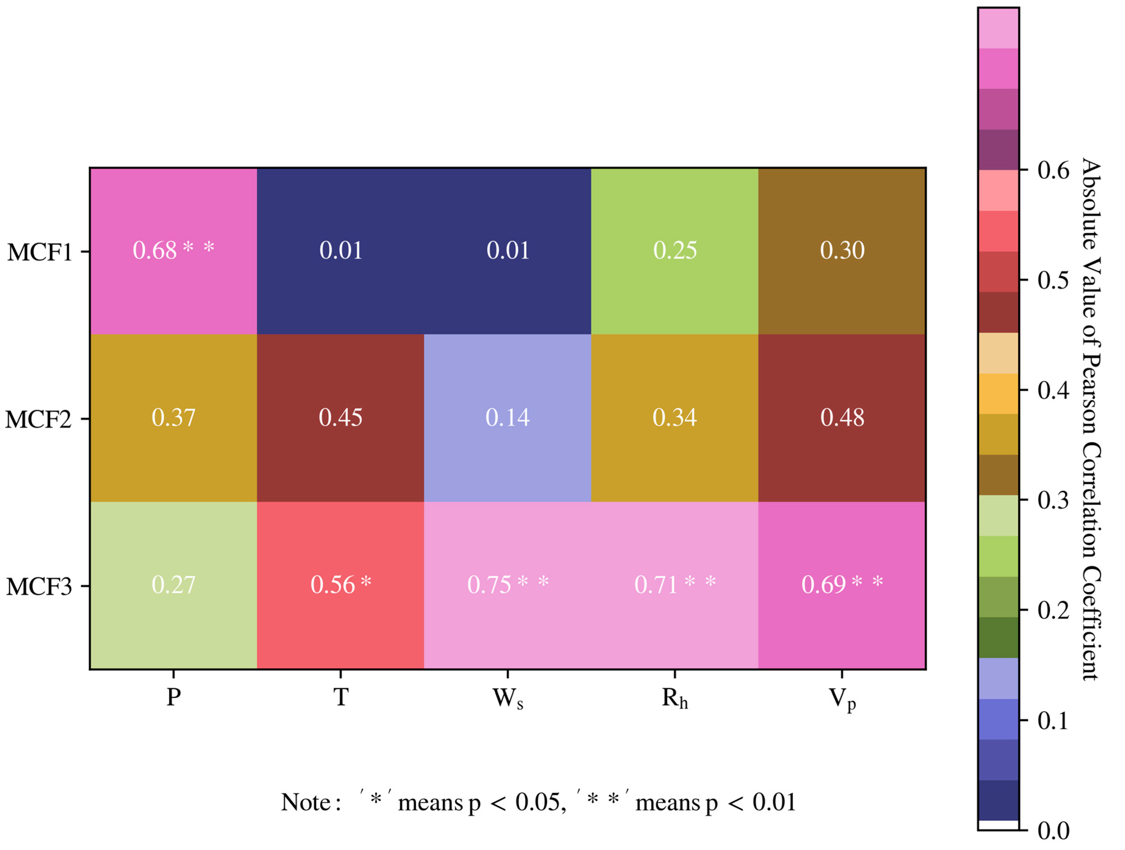
3.3. Relationship between Climatic Factors and Irrigation Water Use

The correlation between climatic factors and MCF1, MCF2, and MCF3 is presented in Figure 4. The findings indicated that precipitation exhibited the highest correlation with MCF1, with a Pearson correlation coefficient of 0.68, and this correlation was statistically significant (p < 0.05). Air temperature, wind speed, relative humidity, and water vapor pressure had correlation coefficients of 0.56, 0.75, 0.71, and 0.69, respectively, with MCF3, all of which were significant at a p < 0.05 level. However, the relationship between MCF2 and these climate factors was weak and non-significant, implying that non-climatic factors potentially influenced MCF2.

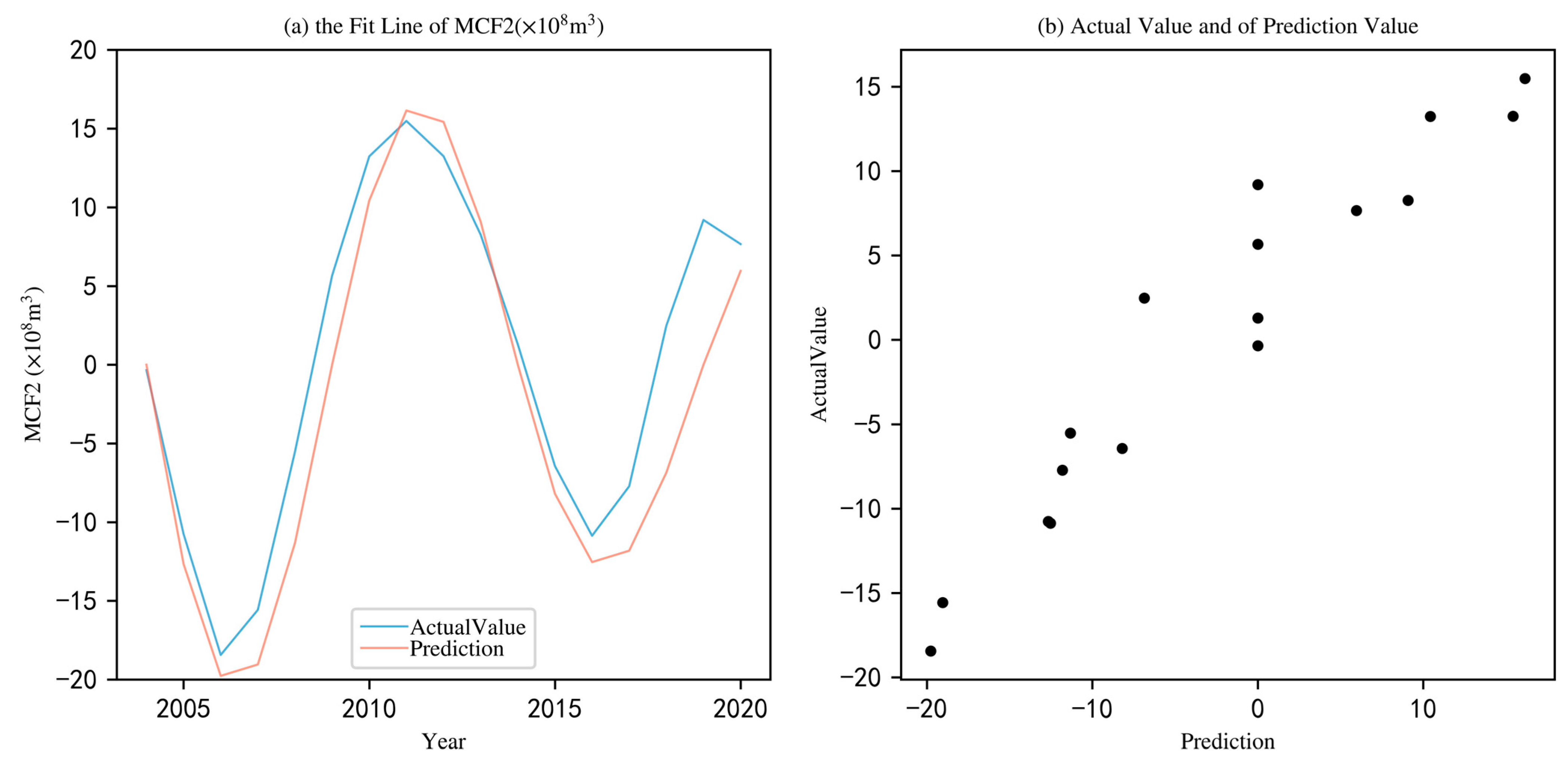
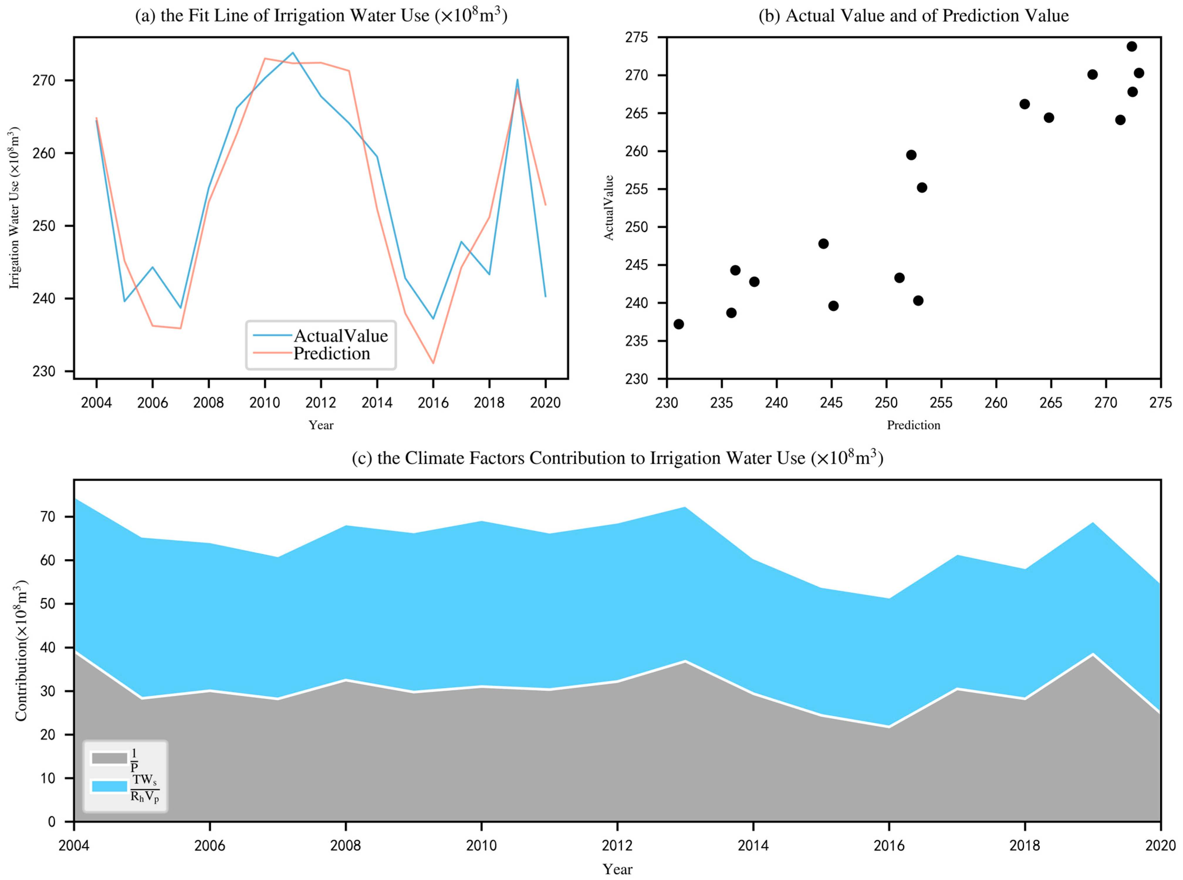
3.4. Climate–Irrigation–Water Model

According to the analysis in Section 2, Equation (16) can be concluded.
A I W U = M C F 1 + M C F 2 + M C F 3
where A I W U is the irrigation water use, and M C F 1 , M C F 2 , and M C F 3 are the first, second, and third major change frequencies, respectively. The relationship between MCFs and climate factors is described by the following model (Equation (17)).
M C F 1 = k 1 T W s P R h V p + b 1 M C F 2 = k 2 T W s P R h V p + b 2 M C F 3 = k 3 T W s P R h V p + b 3
Based on the analysis presented in Section 3.3, the M C F 1 was only related to the precipitation, while M C F 3 was related to air temperature, wind speed, relative humidity, and water vapor pressure. So, let the irrelevant items in the formula tend to 1, which reduces Equation (17) to
M C F 1 = k 1 1 P + b 1 M C F 3 = k 3 T W s R h V p + b 3
The parameters in Equation (18) were solved using the least-squares algorithm. Then, based on the superposition of individual models, the Climate–Irrigation–Water Model was obtained, as shown in Equation (19). The fitting effect R2 of M C F 1 was 0.50, and the fitting effect R2 of M C F 3 was 0.68.
A I W U ^ = 30725.15 P + 961.99 T W s R h V p + M C F 2 + 190.43
The estimated irrigation water use using Equation (19) is shown in Figure 5. The results showed that the trend in irrigation water use simulated by Equation (19) was consistent with the observed trend. The time-series plot in Figure 5a indicated a good simulation of the real change in irrigation water use. A scatter plot of the simulated and true irrigation water use showed that the points were evenly distributed around the 1:1 line (Figure 5b). The model’s RMSE was 0.06 billion m3, accounting for 2.24% of the average irrigation water use. It means a lower model error and better simulation of irrigation water use.
The Climate–Irrigation–Water Model (Equation (19)) shows that it consists of four items: the first two items 30725.15 P and 961.99   T   W s R h   V p are related to climatic factors, the third item MCF2 is related to non-climatic factors, and the fourth item is constant. Contributions of items related to climate elements to irrigation water use are shown in Figure 5c. The outcomes indicated that the average contribution of precipitation to irrigation water use amounted to 3.04 billion m3, equivalent to 11.94%. This contribution displayed considerable fluctuation (with a standard deviation of 452.00 million m3), particularly during the period from 2013 to 2020. Moreover, the average contribution of other climatic components, such as temperature and wind speed, stood at 3.36 billion m3, making up 13.20%. This contribution exhibited relatively gradual variations, with a standard deviation of 299.00 million m3. A minor fluctuation was observed from 2004 to 2011.

4. Discussion

In this paper, we developed a Climate–Irrigation–Water Model based on the theory of farmland irrigation and the EMD method. It is crucial not to overlook either the theory of farmland irrigation or the EMD method. Ignoring the theory of farmland irrigation may result in noticeable errors when analyzing the impact of climate change on irrigation water use. For example, considering only the linear relationship between climatic factors and irrigation water use would oversimplify the model.
A I W U ^ = 0.05 P 4.23 T 17.40 W s + 0.92 R h 14.13 V p + 568.12
Furthermore, Equation (20) showed a negative linear correlation between A I W U ^ and T . It meant that as the temperature increases, the irrigation water use will be greatly reduced, contrary to the previous studies [51,52,53]. On the other hand, if the model were solely constructed based on the theory of farmland irrigation, it would be expressed as follows.
A I W U ^ = θ T W s P R h V p + 206.03
where the θ parameter is
θ = 1.4 × 10 6
when the farmland irrigation theory was used as the basis, the model structure of Equation (21) was more reasonable, and the relationship between the irrigation water use and climatic factors was clearer. But, its RMSE was 0.09 billion m3, which was 50.00% more than the model built by the theory of farmland irrigation and the EMD method together (Equation (19)).
The unreasonable error of Equations (20) and (21) models was not considering non-climatic factors. Climatic and non-climatic factors such as irrigation area, planting structure, and irrigation efficiency influence the actual irrigation water. Therefore, constructing a model solely based on climatic factors is unreasonable and inaccurate. This paper utilized the EMD to analyze the major change frequencies of irrigation water use. The trends of each major change frequency were apparent, and the impact of climate elements on these frequencies was intuitively determined, allowing for the development of a more reasonable and accurate model.
The final model (Equation (19)) revealed that irrigation water use consists of four components, two of which were influenced by climate factors, while non-climatic factors influenced the other two. For the climate-related components, the first part is primarily influenced by precipitation, while the second part is affected by the combined effects of temperature, wind speed, and water vapor pressure. The model’s structure aligns closely with the findings of the FAO. According to the model, the contribution of climate factors to irrigation water fluctuates around 6.40 billion m3, accounting for 25.14% of the total irrigation water, which is consistent with the results obtained by Fischer G et al. [54] and De Silva C S et al. [55]. Notably, the contribution experienced significant fluctuations from 2013 to 2020, primarily driven by the first part related to precipitation. In contrast, the contribution shows slight variations during 2004–2011, primarily influenced by the second part associated with temperature and other climate factors (Figure 5c).
In contrast, the non-climatic components of the model consist of MCF2 and the constant term. The constant term has a value of 20.60 billion m3, representing the average amount of irrigation water use in Jiangsu Province from 2004 to 2020 without the influence of climate factors. This value refers to the basic irrigation water use (BAIWU), which represents the average state based on the analysis of irrigation water use during the years 2004–2020. The BAIWU is primarily influenced by various factors in Jiangsu, including average irrigation area, average planting structure, average irrigation efficiency, and others. Since the BAIWU reflects the average state between 2004 and 2020, its value is unlikely to change in the near future (5–15 years). However, it may be subject to alteration due to unforeseen factors in the distant future.
The MCF2 part, which changes between −2.00 and 2.00 (billion m3), is the perturbation at the state, that is, the perturbation of irrigation water use (PAIWU). The PAIWU is caused by small human-made adjustments in agricultural production between years. Here is a simple example to illustrate the concept. In the first year, the rice cultivation area increased due to market demand, resulting in an increased irrigation water requirement. However, in the second year, there was a reduction in cultivated land area due to urbanization, leading to a decrease in irrigation water. This disturbance process typically occurs over a longer period in reality. In summary, the PAIWU is primarily attributed to the continuous accumulation of small positive and negative human influences. Fortunately, the analysis of the disturbance amplitude of MCF2 shows that the complex and uncontrollable human influence is gradually diminishing over time, with a decreasing rate of 0.08 billion m3 per year. Equation (21) was developed based on the data analysis of MCF2 to reflect the changes in PAIWU over time.
M C F 2 t = max 0 ,   22.30 0.76 t sin π 5 t + 5
where t is
t = Y e a r 2004
Figure 6a shows the variation of the disturbance irrigation water simulated by Equation (22), and Figure 6b shows a scatterplot of true and fitted values. The results showed that M C F 2 t could fit the variation of the PAIWU well, and the simulation and true scatter plots were evenly distributed on the 1:1 line. Further analysis of Equation (22) showed that the PAIWU decreased gradually over time and might be negligible after 20 years in the future.
This paper aimed to analyze the changes in irrigation water use on different time scales. In addition, it analyzed the influence of various climatic elements on it. Finally, an irrigation-water-use simulation model was developed. The results provided some reference and research basis for the subsequent study of irrigation water use. There are still some parts in the paper that need further analysis in the future: (1) For this paper, our main purpose was to try to propose a new method and direction for building the Climate–Irrigation–Water Model. So, based on the evapotranspiration theory, we only considered the simple relationship between climatic elements and irrigation water use. In fact, more details should be considered to improve the model`s accuracy and rationality. For example, the Climate–Irrigation–Water Model should further consider the constraints of climatic elements. (2) The impacts of human factors on irrigation demand, such as planting area, planting structure, water-saving factors, etc., still need to be analyzed for future irrigation water change.

5. Conclusions

This paper analyzed the climatic factors and irrigation water use in Jiangsu Province during 2004–2020 by the Empirical Mode Decomposition method. Here are some conclusions:
(1) The annual means ± standard deviation of irrigation water use, precipitation, air temperature, wind speed, relative humidity and vapor pressure were 25.44 ± 1.28 billion m3, 1034.4 ± 156.6 mm, 16.1 ± 0.4 °C, 2.7 ± 0.2 m · s 1 , 74 ± 2%, and 15.5 ± 0.6 hPa, respectively. (2) Based on the EMD method, it showed that the irrigation water use had three main change frequencies (MCF1, MCF2 and MCF3). The MCF1 was a 2-to-3-year period varied over a ±1.00 billion m3 range. The MCF2 was varied over a ±2.00 billion m3 range throughout 10 years. The MCF3 showed a downward trend with a rate of 0.05 billion m3/year. The correlation analysis showed that the MCF1 was influenced by the precipitation (the Pearson correlation was 0.68, p < 0.05). At the same time, the MCF3 was comprehensively impacted by temperature, wind speed, relative humidity, and water vapor pressure (the Pearson correlations were 0.56, 0.75, 0.71, and 0.69, respectively, p < 0.05). (3) Then, based on the correlation selection and the farmland irrigation theory, the Climate–Irrigation–Water Model was developed. Its root mean square error (RMSE) was 0.06 billion m3, accounting for 2.24%, and the simulation was accurate. It revealed that the average impact of climate factors on agricultural irrigation water use was 6.40 billion m3, accounting for 25.14%, of which the impact of precipitation was 3.04 billion m3, and the comprehensive impact of other climatic factors was 3.36 billion m3.
Nevertheless, future research priorities remain ahead to enhance further and continue the irrigation water use study. (1) When constructing the Climate–Irrigation–Water Model, it is essential to consider more details. For example, the model should further consider the constraints of climatic elements. (2) The impacts of human factors on irrigation water use, such as planting area, planting structure, water-saving factors, etc., still need to be analyzed.

Author Contributions

All authors contributed to the study’s conception and design. Data collection was carried out by T.Z., X.W. and Z.J. Data analyses were performed by T.Z., B.B., X.W., T.Z. and X.W. wrote the first draft of the manuscript. The final draft was reviewed and written by X.W., T.Z., Z.J., S.S. and B.B. All authors have read and agreed to the published version of the manuscript.

Funding

The study was supported by National Natural Science Foundation of China (No. 52121006), Young Top-Notch Talent Support Program of National High-level Talents Special Support Plan, Research Project of Ministry of Natural Resources (No. 20210103), Research Project of Jiangsu Provincial Department of Natural Resources (No. 2021003, 2022022), Research Project of Jiangsu Land and Resources Research Center (No. 2020TDZY06, ZK202106, ZK22003), Research Project of Taizhou Municipal Bureau of Natural Resources and Planning (No. TZC2022071-jssydl), Six Talents Peak Project of Jiangsu Province (No. JNHB-068), 333 High-level Talents Cultivation Project of Jiangsu Province and Research Project of Jiangsu Water Conservancy Research Institute (No. 2022019). We are also thankful to anonymous reviewers and editors for their helpful comments and suggestions.

Institutional Review Board Statement

The manuscript complies with all the ethical requirements; the paper was not submitted to any other journal. All the sources and contributors were acknowledged properly.

Informed Consent Statement

All authors consent to the publication.

Data Availability Statement

The datasets generated during and/or analyzed during the current study are available in Xiaojun Wang et al.

Conflicts of Interest

The authors declare no conflict of interest.

References

  1. Stocker, T. (Ed.) Climate Change 2013: The Physical Science Basis: Working Group I Contribution to the Fifth Assessment Report of the Intergovernmental Panel on Climate Change; Cambridge University Press: Cambridge, UK, 2014. [Google Scholar]
  2. Cook, J.; Oreskes, N.; Doran, P.T.; Anderegg, W.R.; Verheggen, B.; Maibach, E.W.; Carlton, J.S.; Lewandowsky, S.; Skuce, A.G.; Green, S.A.; et al. Consensus on consensus: A synthesis of consensus estimates on human-caused global warming. Environ. Res. Lett. 2016, 11, 048002. [Google Scholar] [CrossRef]
  3. Putnam, A.E.; Broecker, W.S. Human-induced changes in the distribution of rainfall. Sci. Adv. 2017, 3, e1600871. [Google Scholar] [CrossRef]
  4. Vautard, R.; Gobiet, A.; Jacob, D.; Belda, M.; Colette, A.; Déqué, M.; Fernández, J.; García-Díez, M.; Goergen, K.; Güttler, I.; et al. The simulation of European heat waves from an ensemble of regional climate models within the EURO-CORDEX project. Clim. Dyn. 2013, 41, 2555–2575. [Google Scholar] [CrossRef]
  5. Piao, S.; Ciais, P.; Huang, Y.; Shen, Z.H.; Peng, S.S.; Li, J.S.; Zhou, L.P.; Liu, H.Y.; Ma, Y.C.; Ding, Y.H.; et al. The impacts of climate change on water resources and agriculture in China. Nature 2010, 467, 43–51. [Google Scholar] [CrossRef] [PubMed]
  6. Grusson, Y.; Wesström, I.; Joel, A. Impact of climate change on Swedish agriculture: Growing season rain deficit and irrigation need. Agric. Water Manag. 2021, 251, 106858. [Google Scholar] [CrossRef]
  7. Shrestha, A.B.; Agrawal, N.K.; Alfthan, B.; Bajracharya, S.R.; Maréchal, J.; Oort, B.V. The Himalayan Climate and Water Atlas: Impact of Climate Change on Water Resources in Five of Asia’s Major River Basins; ICIMOD: Patan, Nepal, 2015. [Google Scholar]
  8. Jeuland, M.; Harshadeep, N.; Escurra, J.; Blackmore, D.; Sadoff, C. Implications of climate change for water resources development in the Ganges basin. Water Policy 2013, 15, 26–50. [Google Scholar] [CrossRef]
  9. Mishra, V.; Kumar, R.; Shah, H.L.; Samaniego, L.; Eisner, S.; Yang, T. Multimodel assessment of sensitivity and uncertainty of evapotranspiration and a proxy for available water resources under climate change. Clim. Chang. 2017, 141, 451–465. [Google Scholar] [CrossRef]
  10. Abdelhafez, A.A.; Metwalley, S.M.; Abbas, H.H. Irrigation: Water Resources, Types and Common Problems in Egypt. In Technological and Modern Irrigation Environment in Egypt; Springer: Cham, Switzerland, 2020; pp. 15–34. [Google Scholar]
  11. Rasul, G. Twin challenges of COVID-19 pandemic and climate change for agriculture and food security in South Asia. Environ. Chall. 2021, 2, 100027. [Google Scholar] [CrossRef]
  12. Sunil, A.; Deepthi, B.; Mirajkar, A.B.; Adarsh, S. Modeling future irrigation water demands in the context of climate change: A case study of Jayakwadi command area, India. Model. Earth Syst. Environ. 2021, 7, 1963–1977. [Google Scholar] [CrossRef]
  13. Uniyal, B.; Dietrich, J.; Vu, N.Q.; Jha, M.K.; Arumí, J.L. simulation of regional irrigation requirement with SWAT in different agro-climatic zones driven by observed climate and two reanalysis datasets. Sci. Total Environ. 2019, 649, 846–865. [Google Scholar] [CrossRef]
  14. Goodarzi, M.; Abedi-Koupai, J.; Heidarpour, M. Investigating impacts of climate change on irrigation water demands and its resulting consequences on groundwater using CMIP5 models. Groundwater 2019, 57, 259–268. [Google Scholar] [CrossRef]
  15. Watson, J.; Zheng, B.; Chapman, S.; Chenu, K. Projected impact of future climate on water-stress patterns across the Australian wheatbelt. J. Exp. Bot. 2017, 68, 5907–5921. [Google Scholar] [CrossRef] [PubMed]
  16. Wang, W.; Sun, F.; Luo, Y.; Xu, J. Changes of rice water demand and irrigation water requirement in Southeast China under future climate change. Procedia Eng. 2012, 28, 341–345. [Google Scholar] [CrossRef]
  17. Christy, B.; Tausz-Posch, S.; Tausz, M.; Richards, R.; Rebetzke, G.; Condon, A.; McLean, T.; Fitzgerald, G.; Bourgault, M.; O’Leary, G. Benefits of increasing transpiration efficiency in wheat under elevated CO2 for rainfed regions. Glob. Chang. Biol. 2018, 24, 1965–1977. [Google Scholar] [CrossRef] [PubMed]
  18. Lee, J.L.; Huang, W.C. Impact of climate change on the irrigation water requirement in Northern Taiwan. Water 2014, 6, 3339–3361. [Google Scholar] [CrossRef]
  19. Rehana, S.; Mujumdar, P.P. Regional impacts of climate change on irrigation water demands. Hydrol. Process. 2013, 27, 2918–2933. [Google Scholar] [CrossRef]
  20. Gorguner, M.; Kavvas, M.L. Modeling impacts of future climate change on reservoir storages and irrigation water demands in a Mediterranean basin. Sci. Total Environ. 2020, 748, 141246. [Google Scholar] [CrossRef] [PubMed]
  21. Khaydar, D.; Chen, X.; Huang, Y.; Ilkhom, M.; Liu, T.; Friday, O.; Farkhod, A.; Khusen, G.; Gulkaiyr, O. Investigation of crop evapotranspiration and irrigation water requirement in the lower Amu Darya River Basin, Central Asia. J. Arid Land 2021, 13, 23–39. [Google Scholar] [CrossRef]
  22. Beven, K. A sensitivity analysis of the Penman-Monteith actual evapotranspiration estimates. J. Hydrol. 1979, 44, 169–190. [Google Scholar] [CrossRef]
  23. Wang, X.; Zhang, J.; Ali, M.; Shahid, S.; He, R.-M.; Xia, X.-H.; Jiang, Z. impact of climate change on regional irrigation water demand in Baojixia irrigation district of China. Mitig. Adapt. Strateg. Glob. Chang. 2016, 21, 233–247. [Google Scholar] [CrossRef]
  24. Perea, R.G.; Ballesteros, R.; Ortega, J.F.; Moreno, M. Water and energy demand forecasting in large-scale water distribution networks for irrigation using open data and machine learning algorithms. Comput. Electron. Agric. 2021, 188, 106327. [Google Scholar] [CrossRef]
  25. Weiler, M.; Beven, K. Do we need a community hydrological model? Water Resour. Res. 2015, 51, 7777–7784. [Google Scholar] [CrossRef]
  26. Addor, N.; Melsen, L.A. Legacy, rather than adequacy, drives the selection of hydrological models. Water Resour. Res. 2019, 55, 378–390. [Google Scholar] [CrossRef]
  27. Fang, Q.X.; Green, T.R.; Ma, L.; Erskine, R.H.; Malone, R.W.; Ahuja, L.R. Optimizing soil hydraulic parameters in RZWQM2 under fallow conditions. Soil Sci. Soc. Am. J. 2010, 74, 1897–1913. [Google Scholar] [CrossRef]
  28. Kauffeldt, A.; Wetterhall, F.; Pappenberger, F.; Salamon, P.; Thielen, J. Technical review of large-scale hydrological models for implementation in operational flood forecasting schemes on continental level. Environ. Model. Softw. 2016, 75, 68–76. [Google Scholar] [CrossRef]
  29. Haddeland, I.; Clark, D.B.; Franssen, W.; Ludwig, F.; Voß, F.; Arnell, N.W.; Bertrand, N.; Best, M.; Folwell, S.; Gerten, D.; et al. Multimodel estimate of the global terrestrial water balance: Setup and first results. J. Hydrometeorol. 2011, 12, 869–884. [Google Scholar] [CrossRef]
  30. Huang, N.E.; Shen, Z.; Long, S.R.; Wu, M.C.; Shih, H.H.; Zheng, Q.; Yen, N.-C.; Tung, C.C.; Liu, H.H. The Empirical Mode Decomposition and the Hilbert Spectrum for Nonlinear and Non-stationary Time Series Analysis. Proc. R. Soc. London. Ser. A Math. Phys. Eng. Sci. 1998, 454, 903–995. [Google Scholar] [CrossRef]
  31. Zeiler, A.; Faltermeier, R.; Keck, I.R.; Tomé, A.M. Empirical Mode Decomposition-An Introduction. In Proceedings of the 2010 International Joint Conference on Neural Networks (IJCNN), Barcelona, Spain, 18–23 July 2010; IEEE: Piscataway, NJ, USA, 2010; pp. 1–8. [Google Scholar]
  32. Ur Rehman, N.; Mandic, D.P. Filter bank property of multivariate empirical mode decomposition. IEEE Trans. Signal Process. 2011, 59, 2421–2426. [Google Scholar] [CrossRef]
  33. Li, H.; Li, Z.; Mo, W. A time varying filter approach for empirical mode decomposition. Signal Process. 2017, 138, 146–158. [Google Scholar] [CrossRef]
  34. Kabir, M.A.; Shahnaz, C. Denoising of ECG signals based on noise reduction algorithms in EMD and wavelet domains. Biomed. Signal Process. Control 2012, 7, 481–489. [Google Scholar] [CrossRef]
  35. Huang, S.; Chang, J.; Huang, Q.; Chen, Y. Monthly streamflow prediction using modified EMD-based support vector machine. J. Hydrol. 2014, 511, 764–775. [Google Scholar] [CrossRef]
  36. Sang, Y.F.; Wang, Z.; Liu, C. Comparison of the MK test and EMD method for trend identification in hydrological time series. J. Hydrol. 2014, 510, 293–298. [Google Scholar] [CrossRef]
  37. Tan, Q.F.; Lei, X.H.; Wang, X.; Wang, H.; Wen, X.; Ji, Y.; Kang, A.Q. An adaptive middle and long-term runoff forecast model using EEMD-ANN hybrid approach. J. Hydrol. 2018, 567, 767–780. [Google Scholar] [CrossRef]
  38. Libanda, B.; Nkolola, N.B. An ensemble empirical mode decomposition of consecutive dry days in the Zambezi Riparian Region: Implications for water management. Phys. Chem. Earth Parts A/B/C 2022, 126, 103147. [Google Scholar] [CrossRef]
  39. Jiangsu Provincial Bureau of Statistics. Jiangsu Statistical Yearbook; China Statistics Press: Beijing, China, 2022. [Google Scholar]
  40. Jiangsu Provincial Department of Water Resources. Jiangsu Water Resources Bulletin 2004–2021; Water Resources Department of Jiangsu Province Press: Jiangsu, China, 2004–2021.
  41. China Meteorological Data Network. National Meteorological Science Data Center. Available online: https://data.cma.cn/ (accessed on 20 February 2023).
  42. Pearson Correlation Coefficient. Wikipedia. Available online: https://en.wikipedia.org/wiki/Pearson_correlation_coefficient (accessed on 20 February 2023).
  43. Van Rossum, G.; Drake, F.L. Python 3 Reference Manual; CreateSpace: Scotts Valley, CA, USA, 2009. [Google Scholar]
  44. Harris, C.R.; Millman, K.J.; Van Der Walt, S.J.; Gommers, R.; Virtanen, P.; Cournapeau, D.; Wieser, E.; Taylor, J.; Berg, S.; Smith, N.J.; et al. Array programming with NumPy. Nature 2020, 585, 357–362. [Google Scholar] [CrossRef] [PubMed]
  45. McKinney, W. Data Structures for Statistical Computing in Python. In Proceedings of the 9th Python in Science Conference, Austin, TX, USA, 28 June–3 July 2010; Volume 445, pp. 51–56. [Google Scholar]
  46. Pele, O.; Werman, M. A Linear Time Histogram Metric for Improved Sift Matching. In European Conference on Computer Vision; Springer: Berlin/Heidelberg, Germany, 2008; pp. 495–508. [Google Scholar]
  47. Pele, O.; Werman, M. Fast and Robust Earth Mover’s Distances. In Proceedings of the 2009 IEEE 12th International Conference on Computer Vision, Kyoto, Japan, 29 September–2 October 2009; IEEE: Piscataway, NJ, USA, 2009; pp. 460–467. [Google Scholar]
  48. Virtanen, P.; Gommers, R.; Oliphant, T.E.; Haberland, M.; Reddy, T.; Cournapeau, D.; Burovski, E.; Peterson, P.; Weckesser, W.; Bright, J.; et al. SciPy 1. 0: Fundamental algorithms for scientific computing in Python. Nat. Methods 2020, 17, 261–272. [Google Scholar]
  49. Pedregosa, F.; Varoquaux, G.; Gramfort, A.; Michel, V.; Thirion, B.; Grisel, O.; Blondel, M.; Prettenhofer, P.; Weiss, R.; Dubourg, V.; et al. Scikit-learn: Machine learning in Python. J. Mach. Learn. Res. 2011, 12, 2825–2830. [Google Scholar]
  50. Hunter, J.D. Matplotlib: A 2D graphics environment. Comput. Sci. Eng. 2007, 9, 90–95. [Google Scholar] [CrossRef]
  51. Gondim, R.S.; de Castro, M.A.H.; Maia, A.H.N.; Evangelista, S.R.; Fuck, S.C.d.F. Climate Change Impacts on Irrigation Water Needs in the jaguaribe River Basin 1. JAWRA J. Am. Water Resour. Assoc. 2012, 48, 355–365. [Google Scholar] [CrossRef]
  52. Attaher, S.; Medany, M.A.; Abdel Aziz, A.A.; El-Gindy, A. Irrigation-water demands under current and future climate conditions in Egypt. Misr J. Agric. Eng. 2006, 23, 1077–1089. [Google Scholar]
  53. Nie, W.; Zaitchik, B.F.; Rodell, M.; Kumar, S.V.; Arsenault, K.R.; Badr, H.S. Irrigation water demand sensitivity to climate variability across the Contiguous United States. Water Resour. Res. 2021, 57, 2020WR027738. [Google Scholar] [CrossRef]
  54. Fischer, G.; Tubiello, F.N.; Van Velthuizen, H.; Wiberg, D.A. Climate change impacts on irrigation water requirements: Effects of mitigation, 1990–2080. Technol. Forecast. Soc. Chang. 2007, 74, 1083–1107. [Google Scholar] [CrossRef]
  55. De Silva, C.S.; Weatherhead, E.K.; Knox, J.W.; Rodriguez-Diaz, J. Predicting the impacts of climate change—A case study of paddy irrigation water requirements in Sri Lanka. Agric. Water Manag. 2007, 93, 19–29. [Google Scholar] [CrossRef]
Figure 1. The quantitative analysis flow chart to assess climate influence on irrigation water use.
Water 15 03013 g001
Figure 2. The climate factor in Jiangsu Province from 2004 to 2020: (a) the histogram of the total annual precipitation; (b) the average annual and daily values of air temperature; (c) the average annual and daily values of wind speed; (d) the average annual and daily values of relative humidity; and (e) the average annual and daily values of water vapor pressure. The daily value axis of (be) is on the right.
Water 15 03013 g002
Figure 3. The irrigation-water-use variation (a) and the analysis results (b) based on EMD. The first, second, and third major change frequency (MCF1, MCF2 and MCF3) of irrigation-water-use were showed in b1–b3.
Water 15 03013 g003
Figure 4. The correlations of climate factors with MCF1, MCF2 and MCF3.
Water 15 03013 g004
Figure 5. Simulation of Climate–Irrigation–Water Model (a,b) and the contribution of model items (c).
Water 15 03013 g005
Figure 6. The MCF2 fitting curve (a) and scatter plot (b).
Water 15 03013 g006
Disclaimer/Publisher’s Note: The statements, opinions and data contained in all publications are solely those of the individual author(s) and contributor(s) and not of MDPI and/or the editor(s). MDPI and/or the editor(s) disclaim responsibility for any injury to people or property resulting from any ideas, methods, instructions or products referred to in the content.

