Article

Integrating Hydrological and Machine Learning Models for Enhanced Streamflow Forecasting via Bayesian Model Averaging in a Hydro-Dominant Power System

by
Francisca Lanai Ribeiro Torres
1,
Luana Medeiros Marangon Lima
2,
Michelle Simões Reboita
3,*,
Anderson Rodrigo de Queiroz
4,5 and
José Wanderley Marangon Lima
6
1
Institute of Electrical and Energy Systems, Federal University of Itajubá, Itajubá 37500903, MG, Brazil
2
Nicholas School of Environment, Duke University, Durham, NC 27710, USA
3
Institute of Natural Resources, Federal University of Itajubá, Itajubá 37500903, MG, Brazil
4
Civil, Construction, and Environmental Engineering Department, NC State University, Raleigh, NC 27606, USA
5
Operations Research Graduate Program, NC State University, Raleigh, NC 27606, USA
6
Marangon Consulting and Engineering, Itajubá 37500099, MG, Brazil
*
Author to whom correspondence should be addressed.
Water 2024, 16(4), 586; https://doi.org/10.3390/w16040586
Submission received: 11 January 2024 / Revised: 12 February 2024 / Accepted: 14 February 2024 / Published: 16 February 2024

Abstract

:
Streamflow forecasting plays a crucial role in the operational planning of hydro-dominant power systems, providing valuable insights into future water inflows to reservoirs and hydropower plants. It relies on complex mathematical models, which, despite their sophistication, face various uncertainties affecting their performance. These uncertainties can significantly influence both short-term and long-term operational planning in hydropower systems. To mitigate these effects, this study introduces a novel Bayesian model averaging (BMA) framework to improve the accuracy of streamflow forecasts in real hydro-dominant power systems. Designed to serve as an operational tool, the proposed framework incorporates predictive uncertainty into the forecasting process, enhancing the robustness and reliability of predictions. BMA statistically combines multiple models based on their posterior probability distributions, producing forecasts from the weighted averages of predictions. This approach updates weights periodically using recent historical data of forecasted and measured streamflows. Tested on inflows to 139 reservoirs and hydropower plants in Brazil, the proposed BMA framework proved to be more skillful than individual models, showing improvements in forecasting accuracy, especially in the South and Southeast regions of Brazil. This method offers a more reliable tool for streamflow prediction, enhancing decision making in hydropower system operations.

1. Introduction

Water is a limited resource that is essential for hydropower generation, irrigation, navigation, industrial supply, and basic sanitation [1]. Typically, planners and managers of hydropower systems use hydrological models to predict streamflow scenarios for varying forecast time horizons [2,3,4,5]. However, several sources of uncertainty affect the forecasting performance of such models, leading to less reliable predictions that may compromise all the work that is performed by the planning agent [6,7]. To overcome this, it is essential to be aware of the uncertainties related to predictors (e.g., measured streamflows and forecasted precipitation), mathematical model structure (i.e., model type and architecture), initial conditions, and calibration parameters [8,9,10,11,12] of hydrological models.
Beyond the uncertainties linked to the structure, parameters, and inputs of mathematical models, in water systems with strong integration of hydropower plants and cascading reservoirs, it is crucial to account for the impacts of human activities on river courses. Reservoirs change how water is distributed over time and space. They store water during periods of abundance and release it when there is a shortage, helping to balance the flow in the rivers where they are established. Therefore, the flow rate at a specific river section downstream from a reservoir no longer matches what would naturally occur without this flow-regulating structure in place. Other human actions such as the diversion of flows and the extraction of water for consumptive uses (for instance, irrigation, livestock farming, and supplying to industrial, urban, and rural areas) also influence the river flow regimes.
In this context, Galletti et al. [13] emphasize the importance of accurately simulating both river flow and hydroelectric power generation. When applying the HYPERstreamHS hydrological model to the Adige basin, an Alpine watershed, the authors underline the necessity of precisely depicting hydraulic infrastructures and operational schedules for trustworthy simulations, particularly considering the variability in reservoir levels and hydraulic capacity. This work highlights the impact of hydropower on water resources and energy production, underscoring the need for detailed modeling approaches. In the context of uncertainties and human impacts on water systems, the need for accurate simulation of streamflow and hydropower production, as discussed by Galletti et al., parallels the ideas of Smajgl et al. [14] on the interconnection between water, food, and energy. The authors advocate for the dynamic integration of water, food, and energy systems for sustainable management, particularly highlighted in the Mekong basin context. Their discussion, emphasizing a balanced Nexus framework, underscores the critical need to consider intersectoral connections and the impacts of human actions on sustainable development.
Over the years, ensemble techniques have been used to mitigate the uncertainty effects on predictions [15,16,17,18,19]. One of the most promising strategies in this research field explores the use of artificial neural networks (ANNs) to create, for example, (a) a system of independently trained ANNs, also known as ensemble neural networks (ENNs), whose predictions are combined in some way to obtain a deterministic forecast [20,21,22]; or (b) a single ANN to combine streamflow predictions that are not necessarily made by a set of ANNs [23], but made by models with different structures such as data-driven and physically based rainfall–runoff models, an approach known as a multi-model ensemble (MME).
Building on the concept of an MME as outlined above, where different models are combined, Kim et al. [24] explored statistical methods, such as the minimized sum of squared differences, simple average, constant coefficient, and switching regressions, as alternatives to single ANN methods for integrating multi-model ensemble forecasts. Among these, the approach employing time-varying weights and the minimized sum of squared differences demonstrated superior performance in terms of reducing the root mean square error of the forecasts. Devineni et al. [25] proposed another strategy for combining ensemble members. The authors introduced an MME approach that integrates models based on their predictive performance, quantified by the ranked probability score. Greater weights were assigned to models with high predictability, leading to more reliable forecasts according to the results of the study. Muhammad et al. [26] also explored several statistical techniques within an MME framework to develop an enhanced streamflow prediction system. The authors tested methods such as linear regression, quantile mapping, quantile model averaging, and Bayesian model averaging (BMA) to combine predictions from a collection of rainfall–runoff models, resulting in improved streamflow forecasts compared to single-model predictions.
MME-based techniques such as those mentioned earlier have gained popularity in recent years because of their ability to leverage the predictive strengths of competing models to create more robust forecasts. Among the methods used to develop an MME, BMA is a primary approach [27]. BMA addresses the issues associated with relying on a single model, such as overconfidence in a deterministic prediction. This method uses the posterior probability distributions of a set of models (i.e., probability distributions that have been adjusted or modified based on actual observed data) to assign weights and combine streamflow predictions through a model-averaging process. For example, in [28,29], two alternatives were explored to account for the uncertainty of mathematical forecasting models using BMA: (a) an ad hoc procedure called Occam’s Window, which reduces the original set of models and subsequently computes a simple average of their forecasts, following the principle that models with a low relative predictive performance, compared to the best model, should be discarded; and (b) the use of the Markov chain Monte Carlo (MCMC) method to approximate the posterior probability distributions to compute the set of weights that are applied in the model averaging process. In the last approach, the weights vary according to the models’ posterior probability of selection rather than being equal.
Some authors claim that BMA performs better than individual models [11,30] in diverse streamflow regimes [31], which is mainly due to its ability to capture the relative performance of ensemble members via observation-corrected probability distributions. Such a result is exemplified in several studies [32,33] that investigate the use of Bayesian weighting of hydrological models to develop more accurate and reliable probabilistic forecasts. In [32], for example, the authors show that the combination of skillful models that can capture certain aspects of the hydrograph (such as average, low, and peak streamflows) performs better than the best individual model, especially when a BMA approach based on several sets of weights is adopted (i.e., one set of weights per streamflow level). Similarly, in [34], the authors propose an MME composed of seasonal forecasting models with hydrological rainfall–runoff integration and stochastic machine learning models using endogenous and exogenous variables. In this approach, BMA is used to combine the forecasts according to classes based on 20, 40, 60, and 80 streamflow percentiles (i.e., very low, low, normal, high, and very high streamflows), for every month of the year, already discarding ensemble members with low performance. As a result, BMA provides more accurate forecasts than the individual models.
Building on the successful application of BMA in combining multi-model predictions, this study aims to introduce a novel BMA-based framework for large-scale streamflow forecasting. The primary goal is to enhance the predictive performance of streamflow forecasts, ensuring that they are both robust and reliable. Furthermore, this framework is designed to serve as an operational tool that incorporates predictive uncertainty into the forecasting process, thereby offering more accurate predictions for hydropower system management. The approach presented here differs from those in other studies for several reasons:
It explores the use of dynamic weights that are updated weekly in response to new streamflow measurements (considering a rolling window of 120 days of data). Consequently, the streamflow predictions are more aligned with reality, given that static weights cannot account for the varying predictive performance of rainfall–runoff models as streamflow levels change;
It incorporates Occam’s Razor principle from Raftery et al. [28] and Hoeting et al. [29] to select good ensemble members from a prior multi-model ensemble. Our approach differs from [28,29] because it does not constrain the model-averaging weights to have the same value. As a consequence of Occam’s Razor principle, ensemble members with lower performance are discarded to avoid degradation of the BMA predictions, given that the joint contribution of models with higher forecasting uncertainty strongly affects the BMA results;
This was tested in a real large-scale hydropower system, aiming to produce a reliable forecasting engine that can be used to support operational scheduling of hydropower;
The individual ensemble members and the BMA predictions were assessed taking into account the spatial variability of the Brazilian large-scale hydropower system and the varying days ahead of the forecast horizon. A hypothesis test was also applied to compare the predictive performance of BMA to the ensemble members.
The remainder of this paper is organized as follows: Section 2 presents the proposed framework, data sources, rainfall–runoff models, multi-model ensemble generation, BMA methodology, and evaluation metrics. Section 3 describes the case study and the results that were obtained from the backtesting simulations and discusses the results of the multi-model ensemble and BMA predictions. Section 4 summarizes the main results of our research and provides the next steps.

2. Materials and Methods

Mathematical models are simplifications of a complex reality that we want to understand. “Essentially, all models are wrong, but some are useful” [35], and they make it easier to understand, explain, or predict a process. Inevitably, they are subject to many types of uncertainties (i.e., inputs, initial conditions, structure, and parameters) that affect the quality of the results. One way to explore the predictive ability of a set of competing models and mitigate the uncertainty is through a multi-model ensemble. The framework that is proposed in this study (see Figure 1) shows the stages of the streamflow forecasting process to create a multi-model ensemble (precipitation forecasts → rainfall–runoff models → streamflow forecasts) and a deterministic streamflow forecast via BMA (pre-processing of data → weight computation procedure → BMA predictions).
Three distinct mathematical models are employed to generate daily streamflow predictions here: the large basin hydrological model, originally named in Brazilian Portuguese as “Modelo de Grandes Bacias” (MGB), the soil moisture accounting procedure (SMAP), and multilayer perceptron artificial neural networks (ANNs). These streamflow models are informed by the precipitation forecasts of four distinct weather prediction models, and their streamflow predictions are combined using a BMA algorithm. The following subsections provide more details about the numerical weather forecast systems, rainfall–runoff models, the BMA method, as well as the evaluation metrics that were applied in the process of streamflow prediction assessment.

2.1. Precipitation Forecasts

Over the years, streamflow predictions have increasingly relied on precipitation forecasts from numerical models that simulate the climate system [36]. Such predictive tools are key in the process of forecasting river flow, since they provide a forward-looking view of the expected rainfall in river basins. The results from these models are categorized as either climate forecasts or weather predictions, depending on the forecast horizon (lead time) that is covered by the simulation. Predictions covering a period of up to two weeks in advance are classified as weather forecasts. Their primary objective is to determine the intensity, location, and timing of weather systems and their effects. In our research, we used weather forecast data sourced from climate and weather forecasting agencies. We collected real-time forecast data by accessing the links referenced in Table 1.

2.2. Natural Streamflow

The historical time series of daily natural streamflows used here are available on SINtegre database [52,53] for each reservoir and hydropower plant of the Brazilian system. The natural streamflows are the flows that would happen in a river section if there were no human intervention, like reservoirs, power plants, artificial channels, and consumptive water use. In our framework, the BMA predicts this kind of streamflow. The calibration, training, and testing of the rainfall–runoff models also use natural time series. Annually updated by the National System Operator (ONS), this dataset, which encompasses streamflow at river sections where reservoirs and hydropower plants are situated, dates back to 1931. These streamflows were reconstituted by ONS using the data provided by measuring stations in a process that accounts for the effects of the operation of upstream reservoirs, water evaporation, and other water uses, as discussed in detail in [54]. Additionally, more recent data in spreadsheets from hydraulic–hydrological reports published in SINtegre [55] have been integrated into the historical dataset of natural streamflows, resulting in a product called QObs, which is used in the BMA computation process and the evaluation of streamflow predictions.

2.3. Rainfall–Runoff Models

Streamflow forecasting consists of estimating the water flow in a section of a river in advance [56]. Streamflow predictions are made using mathematical models that convert rainfall events into runoff. Depending on their nature, such models can be classified as empirical, conceptual, or physically based [57]. Empirical models are those in which the relationship between inputs and output is statistically determined using data-driven methods [58] such as, for example, artificial neural networks [22,59,60], periodic autoregressive moving average [61], and support vector machines [62,63,64], among other methods. On the other hand, conceptual models are based on empirical water balance equations in which their parameters are determined through a calibration process [58]. Some well-known examples of conceptual models are SMAP/ONS [65] and MGB [66]. The third class of models, the physically based one, is characterized by the use of physical laws, such as mass, energy, and momentum conservation equations, to model real hydrologic responses [58].
In order to test the proposed framework for streamflow forecasting, we produced an ensemble of competing predictions made by three rainfall–runoff models: MGB, SMAP, and a set of ANNs. In this study, the rainfall–runoff chains from Figure 1 refer to the combination of numerical weather forecasting models with rainfall–runoff models. The set of forecasts made by such rainfall–runoff chains results in an ensemble of streamflow predictions that is described in the following subsections.

2.3.1. MGB

MGB [66,67] is a distributed model that simulates the hydrological processes of large river basins. It is classified as a distributed model because it considers the spatial variability of hydrological processes within a catchment area [68]. MGB was previously used to generate long-term projections of water inflows in [69,70] and for short- and medium-term streamflow forecasts in [56,71,72,73]. This model includes conceptual mathematical equations that simulate the balance of water and energy in the soil, water interception in the canopy of plants, evapotranspiration of plants, evaporation of water from soil, surface runoff, subsurface flow, percolation from the soil layer to groundwater, and drainage network flow routing [74]. The drainage basin is divided into small spatial units that contribute to a river segment called the unit catchment. Each type of flow from a unit catchment has a different propagation speed. Such a hydrological characteristic is represented within a unit catchment by a set of three linear reservoirs: the superficial flow, subsurface flow, and baseflow reservoirs.
In the present study, MGB (version 2.0) was calibrated using measured streamflows from the National Water and Sanitation Agency (ANA)’s hydrometric network and the precipitation from measuring stations of ANA and the National Meteorological and Hydrological Service of Bolivia (SENAMHI) from 2001 to 2015 [71,75]. The forecasts were carried out using GEFS, GFS, and ETA precipitation datasets from 2019 to 2020. As a result, six sets of streamflow forecasts were created: (a) GEFS-MGB, MGB driven by the precipitation ensemble mean from GEFS; (b) inf(GEFS-MGB), the most pessimistic scenario from MGB driven by GEFS members (i.e., the lowest forecasted streamflows); (c) median(GEFS-MGB), the median of the scenarios from MGB driven by GEFS members; (d) sup(GEFS-MGB), the most optimistic scenario from MGB driven by GEFS members (i.e., the highest forecasted streamflows); (e) ETA-MGB; and (f) GFS-MGB.

2.3.2. SMAP

SMAP is a rainfall–runoff hydrological model characterized by its simplified structure and lack of consideration for the spatial variability of hydrological processes within a catchment area [68]. It was introduced by Lopes et al. [65] in 1982, and since then, it has been widely applied in daily and monthly streamflow forecast research [75,76,77,78], as well as a flood prevention tool to mitigate the effects of natural disasters [79]. Regarding its mathematical structure, SMAP has elements that account for the soil’s water balance, evapotranspiration, surface runoff, subsurface flow, percolation from the soil layer to groundwater, and water transfer process through three linear reservoirs (i.e., the soil, surface, and underground reservoirs). In our study, we use the SMAP version 3.0 from [80], referenced as SMAP/ONS. It was calibrated by the Brazilian system operator [81,82] and is used here to predict streamflows from 2019 to 2020. The set of input variables considered here is the climatological totals of potential evaporation, measured streamflows, and predicted and measured precipitation (i.e., an ensemble forecast of ETA, GEFS, and ENS predictions) [80] officially provided by ONS.

2.3.3. Artificial Neural Networks

ANNs are mathematical models that draw inspiration from biological neural networks [83,84]. Their architecture is based on layers of artificial neurons that exchange information among themselves and have the ability to acquire knowledge from a training process with historical data [85]. Once trained, ANNs gain the ability to perform data classification or forecasts depending on the proposed application. Multilayer perceptron networks [86] are typically composed of neuron layers that process information from the input layer to the output layer. In the case of ANNs that were developed to perform streamflow forecasts in this study, the input layer receives precipitation forecasts from GEFS. This information is passed on to the first hidden layer, which applies linear combinations  i = 1 N s i u i  via weights  s i  to each neuron input  u i , adds them to a bias, and submits the result to an activation function  f ( . ) . After repeating the previous procedure sequentially for each hidden layer, the output layer receives the result of this process, performs a linear combination, and generates the forecast. In this study, predictions made by ANNs between 2019 and 2020 are used. More information about the ANN model and the training process are available in [60].

2.4. Bayesian Model Averaging

Choosing a single model does not take into account the inherent uncertainties in model structure [29]. The first source of uncertainty, which comes from the modeling process, can be reduced by combining the forecasts that are carried out by competing models with different structures [87]. Many authors have recognized the disadvantages of not considering model uncertainty; however, little progress was made until new theoretical and computational developments allowed for the implementation of Bayesian techniques [28,29]. BMA [88] is a statistical ensemble combination method that accounts for model uncertainty by estimating the posterior probability distributions of a set of models to calculate the weighted average of their predictions. The weights are always positive, with a sum that is equal to 1 after a normalization process and reflect the relative performance of the models based on prior probability distributions, corrected by measured data [32].
This study applies BMA to forecast inflows to reservoirs and hydropower plants from the Brazilian hydropower system. The use of BMA in this system is driven by the need to account for uncertainties in streamflow forecasts. Additionally, the simplicity of the BMA method, which relies solely on existing measured and predicted streamflow datasets, makes it a practical choice for this application. To begin, consider  Y  as being the predicted variable (i.e., streamflow),  y  as the measured values for  Y , and  x m  as the forecasts made by model  m , where  m = { 1 ,   2 ,   ,   M } . The probability density function of the predictions performed by a set of competing models that are combined via BMA,  P ( Y | y ) , is expressed in (1). The term  P x m | y  is the likelihood of model  m  given the observational data, and  P m Y | x m , y  is the posterior distribution of  Y  given  x m  and  y .
P ( Y | y ) = m = 1 M P x m | y · P m Y | x m , y
The mathematical expectation and variance of  P ( Y | y )  are outlined in Equations (2) and (3), respectively. In the first mathematical expression, the expected value is given by the weighted average of the forecasts that are produced by the ensemble of models. Here, the weight assigned to model  m P x m | y = w m , represents the probability that model  m  is the correct model given  y . The variance, as shown in (3), represents the uncertainty related to the BMA predictions, and  σ m 2  is the model  m  variance given measured data  y .
E Y y = m = 1 M P x m | y · E P m Y | x m , y = m = 1 M w m x m
V a r Y y = m = 1 M w m · x k m = 1 M w m x m 2 + m = 1 M w m · σ m 2
The weights assigned to the ensemble members are determined using the expectation maximization (EM) algorithm [32,89]. In this approach, the parameter estimation problem via maximum likelihood estimation (MLE) [90] is handled as a problem of missing data. The EM algorithm alternates (at each iteration  I t e r ) between an E (expectation) step, in which we calculate the value of the latent variable  z ^ m , t I t e r  that indicates the best model, and an M (maximization) step, where weights and variance  σ m 2  are updated via maximization of  P ( Y | y ) . In this process, it is assumed that the term  P ( Y | y )  is an approximate log-likelihood  l θ  that depends on  θ = w m , σ m ,   m = 1 ,   2 ,   3 , ,   M , given that  P m Y | x m , y  is a Gaussian function  g ( . ) , as shown in (4).
l θ = log ( m = 1 M w m · P m Y | x m , y ) ,   l θ = log m = 1 M w m · t = 1 T g y t | x m , t , σ m I t e r
Steps E and M of the algorithm proposed in [32,89] are reproduced in mathematical expressions (5) and (6). The log-likelihood function is also updated during this process, and if  l θ I t e r l θ I t e r 1  is greater than a pre-established value, steps E and M must be executed again. Otherwise, the iterative process ends.
Expectation: the latent variable is updated for  m = 1,2 , ,   M  and  t = 1,2 ,   ,   T .
z ^ m , t I t e r = g y t | x m , t , σ m I t e r 1 m = 1 M g y t | x m , t , σ m I t e r 1
Maximization: using  z ^ m , t I t e r  ( m = 1 , 2 , , M  and  t = 1 , 2 , , T ), weights  w m I t e r  and variances  σ m 2 I t e r  are updated as well.
w m I t e r = 1 T t = 1 T z ^ m , t I t e r ,   σ m 2 I t e r = t = 1 T z ^ m , t I t e r · y t x m , t 2 t = 1 T z ^ k , t I t e r
The posterior probability that gives weight  w m P x m | y , is also a Gaussian function. For this reason, the measured and forecasted streamflow time series must be Box–Cox transformed [91] to generate normally distributed data before applying the EM algorithm. In this process, we compute a weekly set of dynamic weights, taking into account the last 120 days of both measured and forecasted streamflows. This approach is designed to reflect their recent behavior, acknowledging that the performance of rainfall–runoff models can fluctuate over the course of the year. This is particularly important during periods of significant change in precipitation regime, such as the transition from the rainy season to the dry season. Some studies have shown that the use of multiple sets of weights improves BMA predictions, suggesting that it is a way to accentuate the strengths of the individual ensemble members in capturing the phases of a hydrograph [32]. However, time-variable weights do not prevent ensemble members with low performance from influencing BMA predictions. In fact, the joint contribution of bad ensemble members reduces the BMA performance, even though their weights are low.
According to the philosophical principle of Occam’s Razor discussed by Raftery et al. [28] and Hoeting et al. [29], models with lower relative performances must be discarded, because they provide predictions that are far less assertive than those provided by the best model. This principle advocates for simplifying the problem-solving process by choosing the simplest hypothesis that is supported by evidence. In our streamflow forecasting problem, the problem of model selection is mathematically translated as follows:  M k H   i f   m a x P y | M 1 ,   ,   P y | M K 1 ,   P y | M K P y | M k C , where  M k  is the kth model  ( k = 1 , ,   K ) H  is the set of models with acceptable performance according to the mathematical restriction,  y  is the measured values,  C  is a constant, and  P y | M k  is the probability of obtaining  y  given model  M k . This approach, guided by Occam’s Razor principle, prevents bad ensemble members from taking part in the BMA. Consequently, the streamflow ensemble average is computed using a subset of models that are supported by the data [29], employing normalized weights derived from the EM algorithm, as depicted in Figure 1.

2.5. Backtesting Simulation and Evaluation Metrics

Figure 2a shows the backtesting simulation process that is performed to evaluate the performance of the ensemble members and the BMA predictions over a common period. In this approach, BMA weights, calculated every Thursday, are reapplied throughout the week (from Friday to Wednesday) to compute the average ensemble predictions, thereby reducing the execution time. The forecasts produced by the rainfall–runoff chains and the BMA are evaluated on a daily basis, with the exception of hypothesis testing, which uses the entire dataset of predictions. For this reason, the streamflow predictions that are made by the set of rainfall–runoff chains and the BMA are segregated in a similar way to the example in Figure 2b, where each column (i.e., day 1, day 2, …, day 11) defines a dataset to be evaluated separately. This procedure was adopted to verify how the accuracy and efficiency of the changing forecasts over the forecast horizon.
The datasets defined in Figure 2b were assessed using the mean absolute percentage error (MAPE), the Nash–Sutcliffe efficiency coefficient (NSE), and the multi-criteria distance (MD), while the Diebold–Mariano test was applied considering all the eleven datasets at the same time. Table 2 presents their definitions.

3. Case Study, Results, and Discussion

3.1. An Overview of the Brazilian Hydropower System

The case study focuses on streamflow forecasting for reservoirs and hydropower plants in the National Interconnected System, originally named in Brazilian Portuguese as “Sistema Interligado Nacional” (SIN). SIN is an extensive hydro-thermal–wind-power system, with a predominance of multi-owner hydropower plants in a cascade configuration [98]. Due to its large size and regional differences, SIN is segmented into four interconnected subsystems that are related to the five Brazilian geographical regions: 1—Midwest/Southeast, 2—South, 3—Northeast, and 4—North. Hydropower generation prevails in almost all subsystems, except for the northeastern one, where wind power production is dominant [99].
The Brazilian system operator coordinates a comprehensive network of 165 reservoirs and hydropower plants, spanning 22 river basins and sub-basins. These include the Grande, Paranaíba, Tietê, Paranapanema, Upper Paraná, Lower Paraná, Alto Tietê, Paraíba do Sul, Itabapoana, Mucuri, Doce, Paraguay, Jequitinhonha, Amazonas, São Francisco, and Tocantins river basins, spread across 11 hydrographic regions, as can be seen in the schematic diagram of the hydropower plants of the National Interconnected System [100]. These hydropower plants represented about 64% of the total electricity generation capacity of SIN [99] in mid-February 2021. Due to the high relevance of the hydro source, ONS not only considers multiple uses and the future water resource availability but also relies on extensive monitoring to ensure effective planning.
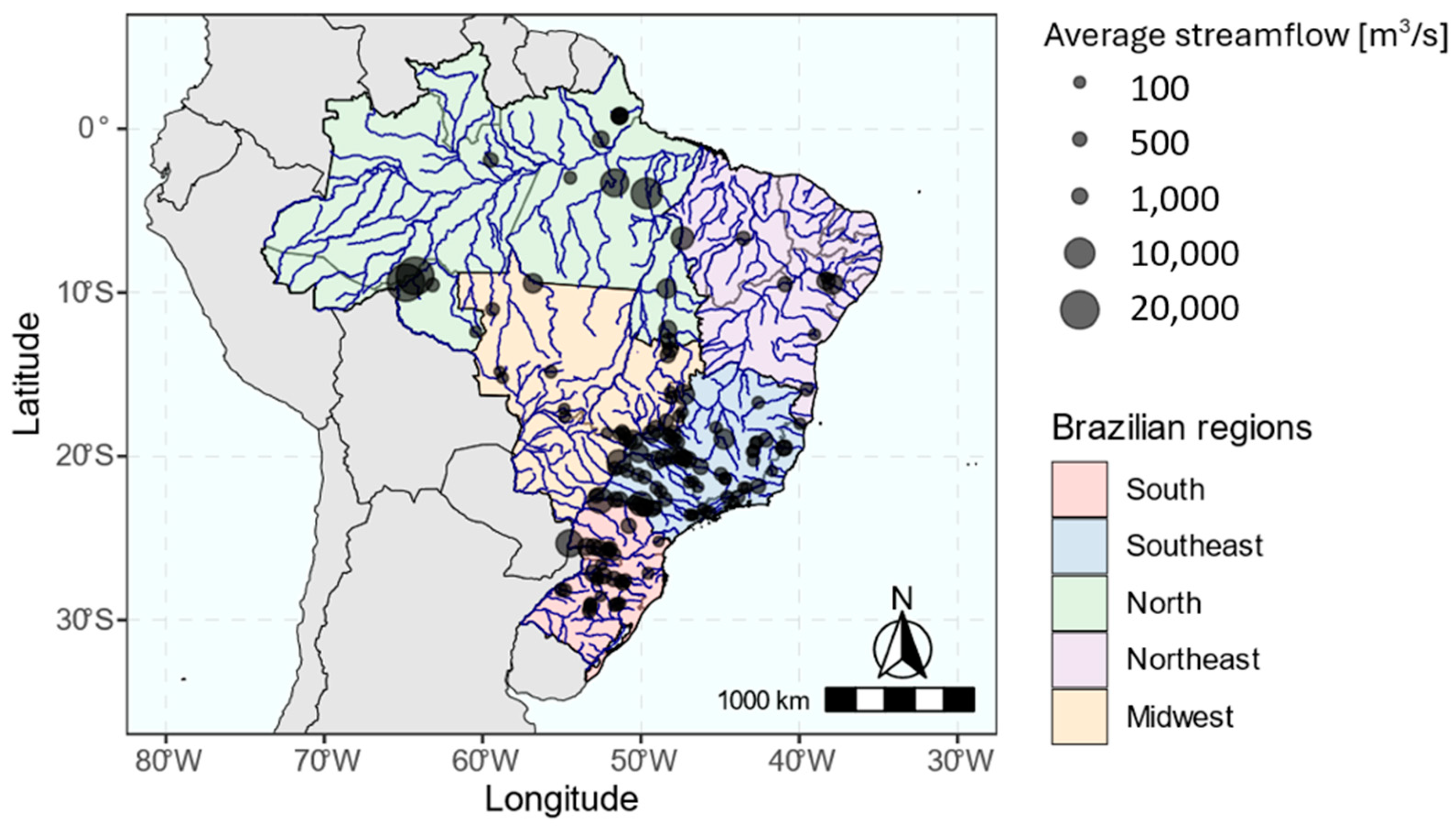
Streamflow rates in Brazilian rivers are tracked by a network of monitoring stations. The collected data are used in a reconstitution process to compute the natural water inflows to each reservoir and hydropower plant, resulting in a set of historical time series of streamflow levels which are later used to feed the streamflow forecasting process. In this study, we employ streamflow time series data from 139 reservoirs and hydropower plants to evaluate the framework shown in Figure 1 and the performance of the individual ensemble members. Figure 3 illustrates the hydro system considered in this study.

3.2. Time Series Forecasting Considerations

In this study, we considered a total of 139 reservoirs and hydropower plants across Brazil. Of these, 67 had their natural inflow rates forecasted using SMAP/ONS, ANNs, and MGB, while the remaining 72 lacked forecasts were made by SMAP/ONS. As a consequence, the backtest evaluation process involved separate assessments for each group.
To produce the backtest simulation forecasts, we employed three rainfall–runoff models: MGB, SMAP/ONS, and ANNs. These models relied on precipitation forecasts for the next 11 days from four different weather forecasting models: ETA40, GEFS, GFS, and ENS. The resulting ensemble of predictions were made by the set of rainfall–runoff models encompasses eight members, GEFS-MGB, inf(GEFS-MGB), median(GEFS-MGB), sup(GEFS-MGB), ETA-MGB, GFS-MGB, SMAP/ONS, and ANNs, all of which underwent a Box–Cox transformation to ensure a normal data distribution prior to the BMA process.
The BMA framework was executed daily and individually for each reservoir and hydropower plant, covering a backtest period of 386 days, from 15 August 2019 to 3 September 2020. BMA weights were updated weekly, specifically on Thursdays, based on the most recent 120 days of measured and predicted streamflows. These updated weights were then normalized and applied to the daily generated ensemble forecasts, resulting in the BMA predictions scenario.

3.3. Overall Performance of BMA and Ensemble Members

3.3.1. The Illustrative Case of Água Vermelha Hydropower Plant

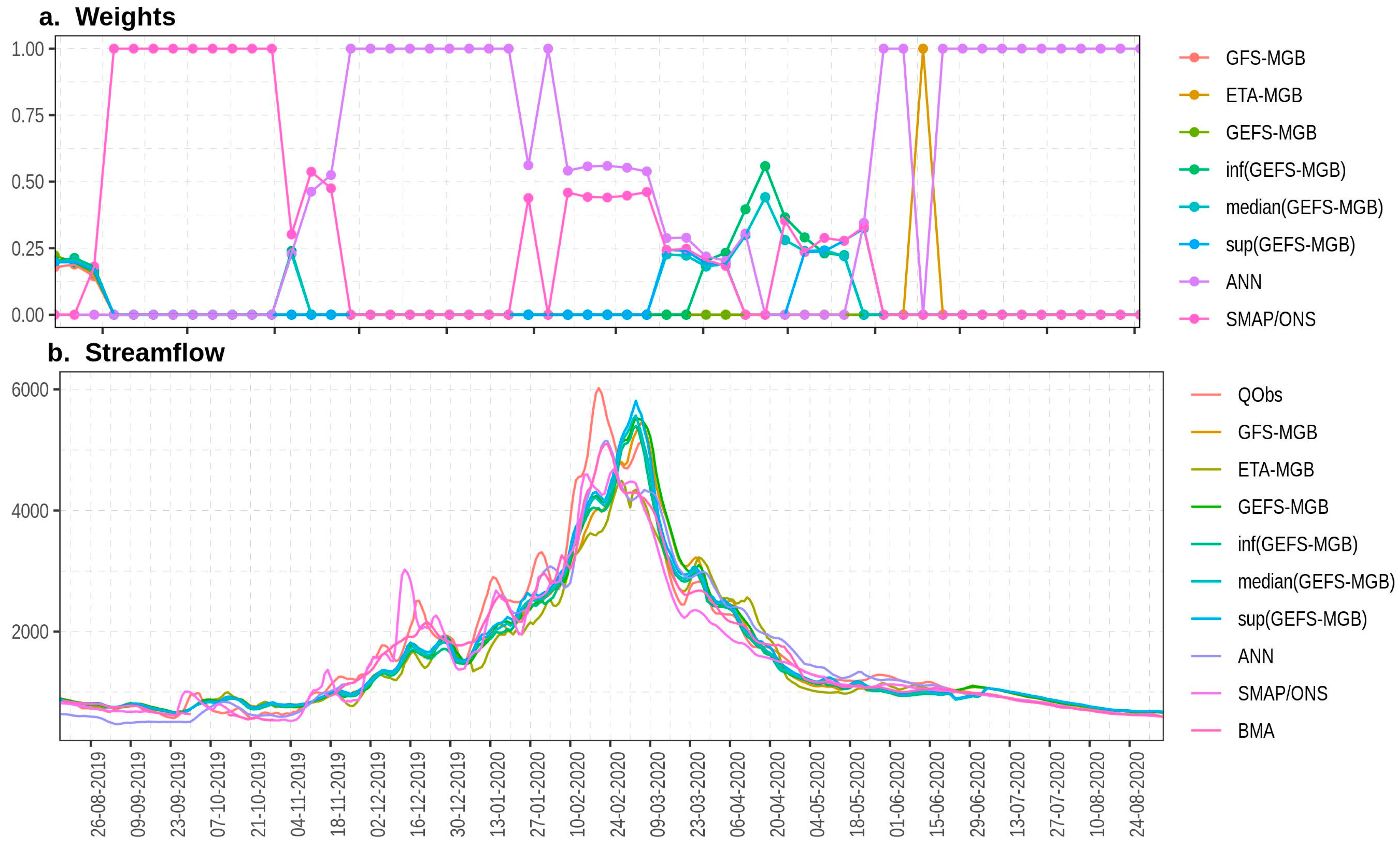
The framework proposed in Figure 1 was tested from August 2019 to September 2020 via backtesting simulations. Over this period, we carried out daily runs, considering a forecast horizon of 11 days ahead for all reservoirs and hydropower plants, as highlighted in Figure 3. For brevity’s sake and considering the large size of the hydro-dominant Brazilian power system, we present the results of the backtesting simulations for all reservoirs and hydropower plants collectively using boxplots and maps. First, however, we illustrate the application of the proposed framework with a single test case to make the process of understanding the methodology easier. Figure 4 shows the BMA predictions, time-variable weights, and streamflow ensemble members related to the Água Vermelha hydropower plant, the last downstream plant in the Grande River basin in the Southeast Brazilian region.
The results for the Água Vermelha hydropower plant indicate that during certain periods (e.g., between August and December 2019), the SMAP/ONS and ANN chains receive greater weighting than other rainfall–runoff chains, revealing that the BMA predictions are not equally affected by the ensemble members. In fact, it is an effect of Occam’s Razor principle that discards ensemble members with low relative performance and strengthens the remaining ones. The selection of ensemble members with good performance can increase the BMA accuracy [101], since the rainfall–runoff chain predictions with poor performance affect the BMA forecasts even when they are low-weighted. As a consequence, the weights that are assigned to the remaining ensemble members (i.e., the ones that are not discarded) become larger, favoring rainfall–runoff chains such as the ANN and SMAP/ONS over MGB-based chains.
Furthermore, note that many ensemble members continue to contribute to the BMA predictions across different periods. Notably, their weights tend to be more similar during certain intervals, such as between February and May 2020. This illustrates that the rainfall–runoff chains have a variable performance that affects the BMA weights, resulting in different weight intensities and model combinations over time. Several factors could be influencing these performance variations, including the potential ineffectiveness of the rainfall–runoff chain in accurately simulating streamflows at certain levels, inconsistencies in the measured streamflow and precipitation data, or possibly, poor precipitation forecasts. In this context, the strategy of applying weekly adjusted weights is designed to capture the changing predictive performance of all rainfall–runoff chains. This is achieved by regularly updating their posterior probability distributions, taking into account the most recent time series of both predicted and observed streamflows. Consequently, this approach helps address the short-term impacts of various sources of uncertainty in the forecasting data.

3.3.2. Case Study Results

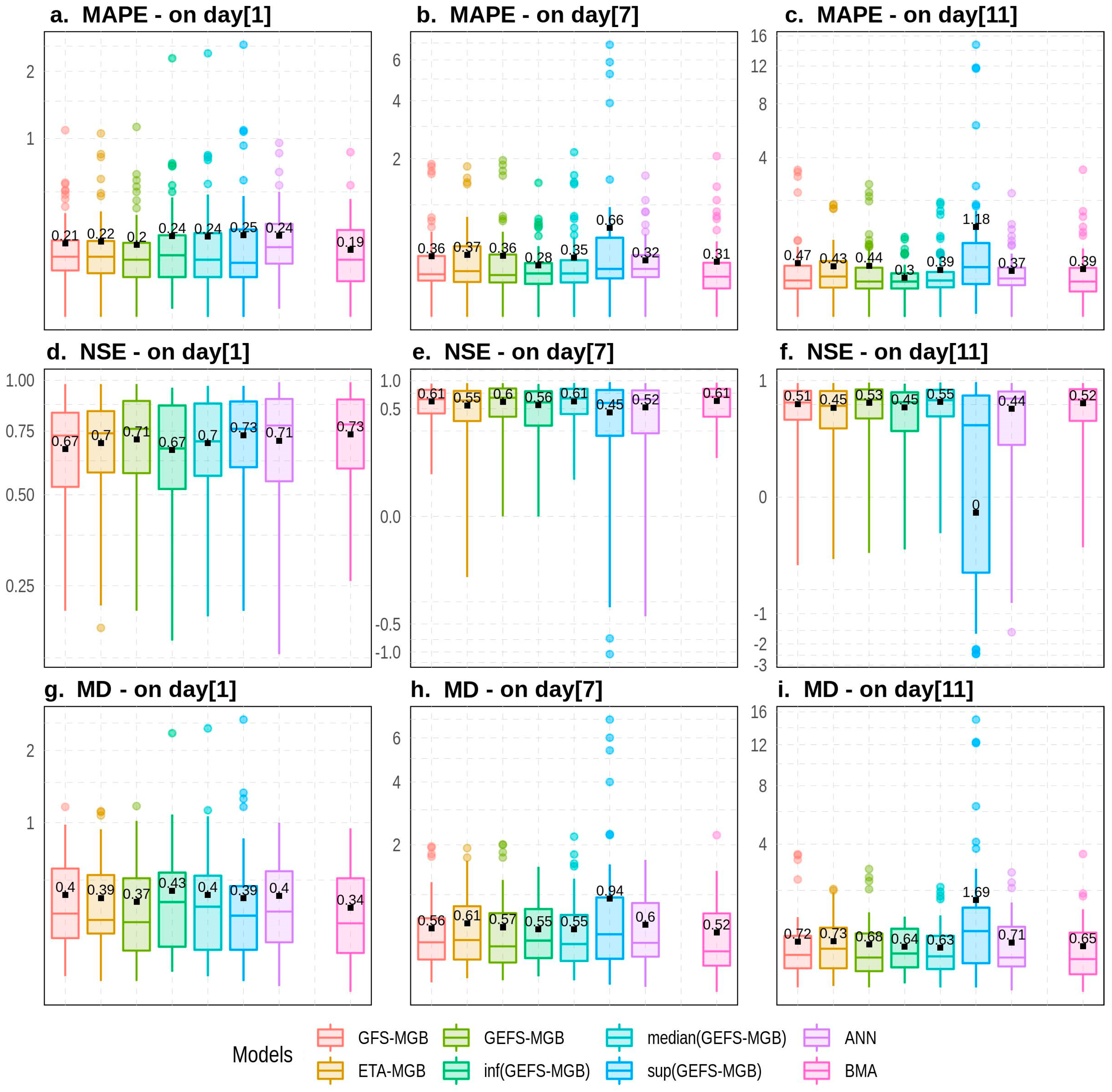
The overall forecasting performance of the rainfall–runoff chains and BMA is illustrated in Figure 5 and Figure A1 in Appendix A using MAPE, NSE, and MD metrics. Figure 5 illustrates the results for 67 reservoirs and hydropower plants, which have their natural inflows simulated by the SMAP/ONS model, primarily located in the South and Southeast regions of Brazil. Conversely, Figure A1 focuses on the remaining 72 reservoirs and hydropower plants, whose natural inflows are not simulated by the SMAP/ONS model and are predominantly situated in the North and Northeast regions of the country. For each reservoir and hydropower plant, these evaluation metrics were calculated individually using datasets from days 1, 7, and 11 of the forecast horizon. The results were then aggregated and presented in the form of boxplots, categorized according to the different rainfall–runoff chains and specific n-day datasets.
Figure 5 indicates that the MGB and ANN models perform similarly on day 1, with an average MAPE ranging from 0.19 to 0.25, suggesting a reasonable accuracy for the initial day of the forecast horizon. For the SMAP/ONS and BMA, the results show superior performance compared to the ANN and MGB-based forecasts, with good accuracy and average MAPEs of 0.16 and 0.15, respectively. However, when evaluating the datasets for days 7 and 11, the performance of BMA and other rainfall–runoff models declines. Generally, all models maintain reasonable accuracy, with the exception of sup(GEFS-MGB), which exhibits poor accuracy and an average MAPE that is greater than 0.5 on day 11, making it the ensemble member with the most significant variation in performance as the forecast horizon extends. When compared to the individual ensemble members, BMA’s predictive accuracy is similar to the best-performing models, with an average MAPE of 0.24 on day 7 and 0.30 on day 11. However, on day 11, it is outperformed by the SMAP/ONS model.
As the length of the forecast horizon increases, uncertainty in precipitation predictions grows [102], potentially accounting for the observed decline in the rainfall–runoff chain’s performance. The SMAP/ONS chain has a significant advantage over other chains, since it incorporates a combination of three precipitation datasets as input. In this chain, predictions from ETA 40, GEFS, and ENS undergo a bias correction process to enhance their estimations of the average rainfall over Brazilian sub-basins. Subsequently, these three sets of post-processed data are combined to obtain a more robust precipitation forecast [103]. Conversely, the MGB, another rainfall–runoff model, is more significantly affected by precipitation data uncertainty for two primary reasons. First, as a distributed model that accounts for the geographical variability of river basins [66], it is inherently sensitive to spatial inaccuracies in rainfall predictions. Second, unlike the SMAP/ONS chain, the precipitation forecasts used in the MGB do not undergo a bias correction process. Therefore, for both the MGB and SMAP/ONS, if the numerical weather forecasting system tends to overestimate or underestimate precipitation, these biased rainfall predictions can adversely impact the performance of the rainfall–runoff chain.
Regarding the efficiency coefficient, BMA has an average NSE of 0.77 and very good efficiency on day 1 (see Table 2 for NSE classification). Most streamflow ensemble members also exhibit satisfactory efficiency, achieving an average NSE of up to 0.63. However, exceptions include sup(GEFS-MGB) and the ANN, both of which display a good level of efficiency. On days 7 and 11, there is a noticeable reduction in the NSE of all ensemble members, with ETA-MGB and sup(GEFS-MGB) experiencing a significant drop in performance. Despite this decline in the efficiency of individual ensemble members, BMA consistently maintains the highest average NSE across all days of the forecast horizon. This underscores the effectiveness of combining models to generate more efficient streamflow predictions. Regarding the distribution of quartiles, the lower limit of boxplots and outliers of all models moves towards the negative region as the n-day increases. This trend indicates that for some reservoirs and hydropower plants, the models have a predictive performance that is worse than the simple average of the measured streamflow values.
The last metric under consideration, the MD, reveals that BMA generally outperforms individual ensemble members in terms of predictive accuracy on days 1, 7, and 11 of the forecast horizon. This result suggests that when the MAPE and NSE are considered together through the MD metric, BMA stands out as the best alternative for forecasting streamflows in the Brazilian South and Southeast regions. Furthermore, in the case of reservoirs and hydroelectric plants in the North and Northeast regions, the results derived from the MAPE, NSE, and MD metrics, as illustrated in Figure A1, are similar to those presented in Figure 5, in which BMA is able to capture the best ensemble members. In summary, Figure A1 shows that according to the MD metric, BMA has the best performance for reservoirs located in the North and Northeast regions on days 1 and 7. These results corroborate the findings of other studies [11,30,32], which also indicate that BMA is capable of generating forecasts that are superior to those of the best ensemble members.
Regarding streamflow forecasting with the BMA approach, it is important to note that the rainfall–runoff model predictions for days 1 through 11 are assigned the same set of weights. Consequently, no distinction is made between the weights applied at the beginning and at the end of the forecast horizon of the same rainfall–runoff chain. This issue is relevant, since some chains had a good performance on day 1 but were unable to maintain the predictive performance when the n-day increases; or even, there are cases in which chains that show average performance on day 1 improved and provided more accurate predictions in the subsequent days. As an example, graphs a., b., and c. from Figure A1 show that inf(GEFS-MGB) did not have the best accuracy on day 1 but was able to outperform the remaining models on days 7 and 11. In order to understand such behavior, it is interesting to assess in future research a BMA approach with weights that differ as the n-day increases. In this case, BMA would be computed using a specific set of weights for each day of the forecast horizon, totaling 11 sets of weights for each reservoir and hydropower plant in SIN.

3.4. Spatial Predictive Performance of BMA

Brazil has large territorial dimensions and lands that make up a significant part of South America. As a result of the Brazilian territorial extension, there is a high diversity of vegetation coverage, land relief, physical and chemical characteristics of soils, land use and occupation, as well as climate conditions [104,105,106], which enable the existence of river basins with different hydrological characteristics. For example, in the Northern Brazilian region, situated within the Amazon rainforest, river basins generate streamflows that are characterized by having a kind of short-term inertia. Meanwhile, in the Southern Brazilian region, where the Atlantic Forest and Pampa biomes predominate, considerable variability in daily streamflows is observed. This high level of short-term variability impacts the streamflow predictability and, consequently, the performance of rainfall–runoff chains. It contributes to the existence of spatial heterogeneity in the BMA model’s predictive performance across the country. For this reason, we investigate the performance of the BMA forecasts for all of Brazil using the MD metric, as illustrated in Figure 6.
The first map, related to day 1, shows that BMA has a high predictive performance and an MD that is lower than 0.3 for several hydropower plants in the North, Northeast, Midwest, and Southeast regions, despite some exceptions along the coast. The Southeast, characterized by a high density of hydropower plants that are essential to guaranteeing adequate energy security levels, stands out due to the predominance of cascade systems with natural inflows that are satisfactorily predicted using the Bayesian approach. In the South, we observe a predominance of hydro reservoirs for which BMA has an inferior predictive performance compared to the ones observed in the remaining regions. Rainfall over this specific region is well distributed throughout the year, and the alternation of wet and dry periods is very fast, contributing to the generation of an unpredictable streamflow regime [107], characterized by high short-term streamflow volatility (e.g., in the Jacuí River, streamflow peaks are often very high when it rains and challenging to predict accurately), which is a typical characteristic of river basins with a short concentration time and a quick streamflow response to precipitation [108]. Such hydrological behavior explains the significant drop in the performance of the Bayesian model, which makes the forecasting process difficult, especially during the rainy season. A similar conclusion can be drawn from the remaining maps, b. and c. We observe the same spatial pattern from map a., but with higher values of the MD, a result that indicates a decreasing predictive performance of the BMA along the forecast horizon.
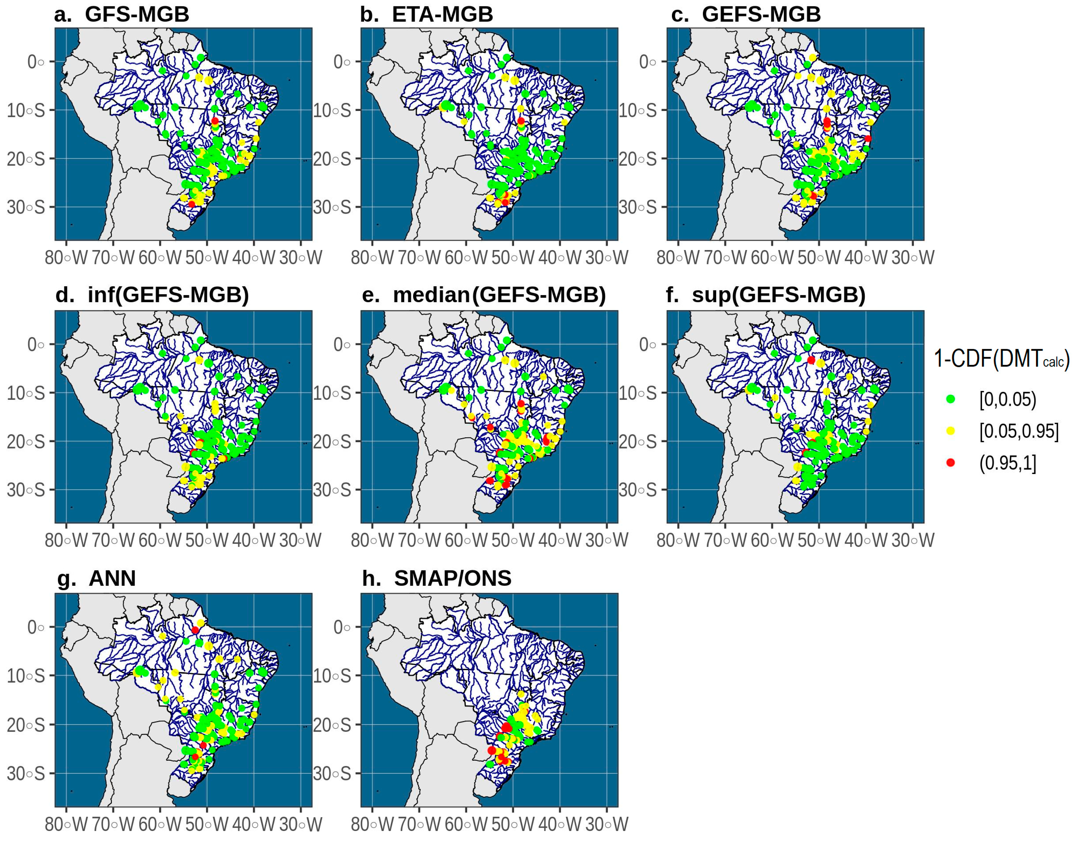
Regarding the predictions from individual rainfall–runoff chains, Figure 7 displays the spatial patterns of the Diebold–Mariano hypothesis test, which is applied to compare the streamflow forecasts from BMA with those of individual ensemble members. In this figure, reservoirs and hydropower plants highlighted in green (or red) are those for which BMA predictions are significantly more (or less) accurate than the ones made by the competing ensemble member. On the other hand, the ones in yellow are those for which there is no statistical difference between predictions from different models. Figure 7 demonstrates that the time series of forecasts performed by GFS-MGB, ETA-MGB, GEFS-MGB, inf(GEFS-MGB), sup(GEFS-MGB), and ANN are significantly less accurate than those made by the BMA in most reservoirs and hydropower plants. In fact, we observe that the number of cases in which the competing ensemble member has an accuracy that is significantly higher than or equal to that of the BMA is quite limited in all regions of Brazil, demonstrating that the predictions that are made according to the Bayesian framework are more consistent and reliable all over the country.
However, in the case of the median(GEFS-MGB) and SMAP/ONS chains, the total number of hydro reservoirs in which the accuracy of the BMA predictions is not significantly different increases, as does the number of cases in which the BMA is outperformed. The results already observed in Figure 5a–c reinforce the outcome of the Diebold–Mariano test regarding the SMAP/ONS chain. The average values of the MAPE on days 1, 7, and 11 for the SMAP/ONS and BMA are very similar, suggesting that BMA can reproduce the accuracy of the best rainfall–runoff chain. In this case, despite the existence of some reservoirs and hydropower plants for which the BMA predictions cannot surpass the competing ensemble member, we notice that when the entire Brazilian hydropower system is taken into account in an assessment based on accuracy measures (and made by the combination of the MAPE and NSE in the DM metric), BMA tends to provide superior predictions.
This result indicates that in a large-scale forecasting problem, the Bayesian approach has advantages that compensate for the cases in which the BMA performs worse than an individual ensemble member. The power of a multi-model ensemble, such as the one that we propose herein, arises from two key factors. First, it benefits from collective offsetting of errors across a range of models. This portfolio approach helps balance out individual model inaccuracies. Second, the ensemble’s strength lies in the consistency of its predictions. These predictions are the result of merging proficient models, each one with unique strengths and weaknesses. Such a combination typically results in predictions that are, on average, more accurate than those made by any single model in the ensemble, as discussed in [109,110].

3.5. Weights Applied to Ensemble Members

As discussed in previous sections, BMA generates a weighted average of forecasts from many model chains. In the approach proposed here, the weights are updated weekly as the time series of forecasted and measured streamflows are updated. This allows BMA to take into account the recent behavior of the rainfall–runoff chains, a relevant feature that needs to be considered when a model’s performance varies over time, as seen during dry, rainy, and transition periods. Furthermore, it is important to recognize that the precise start and end of these periods are not known in advance. Their onset may occur earlier or later compared to previous years. This uncertainty justifies the use of dynamic weighting rather than static weighting for each period.
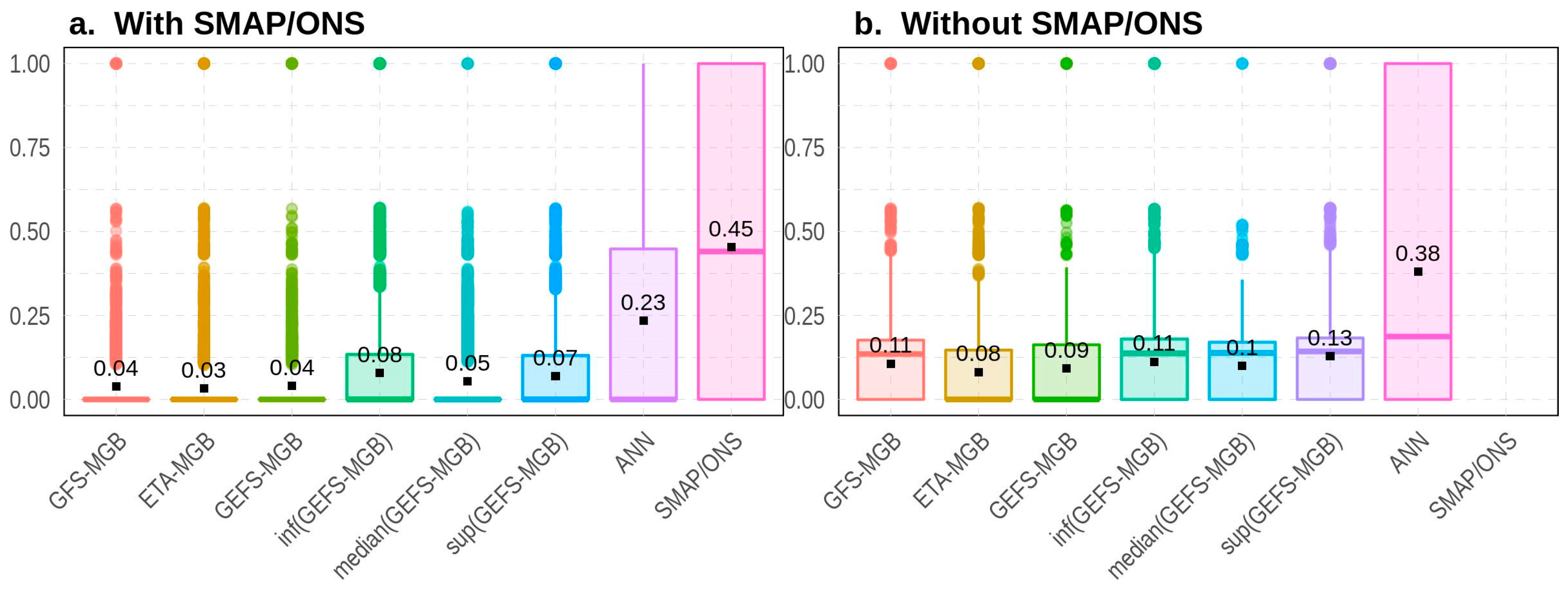
Such evolving behavior impacts the accuracy and efficiency of streamflow forecasts and also affects BMA. This influence is evident in Figure 8, Figure 9 and Figure 10, which display the boxplots of the weights assigned to several rainfall–runoff chains. Figure 8a shows the weights related to 67 hydro reservoirs with natural inflows that are simulated by the SMAP/ONS model without temporal information about when they were computed (i.e., weights computed on different days were grouped by model for a more general evaluation of the results). In this case, the MGB-based chains have weights ranging from 0.03 to 0.08. Their upper limits are also relatively low (below 0.35), with some outliers exceeding 0.5. The similarity in the weights applied to different MGB-based chains, such as GFS-MGB, ETA-MGB, and GEFS-MGB, suggests that without considering the computation time, these chains tend to receive similar weights.
On the other hand, the ANN and SMAP/ONS boxplots indicate that these rainfall–runoff chains have weights with higher values. The ANN has an average weight of 0.23 and an upper limit reaching 1, whereas the SMAP/ONS has an average weight of 0.45, with an upper limit that is also equal to 1. Figure 8a indicates that BMA is mainly influenced by the SMAP/ONS and ANN, while lower weights limit the remaining chains. In contrast, Figure 8b shows that the MGB-based chains have higher average weights than those in Figure 8a, ranging from 0.08 to 0.13. Nevertheless, the ANN model stands out as having the highest weights, with an average weight of 0.38. Our findings indicate that for reservoirs and hydropower plants that are situated in the Southeast and South regions, the SMAP/ONS and ANN chains are the most critical contributors to BMA, while in the case of the North and Northeast regions, the ANN chain stands out.
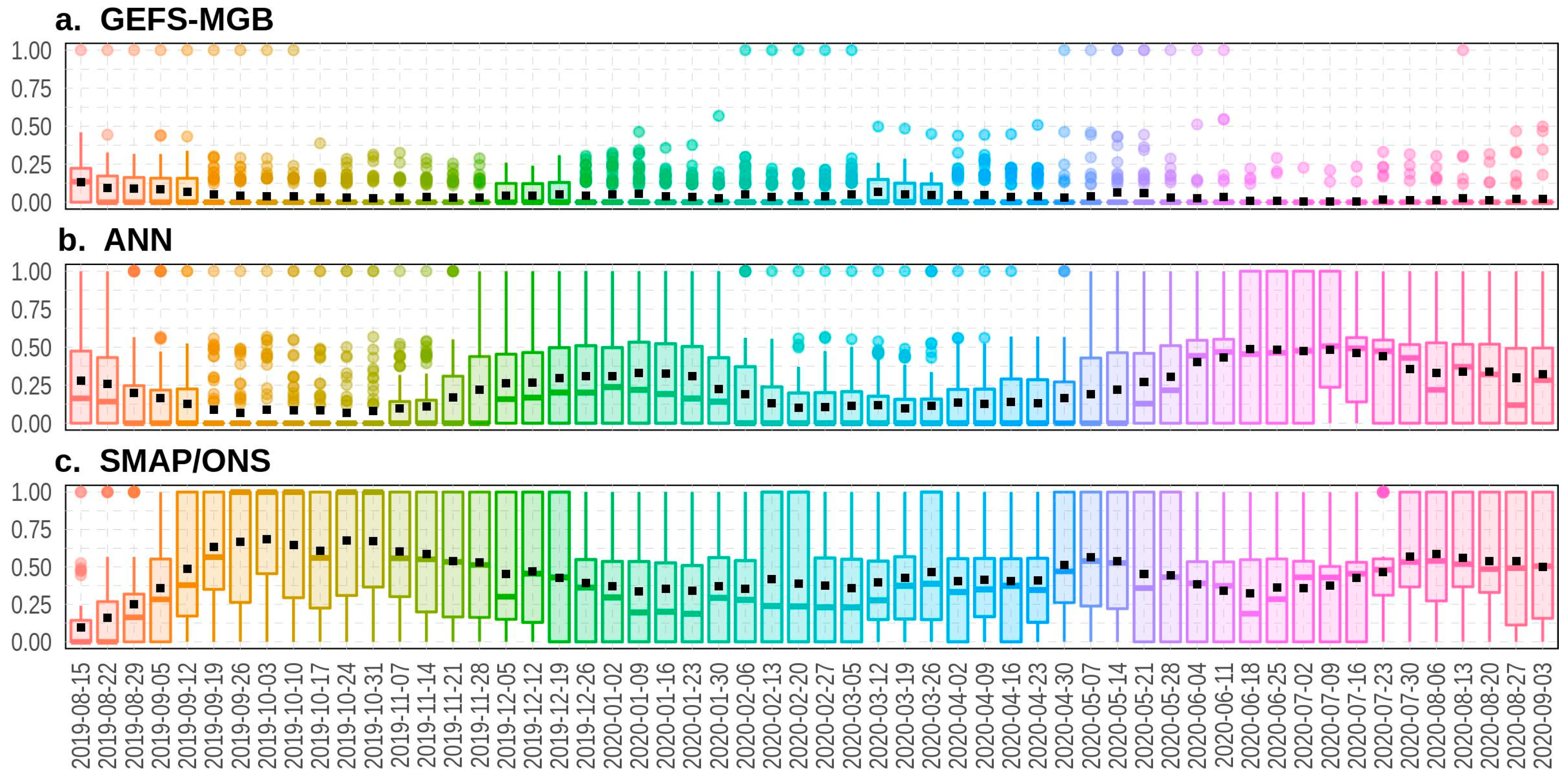
When time is taken into account, weights tend to reflect the recent behavior of the rainfall–runoff chains. As shown in Figure 9, related to hydro reservoirs with inflows that are simulated by the SMAP/ONS, MGB-based chains always present average values of weights that are lower than 0.25. For instance, we observe the case of GEFS-MGB, with average values of weights that are near to zero on several days. In contrast, the ANN and SMAP/ONS display a different pattern. The average values of weights are higher and close to 0.5 in the ANN case but drop to around 0.25 and 0.00 on some days. The SMAP/ONS stands out for having average values of weights that remain close to 0.5 most of the time, reaching 0.75 on some days. Additionally, the complementarity between the weights of the ANN and SMAP/ONS is remarkable. When the average weight of the ANN decreases (or increases), there is a corresponding increase (or decrease) in the average weight of the SMAP/ONS along the time axis.
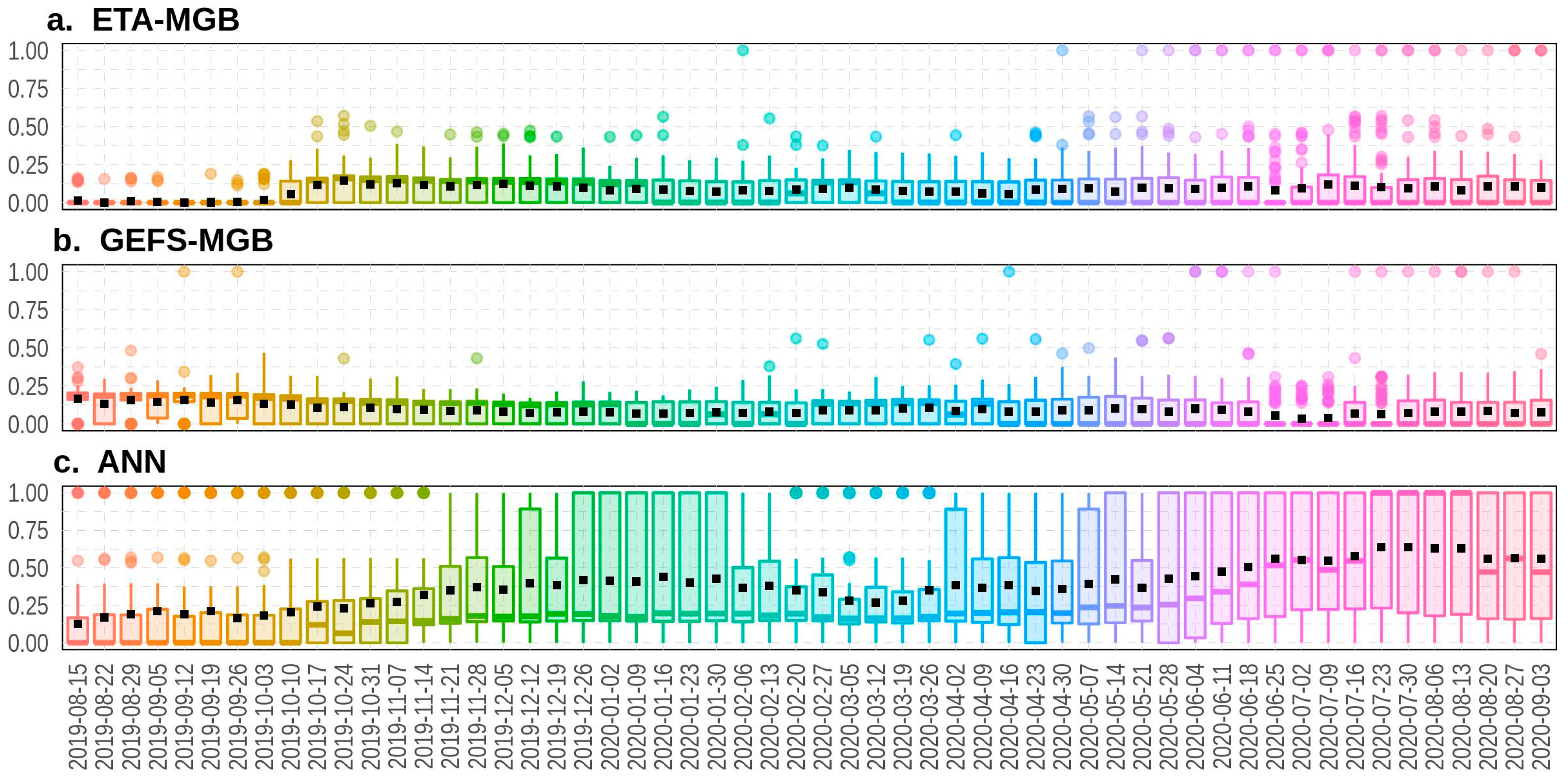
In the case of hydro reservoirs with natural inflows that are not simulated by the SMAP/ONS (refer to Figure 10), the weights assigned to MGB-based chains show a similar pattern to those of ETA-MGB and GEFS-MGB. The average values of weights are slightly higher, and the frequency at which these averages reach zero is low. Meanwhile, the ANN stands out for having high weights along almost the entire time axis, close to 0.75 on many days. Furthermore, it is interesting to note that there is no strong complementarity between the ANN and another specific model.
Throughout the year, we expect the behavior of any rainfall–runoff chain to change during the dry, rainy, and transition periods. This is primarily because making streamflow forecasts becomes more challenging when the rainfall regime is intense and variable. Our approach, which differs from other studies that adopt static weights for each season, circumvents this issue. We use recent data from both measured and forecasted streamflow time series to compute dynamic weights. These weights can be updated daily if necessary, allowing the framework to systematically incorporate new information.

3.6. Remarks and Discussion

The substantive contribution of this research is the development of a multi-model Bayesian framework to enhance streamflow forecasts in hydro-dominant power systems. Designed to serve as an operational tool, it explores Bayesian model averaging to incorporate predictive uncertainty into the forecasting process [27,28,29], enhancing the robustness and reliability of predictions. The proposed method was tested in the Brazilian hydropower system [100], considering a forecast horizon of up to 11 days ahead. The research findings demonstrated that for the Southeast, Midwest, and South regions, BMA produces forecasts with a mean MD ( M A P E 2 + 1 N S E 2 ) [96], which is lower than those obtained for the individual ensemble members on days 1, 7, and 11 (i.e., 0.28, 0.54, and 0.72, see Figure 5), while in the North and Northeast regions, the average MD is lower on days 1 and 7 (i.e., 0.34 and 0.52, see Figure A1). The results of the Diebold–Mariano test [97] also indicated that BMA generates significantly more accurate forecasts than most of the individual ensemble members (i.e., p-value < 0.05, see Figure 7). The only exceptions are the SMAP/ONS and the median(GEFS-MGB), where the number of reservoirs and hydropower plants for which it is not possible to indicate which streamflow forecast is more accurate is large.
The results from the study reveal that, in terms of predictive performance, BMA generally outperforms individual ensemble members at different days of the forecast horizon in the Southeast, Midwest, South, North, and Northeast regions of Brazil. Both the accuracy and the efficiency metrics show that the Bayesian technique produces predictions that are more in line with real streamflows. The rationale for this finding is based on the fact that rainfall–runoff models, differing in structure (such as MGB, the SMAP/ONS, and ANNs) and in the types of input data that they use, like streamflows and forecasted precipitation (for instance, the GFS, GEFS, ETA, and ENS), are effective in detecting intrinsic patterns in the streamflow time series [25,26]. Thus, by integrating models with different strengths and weaknesses, BMA manages to reinforce the positive aspects and mitigate the negatives, resulting in a more reliable forecast [32].
Other studies conducted along the same line of research also indicate that predictions made using Bayesian frameworks are more accurate [11,30,31,32,34]. However, there are methodological differences that must be underscored. In the framework proposed in the current paper, the weights that are applied to the ensemble members are dynamic and updated weekly, taking into account the historical data of observed and forecasted streamflows that are available right up until the forecasting process begins. This process, which updates the posterior probability distribution and adjusts the weights at a higher frequency, ensures that the combined forecasts always incorporate updated information about the performance of the forecasts and the uncertainties that are associated with each ensemble member. Research traditionally limits the ensemble weights to static or unchanging values. Studies developed by other authors, such as those by Duan et al. [32] and Souza Filho et al. [34], while considering different weights for predefined ranges of flows (i.e., for example, very low, low, normal, high, and very high streamflows), maintain invariant values for the weights that are assigned to each range. Approaches like these, based on static datasets for weight computation, do not account for potential variations in model performance over time. Incorporating adaptive mechanisms that adjust weights based on recent data could enhance the robustness and reliability of predictions, ensuring that the model remains responsive to new information and evolving patterns [111]. In our understanding, it is necessary to constantly reassess and adjust weights, with the aim of ensuring the Bayesian framework’s effectiveness in applications extending beyond the academic boundaries.
Another significant aspect of the study, worth highlighting and discussing, is that our framework is able to eliminate the contribution from specific members of the ensemble. As has been emphasized in the paper, while the weights that are assigned to underperforming ensemble members are relatively low in the traditional BMA method, it has been noted that when the number of these underperforming members increases, their collective influence has the potential to compromise the predictive performance of BMA, which underscores the importance of their removal [28,34]. Here, the selection of members that effectively take part in the composition of the BMA is carried out weekly together with the update of weights, following the principle of Occam’s Razor [28] (i.e., models with lower relative performances must be discarded, since they provide predictions that are far less assertive than those provided by the best model). Consequently, the streamflow ensemble’s average is calculated using a subset of models that are supported by the data [29]. In the studies conducted by Duan et al. [32], Wagena et al. [31], and Ajami et al. [11], BMA frameworks were proposed to generate streamflow predictions without discarding ensemble members with low performance. Although these studies indicate that BMA generates more accurate forecasts, it is noteworthy that the ensemble includes members whose weights are significantly lower than those assigned to the top-performing model (members that, if removed, might contribute to improving BMA’s performance).
The dynamism of the proposed Bayesian framework, grounded in the frequent updating of weights and the removal of low-performing members, is a characteristic that makes it suitable for applications aimed at large-scale systems with high hydrological diversity. In hydro-dominant power systems spanning continental dimensions, such as the Brazilian system, watersheds have diverse physical attributes [99,100], resulting in varied hydrological regimes. In some cases, these watersheds generate streamflows that are more difficult to predict due to sharp peaks in flow rates [108]. As a consequence, the predictive performance of some models may vary by area. For instance, a model X that performs well in watershed A may perform poorly in watershed B, thereby proving unsuitable for use in B. Alternatively, this performance pattern may also change over time if, for example, model X starts to underperform in watershed A. The framework that is proposed in this research automatically manages these issues, as it establishes, following the Bayesian theory and using up-to-date data, the ensemble that is believed to be the most suitable for every time series being predicted across spatial and temporal dimensions. This flexibility is a key feature that supports its application in large-scale systems, an advantage not covered by other research in the existing literature [11,30,31,32,34].
The approach proposed here has a variety of advantages. Among the main ones, the following stand out: (a) the framework accounts for the uncertainties in forecasts from rainfall–runoff models (MGB, SMAP/ONS, and ANNs) during the ensemble members’ weighting process, enhancing the robustness of the final forecast; (b) an extensive database is not required for the operationalization of the framework, as the BMA weights are derived from the most recent 120 days of forecast and observed streamflow data, facilitating its application in river basins with newly operational rainfall–runoff models; (c) ensemble members that show low performance are discarded by the principle of Occam’s Razor [28], preventing the degradation of the BMA results; and, additionally, it is worth noting that (d) the weights that are applied in the weighted average are dynamic, which means that they adapt to the signals from the recent history of forecasted and measured streamflows. This feature allows recent changes in performance to be detected and taken into account in the BMA weights.
Despite the outlined advantages, it is important to note that the BMA framework’s reliance on a multi-model ensemble makes its operation more complex compared to a single rainfall–runoff model. Indeed, it is more practical and less costly to operate with a simple structure in which only one mathematical model is used for streamflow forecasting [11]. However, the improvements in accuracy and efficiency of the forecasts that are made by applying BMA justify its use. In electrical power systems with a strong integration of hydropower plants, as is the case in Brazil, streamflow forecasting is a key factor in achieving optimized and robust operation of power plants [13,14], yielding benefits that outweigh the challenges of implementing a more complex framework.

4. Conclusions

This paper addressed the use of Bayesian model averaging to forecast the water inflow in a large-scale hydro-dominant power system. The proposed framework combines streamflow forecasts from several rainfall–runoff chains using weights based on their posterior probability distributions. As a result, better-performing models get higher weights, whereas models with poorer performance receive lower weights, affecting their impact on the ensemble’s average. The approach takes into account the existing limitations of real-time forecasting and incorporates the use of precipitation predictions from weather forecast systems into rainfall–runoff modeling. The limited availability of historical forecasts and the need to capture the recent performance of rainfall–runoff chains lead to the use of dynamic ensemble weights, which are updated weekly, avoiding the need for a very long time series to operationalize the framework. Regarding the data from the numerical weather forecasting models, it should be noted that the forecasted precipitation introduces significant uncertainties in streamflow forecasts. However, this effect is taken into account in the model combination process, when historical time series from rainfall–runoff models are used in the computation of real-time weights.
The results have shown that the proposed approach is more robust than using a single rainfall–runoff chain, since we consider the uncertainty of each ensemble member. In general, a rainfall–runoff chain that performs well in a specific river basin may have medium or lower predictive performance in another river basin. The proposed framework takes advantage of this and gives more value to the forecasts of the best rainfall–runoff chains of each river basin (also considering each reservoir and hydropower plant individually), resulting in an average MD ( M A P E 2 + 1 N S E 2 ) that is better than the ones computed for the individual ensemble members.
Future work should focus on improving the model averaging process by applying a different set of weights to each day of the forecast horizon. In this study, we demonstrated that the predictive performance of rainfall–runoff chains changes over time. Consequently, we believe that if the weights are able to capture such a characteristic, they are likely to reduce the degradation of streamflow predictions as the n-day of the forecast horizon increases. Additionally, training different architectures of artificial neural networks (such as long short-term memory, Bayesian networks, and transformers) along with machine learning models (like support vector machines, random forests, and Ridge regression) should be considered for inclusion in the framework and BMA forecasts.

Author Contributions

Conceptualization, all authors; methodology, F.L.R.T., L.M.M.L. and M.S.R.; software, F.L.R.T.; validation, L.M.M.L., M.S.R. and A.R.d.Q.; formal analysis, all authors; resources, F.L.R.T., L.M.M.L. and M.S.R.; writing—original draft preparation, F.L.R.T.; writing—review and editing, all authors; project administration, J.W.M.L.; funding acquisition, J.W.M.L. All authors have read and agreed to the published version of the manuscript.

Funding

The authors would like to thank CNPQ and Energisa for funding and supporting the activities developed under the Research and Development Project “Neural networks applied to forecasting inflow and demand to support the formation of electricity prices in the short term”, R&D PD-06585-RT-01.

Data Availability Statement

Data are available from the authors by request.

Conflicts of Interest

The authors declare no conflicts of interest.

Appendix A

Figure A1. MAPE, NSE, and MD computed using natural inflows to reservoirs and hydropower plants not simulated by SMAP/ONS. Datasets from backtesting simulation were used to evaluate the streamflow forecasts of 72 reservoir and hydropower plants. Black squares represent the average values in each boxplot, and the colored dots represent the outliers.
Water 16 00586 g0a1

References

  1. Tundisi, J.G. Water Resources in the Future: Problems and Solutions. Estud. Avançados 2008, 22, 7–16. [Google Scholar] [CrossRef]
  2. Cheng, M.; Fang, F.; Kinouchi, T.; Navon, I.M.; Pain, C.C. Long Lead-Time Daily and Monthly Streamflow Forecasting Using Machine Learning Methods. J. Hydrol. 2020, 590, 125376. [Google Scholar] [CrossRef]
  3. Schmitt Quedi, E.; Mainardi Fan, F. Sub Seasonal Streamflow Forecast Assessment at Large-Scale Basins. J. Hydrol. 2020, 584, 124635. [Google Scholar] [CrossRef]
  4. Sohrabi, S.; Brissette, F.P.; Arsenault, R. Coupling Large-Scale Climate Indices with a Stochastic Weather Generator to Improve Long-Term Streamflow Forecasts in a Canadian Watershed. J. Hydrol. 2020, 594, 125925. [Google Scholar] [CrossRef]
  5. Silva, F.d.N.R.d.; Alves, J.L.D.; Cataldi, M. Climate Downscaling over South America for 1971–2000: Application in SMAP Rainfall-Runoff Model for Grande River Basin. Clim. Dyn. 2019, 52, 681–696. [Google Scholar] [CrossRef]
  6. Cloke, H.L.; Pappenberger, F. Ensemble Flood Forecasting: A Review. J. Hydrol. 2009, 375, 613–626. [Google Scholar] [CrossRef]
  7. Moges, E.; Demissie, Y.; Larsen, L.; Yassin, F. Review: Sources of Hydrological Model Uncertainties and Advances in Their Analysis. Water 2021, 13, 28. [Google Scholar] [CrossRef]
  8. Draper, D. Assessment and Propagation of Model Uncertainty. J. R. Stat. Soc. 1995, 57, 45–97. [Google Scholar] [CrossRef]
  9. Bourdin, D.R.; Stull, R.B. Bias-Corrected Short-Range Member-to-Member Ensemble Forecasts of Reservoir Inflow. J. Hydrol. 2013, 502, 77–88. [Google Scholar] [CrossRef]
  10. Zahmatkesh, Z.; Karamouz, M.; Nazif, S. Uncertainty Based Modeling of Rainfall-Runoff: Combined Differential Evolution Adaptive Metropolis (DREAM) and K-Means Clustering. Adv. Water Resour. 2015, 83, 405–420. [Google Scholar] [CrossRef]
  11. Ajami, N.K.; Duan, Q.; Sorooshian, S. An Integrated Hydrologic Bayesian Multimodel Combination Framework: Confronting Input, Parameter, and Model Structural Uncertainty in Hydrologic Prediction. Water Resour. Res. 2007, 43, 1–19. [Google Scholar] [CrossRef]
  12. Stergiadi, M.; Di Marco, N.; Avesani, D.; Righetti, M.; Borga, M. Impact of Geology on Seasonal Hydrological Predictability in Alpine Regions by a Sensitivity Analysis Framework. Water 2020, 12, 2255. [Google Scholar] [CrossRef]
  13. Galletti, A.; Avesani, D.; Bellin, A.; Majone, B. Detailed Simulation of Storage Hydropower Systems in Large Alpine Watersheds. J. Hydrol. 2021, 603, 127125. [Google Scholar] [CrossRef]
  14. Smajgl, A.; Ward, J.; Pluschke, L. The Water-Food-Energy Nexus—Realising a New Paradigm. J. Hydrol. 2016, 533, 533–540. [Google Scholar] [CrossRef]
  15. Bahramian, K.; Nathan, R.; Western, A.W.; Ryu, D. Towards an Ensemble-Based Short-Term Flood Forecasting Using an Event-Based Flood Model-Incorporating Catchment-Average Estimates of Soil Moisture. J. Hydrol. 2021, 593, 125828. [Google Scholar] [CrossRef]
  16. Brito, B.O.; Salgado, R.M.; Beijo, L.A. Intelligent Modeling for Streamflow Forecasting. IEEE Lat. Am. Trans. 2016, 14, 3669–3677. [Google Scholar] [CrossRef]
  17. Siqueira, V.A.; Fan, F.M.; de Paiva, R.C.D.; Ramos, M.H.; Collischonn, W. Potential Skill of Continental-Scale, Medium-Range Ensemble Streamflow Forecasts for Flood Prediction in South America. J. Hydrol. 2020, 590, 125430. [Google Scholar] [CrossRef]
  18. Ribeiro, V.H.A.; Reynoso-Meza, G.; Siqueira, H.V. Multi-Objective Ensembles of Echo State Networks and Extreme Learning Machines for Streamflow Series Forecasting. Eng. Appl. Artif. Intell. 2020, 95, 103910. [Google Scholar] [CrossRef]
  19. Sabzipour, B.; Arsenault, R.; Brissette, F. Evaluation of the Potential of Using Subsets of Historical Climatological Data for Ensemble Streamflow Prediction (ESP) Forecasting. J. Hydrol. 2020, 595, 125656. [Google Scholar] [CrossRef]
  20. Jeong, D., Il; Kim, Y.O. Rainfall-Runoff Models Using Artificial Neural Networks for Ensemble Streamflow Prediction. Hydrol. Process. 2005, 19, 3819–3835. [Google Scholar] [CrossRef]
  21. Kasiviswanathan, K.S.; Cibin, R.; Sudheer, K.P.; Chaubey, I. Constructing Prediction Interval for Artificial Neural Network Rainfall-Runoff Models Based on Ensemble Simulations. J. Hydrol. 2013, 499, 275–288. [Google Scholar] [CrossRef]
  22. Saraiva, S.V.; Carvalho, F.d.O.; Santos, C.A.G.; Barreto, L.C.; de Macedo Machado Freire, P.K. Daily Streamflow Forecasting in Sobradinho Reservoir Using Machine Learning Models Coupled with Wavelet Transform and Bootstrapping. Appl. Soft Comput. 2021, 102, 107081. [Google Scholar] [CrossRef]
  23. Shamseldin, A.Y.; O’Connor, K.M.; Liang, G.C. Methods for Combining the Outputs of Different Rainfall-Runoff Models. J. Hydrol. 1997, 197, 203–229. [Google Scholar] [CrossRef]
  24. Kim, Y.-O.; Jeong, D.; Ko, I.H. Combining Rainfall-Runoff Model Outputs for Improving Ensemble Streamflow Prediction. J. Hydrol. Eng. 2006, 11, 578–588. [Google Scholar] [CrossRef]
  25. Devineni, N.; Sankarasubramanian, A.; Ghosh, S. Multimodel Ensembles of Streamflow Forecasts: Role of Predictor State in Developing Optimal Combinations. Water Resour. Res. 2008, 44, W09404. [Google Scholar] [CrossRef]
  26. Muhammad, A.; Stadnyk, T.A.; Unduche, F.; Coulibaly, P. Multi-Model Approaches for Improving Seasonal Ensemble Streamflow Prediction Scheme with Various Statistical Post-Processing Techniques in the Canadian Prairie Region. Water 2018, 10, 1604. [Google Scholar] [CrossRef]
  27. Fragoso, T.M.; Bertoli, W.; Louzada, F. Bayesian Model Averaging: A Systematic Review and Conceptual Classification. Int. Stat. Rev. 2018, 86, 1–28. [Google Scholar] [CrossRef]
  28. Raftery, A.E.; Madigan, D.; Hoeting, J.A. Bayesian Model Averaging for Linear Regression Models. J. Am. Stat. Assoc. 1997, 92, 179–191. [Google Scholar] [CrossRef]
  29. Hoeting, J.A.; Madigan, D.; Raftery, A.E.; Volinsky, C.T. Bayesian Model Averaging: A Tutorial. Stat. Sci. 1999, 14, 382–401. [Google Scholar] [CrossRef]
  30. He, S.; Guo, S.; Liu, Z.; Yin, J.; Chen, K.; Wu, X. Uncertainty Analysis of Hydrological Multi-Model Ensembles Based on CBP-BMA Method. Hydrol. Res. 2018, 49, 1636–1651. [Google Scholar] [CrossRef]
  31. Wagena, M.B.; Goering, D.; Collick, A.S.; Bock, E.; Fuka, D.R.; Buda, A.; Easton, Z.M. Comparison of Short-Term Streamflow Forecasting Using Stochastic Time Series, Neural Networks, Process-Based, and Bayesian Models. Environ. Model. Softw. 2020, 126, 104669. [Google Scholar] [CrossRef]
  32. Duan, Q.; Ajami, N.K.; Gao, X.; Sorooshian, S. Multi-Model Ensemble Hydrologic Prediction Using Bayesian Model Averaging. Adv. Water Resour. 2007, 30, 1371–1386. [Google Scholar] [CrossRef]
  33. See, L.; Openshaw, S. A Hybrid Multi-Model Approach to River Level Forecasting. Hydrol. Sci. J. 2000, 45, 523–536. [Google Scholar] [CrossRef]
  34. Souza Filho, F.d.A.d.; Rocha, R.V.; Estácio, Á.B.; Rolim, L.Z.R.; Pontes Filho, J.D.d.A.; Porto, V.C.; Guimarães, S.O. Enhancing Streamflow Forecasting for the Brazilian Electricity Sector: A Strategy Based on a Hyper-Multimodel. Braz. J. Water Resour. 2023, 28, e45. [Google Scholar] [CrossRef]
  35. Box, G.E.P.; Draper, N.R. Empirical Model-Building and Response Surfaces; John Wiley & Sons, Inc.: Hoboken, NJ, USA, 1987; Volume 37, ISBN 9780471810339. [Google Scholar]
  36. Kimura, R. Numerical Weather Prediction. J. Wind Eng. Ind. Aerodyn. 2002, 90, 1403–1414. [Google Scholar] [CrossRef]
  37. Kanamitsu, M.; Alpert, J.C.; Campana, K.A.; Caplan, P.M.; Deaven, D.G.; Iredell, M.; Katz, B.; Pan, H.-L.; Sela, J.; White, G.H. Recent Changes Implemented into the Global Forecast System at NMC. Weather. Forecast. 1991, 6, 425–435. [Google Scholar] [CrossRef]
  38. EMC. Global Forecast System. Available online: https://www.emc.ncep.noaa.gov/emc/pages/numerical_forecast_systems/gfs.php (accessed on 22 November 2023).
  39. Lien, G.Y.; Kalnay, E.; Miyoshi, T.; Huffman, G.J. Statistical Properties of Global Precipitation in the NCEP GFS Model and TMPA Observations for Data Assimilation. Mon. Weather Rev. 2016, 144, 663–679. [Google Scholar] [CrossRef]
  40. NCEI. Global Forecast System. Available online: https://www.ncei.noaa.gov/products/weather-climate-models/global-forecast#:~:text=The%20Global%20Forecast%20System%20(GFS,moisture%2C%20and%20atmospheric%20ozone%20concentration (accessed on 14 August 2023).
  41. NCEP. GFS Dataset. Available online: https://ftp.ncep.noaa.gov/data/nccf/com/gfs/prod/ (accessed on 21 May 2023).
  42. NCEI. Global Ensemble Forecast System. Available online: https://www.ncei.noaa.gov/products/weather-climate-models/global-ensemble-forecast (accessed on 21 September 2023).
  43. Zhou, X.; Zhu, Y.; Hou, D.; Luo, Y.; Peng, J.; Wobus, R. Performance of the New NCEP Global Ensemble Forecast System in a Parallel Experiment. Weather Forecast 2017, 32, 1989–2004. [Google Scholar] [CrossRef]
  44. NCEP. GEFS Dataset. Available online: https://ftp.ncep.noaa.gov/data/nccf/com/gens/prod/ (accessed on 21 May 2023).
  45. Chou, S.C. Regional ETA Model. Climanálise 1996, 1, 203–207. [Google Scholar]
  46. Mesinger, F. A Blocking Technique for Representation of Mountains in Atmospheric Models. Riv. Meteorol. Aeronaut. 1984, 44, 195–202. [Google Scholar]
  47. Moreto, V.B.; Rolim, G.d.S.; Esteves, J.T.; Vanuytrecht, E.; Chou, S.C. Sugarcane Decision-Making Support Using Eta Model Precipitation Forecasts. Meteorol. Atmos. Phys. 2021, 133, 181–191. [Google Scholar] [CrossRef]
  48. ONS. ETA Model Dataset. Available online: https://sintegre.ons.org.br/sites/9/38/paginas/produtos-dinamicos/meteorologia.aspx (accessed on 21 April 2023).
  49. ECMWF. ENS—Ensemble Forecasts. Available online: https://confluence.ecmwf.int/display/FUG/ENS+-+Ensemble+Forecasts (accessed on 19 April 2023).
  50. ECMWF. The ECMWF Integrated Forecasting System. Available online: https://confluence.ecmwf.int/display/FUG/2+The+ECMWF+Integrated+Forecasting+System+-+IFS (accessed on 2 April 2023).
  51. ONS. ENS Dataset. Available online: https://sintegre.ons.org.br/sites/9/38/paginas/produtos-dinamicos/meteorologia.aspx (accessed on 21 April 2023).
  52. ONS. Update of the Historical Streamflow Time Series—Period from 1931 to 2019; REL 142/2020; ONS: Rio de Janeiro, RJ, Brazil, 2020.
  53. ONS. Historical Time Series of Daily Natural Streamflows Dataset. Available online: https://sintegre.ons.org.br/sites/9/13/84 (accessed on 2 March 2023).
  54. ONS. Methodology for Reconstitution and Treatment of Natural Streamflows; NT 144/2018; ONS: Rio de Janeiro, RJ, Brazil, 2018.
  55. ONS. Hydraulic-Hydrological Reports. Available online: https://sintegre.ons.org.br/sites/9/13/56/paginas/servicos/produtos.aspx (accessed on 2 March 2023).
  56. Da Silva, B.C.; Tucci, C.E.M.; Collischonn, W. Streamflow Forecast with Hydroclimatic Models. Braz. J. Water Resour. 2006, 11, 15–29. [Google Scholar] [CrossRef]
  57. Eslamian, S. Handbook of Engineering Hydrology: Modeling, Climate Change, and Variability; Eslamian, S., Ed.; CRS Press: Boca Ratom, FL, USA, 2014; ISBN 9781466552463. [Google Scholar]
  58. Sitterson, J.; Knightes, C.; Parmar, R.; Wolfe, K.; Muche, M.; Avant, B. An Overview of Rainfall-Runoff Model Types; EPA/600/R-14/152; Environmental Protection Agency: Athens, GA, USA, 2017. [Google Scholar]
  59. Niu, W.; Feng, Z. Evaluating the Performances of Several Artificial Intelligence Methods in Forecasting Daily Streamflow Time Series for Sustainable Water Resources Management. Sustain. Cities Soc. 2021, 64, 102562. [Google Scholar] [CrossRef]
  60. De Faria, V.A.D.; de Queiroz, A.R.; Lima, L.M.; Lima, J.W.M.; da Silva, B.C. An Assessment of Multi-Layer Perceptron Networks for Streamflow Forecasting in Large-Scale Interconnected Hydrosystems. Int. J. Environ. Sci. Technol. 2021, 19, 5819–5838. [Google Scholar] [CrossRef]
  61. Rasmussen, P.F.; Salas, J.D.; Fagherazzi, L.; Rassam, J.-C.; Bobée, B. Estimation and Validation of Contemporaneous PARMA Models for Streamflow Simulation. Water Resour. Res. 1996, 32, 3151–3160. [Google Scholar] [CrossRef]
  62. Tongal, H.; Booij, M.J. Simulation and Forecasting of Streamflows Using Machine Learning Models Coupled with Base Flow Separation. J. Hydrol. 2018, 564, 266–282. [Google Scholar] [CrossRef]
  63. Yu, X.; Wang, Y.; Wu, L.; Chen, G.; Wang, L.; Qin, H. Comparison of Support Vector Regression and Extreme Gradient Boosting for Decomposition-Based Data-Driven 10-Day Streamflow Forecasting. J. Hydrol. 2020, 582, 124293. [Google Scholar] [CrossRef]
  64. Liu, Z.; Zhou, P.; Chen, G.; Guo, L. Evaluating a Coupled Discrete Wavelet Transform and Support Vector Regression for Daily and Monthly Streamflow Forecasting. J. Hydrol. 2014, 519, 2822–2831. [Google Scholar] [CrossRef]
  65. Lopes, J.E.G.; Braga, B.P.F.; Conejo, J.G.L. SMAP: A Simplified Hydrologic Model. In Applied Modeling in Catchment Hydrology; Singh, V.P., Ed.; Water Resources Publications: Littleton, CO, USA, 1982; pp. 167–176. ISBN 1887201963. [Google Scholar]
  66. Collischonn, W.; Allasia, D.; da Silva, B.C.; Tucci, C.E.M. The MGB-IPH Model for Large-Scale Rainfall-Runoff Modelling. Hydrol. Sci. J. 2007, 52, 878–895. [Google Scholar] [CrossRef]
  67. Collischonn, W.; Tucci, C.E.M. Hydrological Simulation of Large Basins. Braz. J. Water Resour. 2001, 6, 95–118. [Google Scholar] [CrossRef]
  68. Beven, K.J. 122: Rainfall-Runoff Modeling: Introduction. In Encyclopedia of Hydrological Sciences; Anderson, M.G., Ed.; John Wiley & Sons: Hoboken, NJ, USA, 2005; pp. 1–12. [Google Scholar]
  69. De Queiroz, A.R.; Marangon Lima, L.M.; Marangon Lima, J.W.; Da Silva, B.C.; Scianni, L.A. Climate Change Impacts in the Energy Supply of the Brazilian Hydro-Dominant Power System. Renew. Energy 2016, 99, 379–389. [Google Scholar] [CrossRef]
  70. De Queiroz, A.R.; Faria, V.A.D.; Lima, L.M.M.; Lima, J.W.M. Hydropower Revenues under the Threat of Climate Change in Brazil. Renew. Energy 2019, 133, 873–882. [Google Scholar] [CrossRef]
  71. Kuki, C.A.C.; Torres, F.L.R.; de Faria, V.A.D.; de Queiroz, A.R.; Lima, L.M.M.; Lima, J.W.M. Short-Term Streamflow Forecast Strategies: A Case Study in the Grande and Paranaíba River Basins. In Proceedings of the Anais do XXIII Congresso Brasileiro de Automática, Virtual Event, 23–26 November 2020; Sociedade Brasileira de Automática: Campinas, SP, Brazil, 2020; pp. 1–8. [Google Scholar]
  72. Kuki, C.A.C. Methodology for Forecasting Energy Prices Considering Streamflow Uncertainties. Master’s Thesis, Institute of Electrical Systems of Energy, Federal University of Itajubá, Itajubá, MG, Brazil, 2020. [Google Scholar]
  73. Da Silva, B.C.; Collischonn, W.; Tucci, C.E.M.; Clarke, R.T.; Corbo, M.D. Short-Term Hydroclimatic Streamflow Forecasting in the São Francisco River Basin. Braz. J. Water Resour. 2007, 12, 21–41. [Google Scholar] [CrossRef]
  74. Collischonn, W.; Gama, C.H.A.; Siqueira, V.A.; Paiva, R.C.D.; Fleischmann, A.S. MGB Reference Manual 2020; IPH: Porto Alegre, RS, Brazil, 2020. [Google Scholar]
  75. Kuki, C.A.C.; Torres, F.L.R.; de Faria, V.A.D.; de Queiroz, A.R.; Lima, L.M.M.; Lima, J.W.M. Streamflow Forecasting Strategy for Short-Term Electricity Price Formation. In Proceedings of the Anais do LII Simpósio Brasileiro de Pesquisa Operacional; Galoá: João Pessoa, PB, Brazil, 2020; pp. 1–12. [Google Scholar]
  76. Maciel, G.M.; Cabral, V.A.; Marcato, A.L.M.; Júnior, I.C.S.; Honório, L.D.M. Daily Water Flow Forecasting via Coupling between SMAP and Deep Learning. IEEE Access 2020, 8, 204660–204675. [Google Scholar] [CrossRef]
  77. De Paiva, L.F.G.; Montenegro, S.M.; Cataldi, M. Prediction of Monthly Flows for Três Marias Reservoir (São Francisco River Basin) Using the CFS Climate Forecast Model. Braz. J. Water Resour. 2020, 25, 1–18. [Google Scholar] [CrossRef]
  78. Nunes, F.M.S.; de Farias, C.A.S.; Martins, W.A.; Almeida, R.N.; Leite, J.C.A. Hydrological Modelling Using SMAP for Estimating Monthly Streamflows in Piancó River Basin. Rev. Verde De Agroecol. E Desenvolv. Sustentável 2014, 9, 289–295. [Google Scholar]
  79. Cavalcante, M.R.G.; da Cunha Luz Barcellos, P.; Cataldi, M. Flash Flood in the Mountainous Region of Rio de Janeiro State (Brazil) in 2011: Part I—Calibration Watershed through Hydrological SMAP Model. Nat. Hazards 2020, 102, 1117–1134. [Google Scholar] [CrossRef]
  80. ONS. Application of the SMAP/ONS Model to Forecast Streamflows within the Scope of the SIN; NT 97/2018-RV4; ONS: Rio de Janeiro, RJ, Brazil, 2020.
  81. ONS. Application of the SMAP/ONS Model to Forecast Streamflows within the Scope of the SIN; ONS 97/2018-RV7; ONS: Rio de Janeiro, RJ, Brazil, 2018.
  82. ONS. SMAP Data. Available online: https://sintegre.ons.org.br/sites/9/13/82/paginas/servicos/produtos.aspx (accessed on 21 April 2023).
  83. McCulloch, W.S.; Pitts, W.H. A Logical Calculus of the Ideas Immanent in Nervous Activity. Bull. Math. Biophys. 1943, 5, 115–133. [Google Scholar] [CrossRef]
  84. Rosenblatt, F. The Perceptron: A Probabilistic Model for Information Storage and Organization in the Brain. Psychol. Rev. 1958, 65, 386–408. [Google Scholar] [CrossRef]
  85. Rumelhart, D.E.; Hinton, G.E.; Williams, R.J. Learning Representations by Back-Propagating Errors. Nature 1986, 323, 533–536. [Google Scholar] [CrossRef]
  86. Krogh, A. What Are Artificial Neural Networks? Nat. Biotechnol. 2008, 26, 195–197. [Google Scholar] [CrossRef]
  87. Hinne, M.; Gronau, Q.F.; van den Bergh, D.; Wagenmakers, E.-J. A Conceptual Introduction to Bayesian Model Averaging. Adv. Methods Pract. Psychol. Sci. 2020, 3, 200–215. [Google Scholar] [CrossRef]
  88. Wasserman, L. Bayesian Model Selection and Model Averaging. J. Math. Psychol. 2000, 44, 92–107. [Google Scholar] [CrossRef]
  89. Moon, T.K. The Expectation-Maximization Algorithm. IEEE Signal Process. Mag. 1996, 13, 47–60. [Google Scholar] [CrossRef]
  90. Myung, I.J. Tutorial on Maximum Likelihood Estimation. J. Math. Psychol. 2003, 47, 90–100. [Google Scholar] [CrossRef]
  91. Box, G.E.P.; Cox, D.R. An Analysis of Transformations. J. Am. Stat. Assoc. 1964, 26, 211–252. [Google Scholar] [CrossRef]
  92. Chen, M.; Shi, W.; Xie, P.; Silva, V.B.S.; Kousky, V.E.; Higgins, R.W.; Janowiak, J.E. Assessing Objective Techniques for Gauge-Based Analyses of Global Daily Precipitation. J. Geophys. Res. 2008, 113, 1–13. [Google Scholar] [CrossRef]
  93. Nash, J.E.; Sutcliffe, J.V. River Flow Forecasting through Conceptual Models Part I—A Discussion of Principles. J. Hydrol. 1970, 10, 282–290. [Google Scholar] [CrossRef]
  94. Moriasi, D.N.; Arnold, J.G.; Van Liew, M.W.; Bingner, R.L.; Harmel, R.D.; Veith, T.L. Model Evaluation Guidelines for Systematic Quantification of Accuracy in Watershed Simulations. Trans. ASABE 2007, 50, 885–900. [Google Scholar] [CrossRef]
  95. Moriasi, D.N.; Zeckoski, R.W.; Arnold, J.G.; Baffaut, C.B.; Malone, R.W.; Daggupati, P.; Guzman, J.A.; Saraswat, D.; Yuan, Y.; Wilson, B.W.; et al. Hydrologic and Water Quality Models: Key Calibration and Validation Topics. Trans. ASABE 2015, 58, 1609–1618. [Google Scholar] [CrossRef]
  96. ONS. SMAP Application: Methodology Manual; ONS: Rio de Janeiro, RJ, Brazil, 2017.
  97. Diebold, F.X.; Mariano, R.S. Comparing Predictive Accuracy. J. Bus. Econ. Stat. 1995, 13, 253–263. [Google Scholar] [CrossRef]
  98. ONS. National Interconnected System. Available online: http://www.ons.org.br/paginas/sobre-o-sin/o-que-e-o-sin (accessed on 27 April 2023).
  99. ONS. The System in Numbers. Available online: http://www.ons.org.br/paginas/sobre-o-sin/o-sistema-em-numeros (accessed on 27 September 2023).
  100. ONS. Schematic Diagram of SIN Hydropower Plants. Available online: http://www.ons.org.br/paginas/sobre-o-sin/mapas (accessed on 27 June 2023).
  101. Raftery, A.E.; Gneiting, T.; Balabdaoui, F.; Polakowski, M. Using Bayesian Model Averaging to Calibrate Forecast Ensembles. Mon. Weather Rev. 2005, 133, 1155–1174. [Google Scholar] [CrossRef]
  102. Slingo, J.; Palmer, T. Uncertainty in Weather and Climate Prediction. Philos. Trans. R. Soc. A Math. Phys. Eng. Sci. 2011, 369, 4751–4767. [Google Scholar] [CrossRef] [PubMed]
  103. ONS. Methodology of Ensemble Precipitation Prediction and Bias Correction Using Short-Term Historical Data; ONS: Rio de Janeiro, RJ, Brzil, 2019; NT 53/2019.
  104. Souza, C.M.; Shimbo, J.Z.; Rosa, M.R.; Parente, L.L.; Alencar, A.A.; Rudorff, B.F.T.; Hasenack, H.; Matsumoto, M.; Ferreira, L.G.; Souza-Filho, P.W.M.; et al. Reconstructing Three Decades of Land Use and Land Cover Changes in Brazilian Biomes with Landsat Archive and Earth Engine. Remote Sens. 2020, 12, 2735. [Google Scholar] [CrossRef]
  105. Martins, P.R.; Sano, E.E.; Martins, E.S.; Vieira, L.C.G.; Salemi, F.; Vasconcelos, V.; Couto Júnior, A.F. Terrain Units, Land Use and Land Cover, and Gross Primary Productivity of the Largest Fluvial Basin in the Brazilian Amazonia/Cerrado Ecotone: The Araguaia River Basin. Appl. Geogr. 2021, 127, 102379. [Google Scholar] [CrossRef]
  106. Da Cunha, E.R.; Santos, C.A.G.; da Silva, R.M.; Panachuki, E.; de Oliveira, P.T.S.; Oliveira, N.d.S.; Falcão, K.d.S. Assessment of Current and Future Land Use/Cover Changes in Soil Erosion in the Rio Da Prata Basin (Brazil). Sci. Total Environ. 2022, 818, 151811. [Google Scholar] [CrossRef] [PubMed]
  107. Collischonn, W.; Haas, R.; Andreolli, I.; Tucci, C.E.M. Forecasting River Uruguay Flow Using Rainfall Forecasts from a Regional Weather-Prediction Model. J. Hydrol. 2005, 305, 87–98. [Google Scholar] [CrossRef]
  108. Kaufmann de Almeida, I.; Kaufmann Almeida, A.; Garcia Gabas, S.; Alves Sobrinho, T. Performance of Methods for Estimating the Time of Concentration in a Watershed of a Tropical Region. Hydrol. Sci. J. 2017, 62, 2406–2414. [Google Scholar] [CrossRef]
  109. Hagedorn, R.; Doblas-Reyes, F.J.; Palmer, T.N. The Rationale behind the Success of Multi-Model Ensembles in Seasonal Forecasting—I. Basic Concept. Tellus Ser. A Dyn. Meteorol. Oceanogr. 2005, 57, 219–233. [Google Scholar] [CrossRef]
  110. Doblas-Reyes, F.J.; Hagedorn, R.; Palmer, T.N. The Rationale behind the Success of Multi-Model Ensembles in Seasonal Forecasting—II. Calibration and Combination. Tellus Ser. A Dyn. Meteorol. Oceanogr. 2005, 57, 234–252. [Google Scholar] [CrossRef]
  111. Darema, F. Dynamic Data Driven Applications Systems: A New Paradigm for Application Simulations and Measurements. In Computational Science—ICCS 2004: Lecture Notes in Computer Science; Bubak, M., van Albada, G.D., Sloot, P.M.A., Dongarra, J., Eds.; Springer: Berlin/Heidelberg, Germany, 2004; Volume 3038, pp. 662–669. [Google Scholar] [CrossRef]
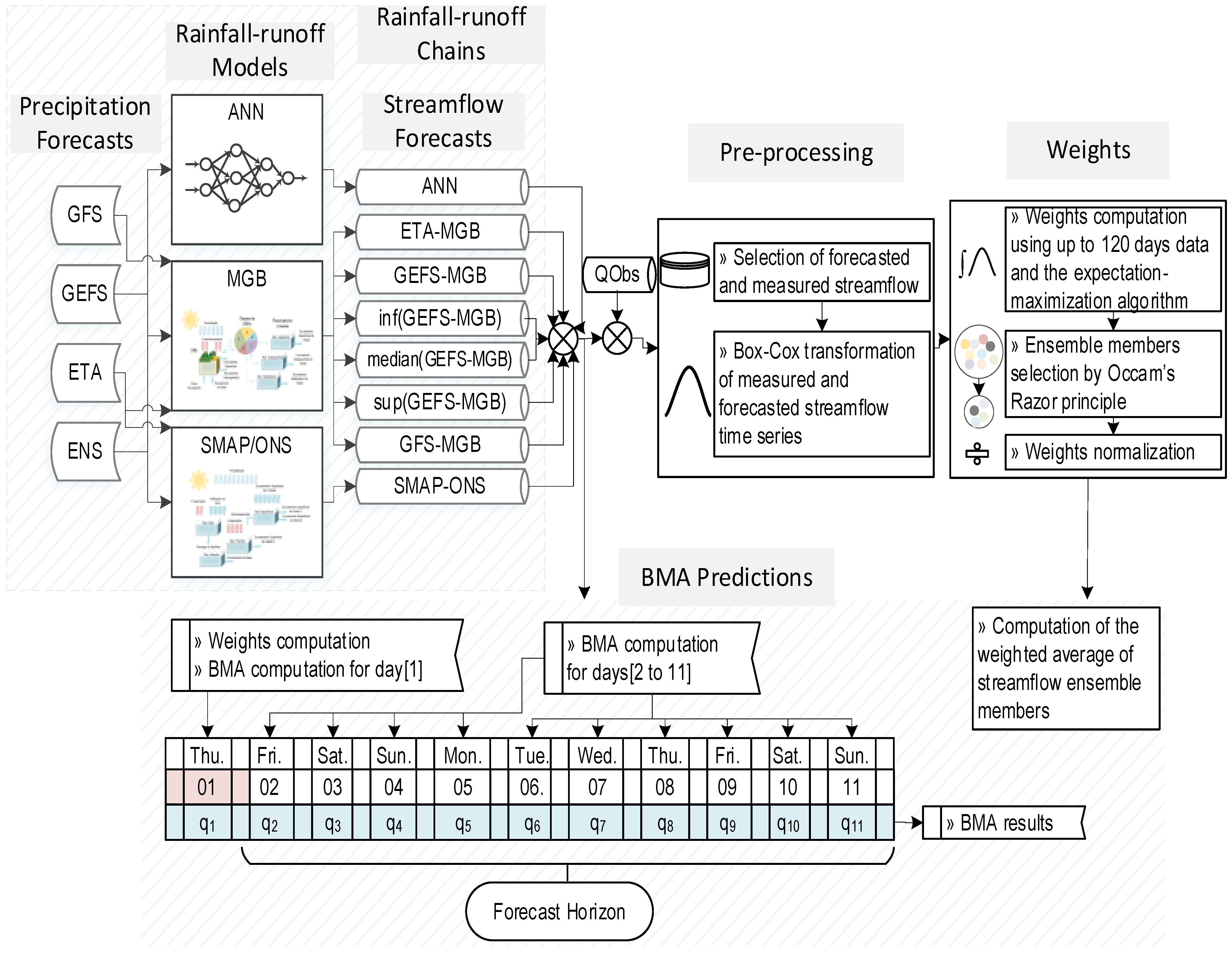
Figure 1. Overview of the proposed Bayesian streamflow ensemble framework.
Water 16 00586 g001
Figure 2. The flowchart of procedures to compute BMA via backtesting simulations is illustrated in (a), and the process to segregate the forecasts made by a rainfall–runoff chain, according to the days of the forecast horizon (day 1, day 2, …, day 11), are exemplified in (b).
Water 16 00586 g002
Figure 3. Reservoirs and hydropower plants of SIN. The long-term natural streamflow average emphasizes the larger plants according to streamflow records from 1931 to 2020.
Water 16 00586 g003
Figure 4. Ensemble weights and natural inflows of Água Vermelha hydropower plant. The first image shows the ensemble members (GFS-MGB, ETA-MGB, GEFS-MGB, inf(GEFS-MGB), median(GEFS-MGB), sup(GEFS-MGB), ANN, and SMAP/ONS), the BMA predictions, and the measured streamflows (QObs) from August 2019 to September 2020. The BMA’s MD is 0.084, which is lower than those computed for the individual ensemble members.
Water 16 00586 g004
Figure 5. MAPE, NSE, and MD were computed using natural inflows to reservoirs and hydropower plants simulated by SMAP/ONS. The backtesting simulation datasets (days 1, 7, and 11) were used to assess the predictive performance of the ensemble members and the BMA for 67 reservoir and hydropower plants. The boxplots show the distributions of MAPE, NSE, and MD in quartiles. The horizontal line inside each box represents the median, while the lines at the lower and upper bounds represent the first quartile (Q1) and third quartile (Q3), respectively. The upper bound of the boxplot is defined by Q3 + 1.5 × (Q3 − Q1) and the lower bound by Q1 − 1.5 × (Q3 − Q1). Colored dots outside the boxes indicate outliers, and a black dot represents the mean. For better visualization of the results, the y-axis scale of each plot underwent a transformation process using the cubic root function  y 3 .
Water 16 00586 g005
Figure 6. Spatial patterns of MD computed with BMA’s forecasts for days 1, 7, and 11.
Water 16 00586 g006
Figure 7. Spatial pattern of  1 C D F D M T c a l c  from Diebold–Mariano test for an 11-day forecast horizon. Each map compares an ensemble member’s predictions with those of the BMA. If  0 1 C D F D M T c a l c < 0.05 , the time series of predictions made by the BMA is significantly more accurate than the competing ensemble member, where  1 C D F D M T c a l c  represents the p-value from hypothesis test (12) at  α = 0.05 ; if  0.05 1 C D F ( D M T c a l c ) 0.95 , none of the time series are significantly more accurate than the others; and, if  0.95 < 1 C D F ( D M T c a l c ) 1 , the time series of predictions made by the multi-model ensemble member is statistically more accurate than the time series of predictions made by BMA, where  C D F D M T c a l c  represents the p-value from hypothesis test (11) at  α = 0.05 .
Water 16 00586 g007
Figure 8. BMA weights for reservoirs and hydropower plants with natural inflows: (a). simulated by SMAP/ONS and (b). not simulated by SMAP/ONS. Black squares represent the average values in each boxplot, and the colored dots represent the outliers.
Water 16 00586 g008
Figure 9. Boxplots of weights computed for (a). GEFS-MGB, (b). ANN, and (c). SMAP/ONS considering the 67 reservoirs and hydropower plants with natural inflows simulated by the SMAP/ONS chain. Black squares represent the average values in each boxplot, and the colored dots represent the outliers.
Water 16 00586 g009
Figure 10. Boxplots of weights computed for (a) ETA-MGB, (b) GEFS-MGB, and (c) ANN considering the 72 reservoirs and hydropower plants, with natural inflows not simulated by the SMAP/ONS chain. Black squares represent the average values in each boxplot, and the colored dots represent the outliers.
Water 16 00586 g010
Table 1. Numerical weather forecast systems.
ModelDetails
GFSThe Global Forecast System (GFS) is a global numerical weather prediction system that has been operational at the National Centers for Environmental Prediction (NCEP) since 1991 [37]. The system couples individual numerical models of atmosphere, ocean, land, and sea ice to portray the weather conditions using atmospheric and land–soil variables [38], thereby establishing itself as one of the state-of-the-art numerical systems that are capable of running at various spectral resolutions [39]. At NCEP, this integrated system of models runs four times daily—at 00, 06, 12, and 18 UTC—producing deterministic scenarios with a forecast horizon of up to 16 days [40]. In the present study, we use the total precipitation data from the GFS’s 18 UTC runs [41], provided at a horizontal spatial resolution of 0.25° latitude by 0.25° longitude.
GEFSThe Global Ensemble Forecast System (GEFS) is a global numerical weather forecasting system developed by NCEP that generates predictions up to 16 days in advance. The 11.0 version of the system was actively used for forecasting from December 2016 until September 2020. During its operational period, GEFS generated 21 different precipitation scenarios (i.e., ensemble prediction). The first one is the base scenario or the control member, and the remaining ones underline uncertainties from the input data, such as limited coverage, instruments, or observing system biases [42], by using a breeding method to introduce perturbations in the initial conditions [43]. In the present study, we use the total precipitation data from the GEFS’s 18 UTC runs [44] in a horizontal spatial resolution of 1° latitude by 1° longitude.
ETAThe η (ETA, from Greek alphabet) is a regional numerical weather forecasting model developed by the University of Belgrade in collaboration with the Institute of Hydrometeorology of Yugoslavia [45]. The ETA model became operational at CPTEC (Center for Weather Forecasting and Climate Studies) in the 1990s and has been used since then to forecast the South American weather. The model’s name refers to a vertical coordinate η that represents the vertical structure of the atmosphere, taking the sea level as a reference [46]. Initially, the ETA model was developed only to make regional weather predictions, but it was later successfully applied in climate prediction and projection studies [47]. The operational version of the ETA model used to forecast the weather conditions of South America has a horizontal spatial resolution of 0.4° of latitude × 0.4° of longitude, as well as a forecast time horizon of 11 days ahead. Unfortunately, the daily forecasts made by the ETA model were downloaded using a link that is no longer available. The precipitation data from the ETA model are now available through the SINtegre portal [48].
ENSThe ensemble forecast (ENS) consists of an ensemble of possible future weather states, generated by the ECMWF Integrated Forecast System [49]. This ensemble includes one control/unperturbed member and fifty disturbance members, all of which are produced twice daily, at 00 and 18 UTC, by the IFS at the European Climate Center. The ECMWF IFS is a numerical system composed of several coupled components that model the atmosphere, ocean, wind-generated ocean waves, sea ice, land surface, and lakes to predict the evolution of the climate system [50]. In this study, we use the ENS total precipitation dataset, which provides forecasts extending 15 days ahead and has a horizontal resolution of 0.20° latitude by 0.20° longitude. Although the original product was an ensemble of predictions, we did not have access to the individual members, but to the average, through the SINtegre portal [51].
Table 2. Evaluation metrics and hypothesis test.
Metric/TestDetails
MAPEThe mean absolute percentage error (MAPE) (7), as outlined in [92], is a metric to measure the predictive accuracy of a time series. According to criteria established in [92], a MAPE between 0 (0%) and 0.1 (10%) indicates high accuracy, values between 0.1 (10%) and 0.2 (20%) indicate good accuracy, values between 0.2 (20%) and 0.5 (50%) indicate reasonable accuracy, and values above 0.5 (50%) indicate poor accuracy.
M A P E = 1 T t = 1 T x m , t y t y t
where  x m , t  is the forecast made by model  m  and  y t  is the measured value.
NSEThe Nash–Sutcliffe efficiency coefficient (NSE) [93], (8), is a metric to evaluate the efficiency of rainfall–runoff models. It measures the ratio of the residual variance (i.e., the residual sum of squares) to the variance of the measured value dataset (i.e., the total sum of squares) subtracted from 1. NSE ranges from 1 to  . The interpretation of NSE is also based on predefined intervals [94,95]. Values above 0.75 indicate that the model has very good efficiency, values between 0.65 and 0.75 indicate good efficiency, values between 0.5 and 0.65 indicate satisfactory efficiency, and values less than 0.5 indicate unsatisfactory efficiency. Additionally, NSE values below zero also suggest that the mean of measured values is a better forecast than the predictions performed by the model under evaluation.
N S E = 1 t = 1 T x m , t y t 2 t = 1 T y t y ¯ 2
where  x m , t  is the prediction made by model  m y t  is the measured value, and  y ¯  is the average of a set of measured values.
MDMulti-criteria distance (MD) [96], (9), has been the metric officially used by ONS to assess streamflow forecasts since 2010. MD is defined as the Euclidean distance between two points,  p 1 = ( x p 1 , y p 1 )  and  p 2 = ( x p 2 , y p 2 ) , calculated as  d = x p 1 x p 2 2 + y p 1 y p 2 2 . Here, the first point  p 1  represents the ideal values of MAPE and NSE (i.e.,  x p 1 = 0  and  y p 1 = 1 , respectively), while the second point  p 1  represents the actual values of the model being assessed ( x p 2 = M A P E  and  y p 2 = N S E ). MD ranges from 0 to  . The higher its value is, the worse the performance of the assessed model is. Therefore, the optimal MD value is zero.
M D = M A P E 2 + 1 N S E 2
Diebold–Mariano testThe Diebold–Mariano hypothesis test [97] is widely used to compare the predictive accuracy of a pair of time series, A and B, using the difference between the measured data and the predictions ( e A , t  and  e B , t ). A loss function  l o s s .  of absolute or quadratic error over time is computed for each time series,  l o s s ( e A , t )  and  l o s s ( e B , t ) , and the gap between them is known as differential loss function  d t = l o s s e A , t l o s s e B , t . In the original version of the Diebold–Mariano test (10), if the expectation of  d t  is equal to zero,  E d t = 0  (i.e., null hypothesis  H 0 ), it is said that A has the same level of accuracy as B; otherwise, their accuracies differ,  E d t 0  (i.e., alternative hypothesis  H a ). On the other hand, in the alternative versions of the Diebold–Mariano test (11) and (12),  H 0  and  H a  are changed in order to determine whether series A is more accurate than series B, or if series B is more accurate than series A, respectively. The results are evaluated through the analysis of the p-value, calculated using the statistic  D M T _ c a l c  (13). Values of p-value lower than the significance level  ( α )  indicate that there is sufficient evidence to reject  H 0  and accept  H a , while values of p-value greater than  α  indicate that there is insuficiente evidence for the rejection of  H 0  and acceptance of  H a .
Original hypothesis:
H 0 : E d t = 0 H a : E d t 0 p - value = 2 × 1 C D F D M T c a l c
Modified Hypothesis I:
H 0 : E d t 0 H a : E d t < 0 p - value = C D F D M T c a l c
Modified Hypothesis II:
H 0 : E d t ¬ 0 H a : E d t > 0 p - value = 1 C D F D M T c a l c
Diebold–Mariano statistic:
D M T c a l c = d ¯ γ 0 + 2 k = 1 h 1 γ k n
where CDF is the cumulative distribution function of the  D M T  statistic;  h  is the forecast horizon;  γ k  is the autocovariance of lag  k  related to function  d n  is the total number of data points of each time series; and  d ¯  is the mean value of the differential loss function.
Disclaimer/Publisher’s Note: The statements, opinions and data contained in all publications are solely those of the individual author(s) and contributor(s) and not of MDPI and/or the editor(s). MDPI and/or the editor(s) disclaim responsibility for any injury to people or property resulting from any ideas, methods, instructions or products referred to in the content.