The Reason for the Rise in Critical Shear Stress on Sloping Beds

Abstract

In sediment mechanics, the conditions for the onset of sediment movement are of particular importance. However, despite decades of research, questions remain unanswered. Thus, physical logic suggests that sediments move more easily on beds inclined in the direction of flow than on horizontal beds and that transport rates are correspondingly increased. However, numerous studies have shown that sediments require increased rather than decreased shear stress to move on sloping beds and that transport rates are lower instead of increased. Since an early publication on this issue by Ashida and Michiue in 1973, many possible effects have been suggested for this apparent contradiction. The literature almost consistently concludes that high relative roughness (d/h), i.e., low water cover (h/d), is mainly responsible for this contradictory effect. This is true for current-induced sediment transport and for the initiation of debris flow. In this paper, an analytical solution for the effect of small water coverage on the transport process is developed. Effects of low coverage also occur on beaches during wave runup and runoff and thus control the formation of steep or less steep beaches. The present paper shows that the effect of turbulence damping occurring under low water coverage plays a decisive role here.

1. Introduction

The movement of sediments on river beds is determined by the balance of driving and resisting forces. Driving forces are caused by the friction along the overflowed grain surface, as well as the flow pressure on the considered grain. These quantities depend on the flow velocity and the turbulence condition of the flow. Resisting forces result from the particle weight, its shape and the bedding. The more exposed the latter is, the stronger the flow attack. The critical shear stress (${\tau }_c$) required for the initiation of sediment motion is therefore an essential quantity in sediment mechanics. Fundamental research on this goes back to Shields (1936) [1]. However, the traditional Shields curve only applies to the condition of low bed gradients and large water covers.

In sloping waters, part of the force of gravity is directed parallel to the river bed and, thus, causes a downslope force on the sediments. The steeper the slope, the easier it should be for the sediments to move.

In contrast, however, a large number of measurement results for larger slopes did not show the expected decrease in the critical shear stress required for the beginning of sediment movement. On the contrary, higher shear stresses have been reported for the start of motion than on a horizontal bed (Ashida & Bayazit 1973 [2], Shvidchenko & Pender 2000 [3], Gregoretti 2000 [4], Armanini & Gregoretti 2005 [5], Lamb, Dietrich & Venditti 2008 [6]), Recking 2009 [7], Prancevic, Lamb & Fuller 2014 [8], Prancevic & Lamb 2015 [9,10]) and other researchers cited therein).

For this unexpected result in downslope flow condition, various possible explanations have been proposed and investigated in the literature, such as increased bedding stability on the resisting side or reduced flow loading on the driving side. The former suggestion is excluded according to studies by Prancevic and Lamb 2015 [10]. The probable cause of this unexpected effect of sloping beds is thought to be the shallow water depth (h) relative to the grain size (d) of the bed, as postulated as early as 1973 by Ashida and Bayazit [2] and later by others. Such conditions of low relative water depth (h/d) occur mainly at large gradients, since this is associated with increased flow velocity (v) and, because of the continuity condition, with reduced water depth (h). Thus, there is often a correlation between low h/d and slope. However, no analytical solutions have been presented for the dependence of sediment movement on slope at small $h/d$.

Several of the papers mentioned above concluded that the velocity profiles at low water cover (h/d), which are also understood as high relative roughness (-height) ($d/h$), systematically deviate from the logarithmic profile in deep water. One consequence is that the flow velocities at grain height decrease, as so do the effective shear stresses. Based on the contribution of Zanke 2001 [11], 2003 [12] using a turbulence-based approach to the Shields curve, it is evident that the Shields values are noticeably affected by the water cover as soon as $h⪅100d$. Then a damping of the turbulence occurs, which, in turn, causes a reduction in the effective shear stresses. For debris of, e.g., $d=10$ cm, $h>10$ m would be necessary for this effect to be ineffective. However, because naturally occurring runoff at steep gradients usually causes much smaller relative water depths ($h/d$), runoff at large gradients is usually associated with turbulence damping. The effect of turbulence damping can cancel out or even overcome the effect of the slope.

In this paper, the combined effect of downslope components of weight force and turbulence damping at small cover is discussed, and a solution is provided to the apparent contradiction of often weaker sediment movement at steeper gradients as described above. The focus is on the onset of movement at the bed surface, which starts sporadically with single grains and changes into a general transport at the bed surface with increasing shear stress. This is typical for the beginning of transport in flowing waters. The onset of an abrupt movement of thicker soil layers, such as a debris flow, is physically related but not identical and is not discussed here.

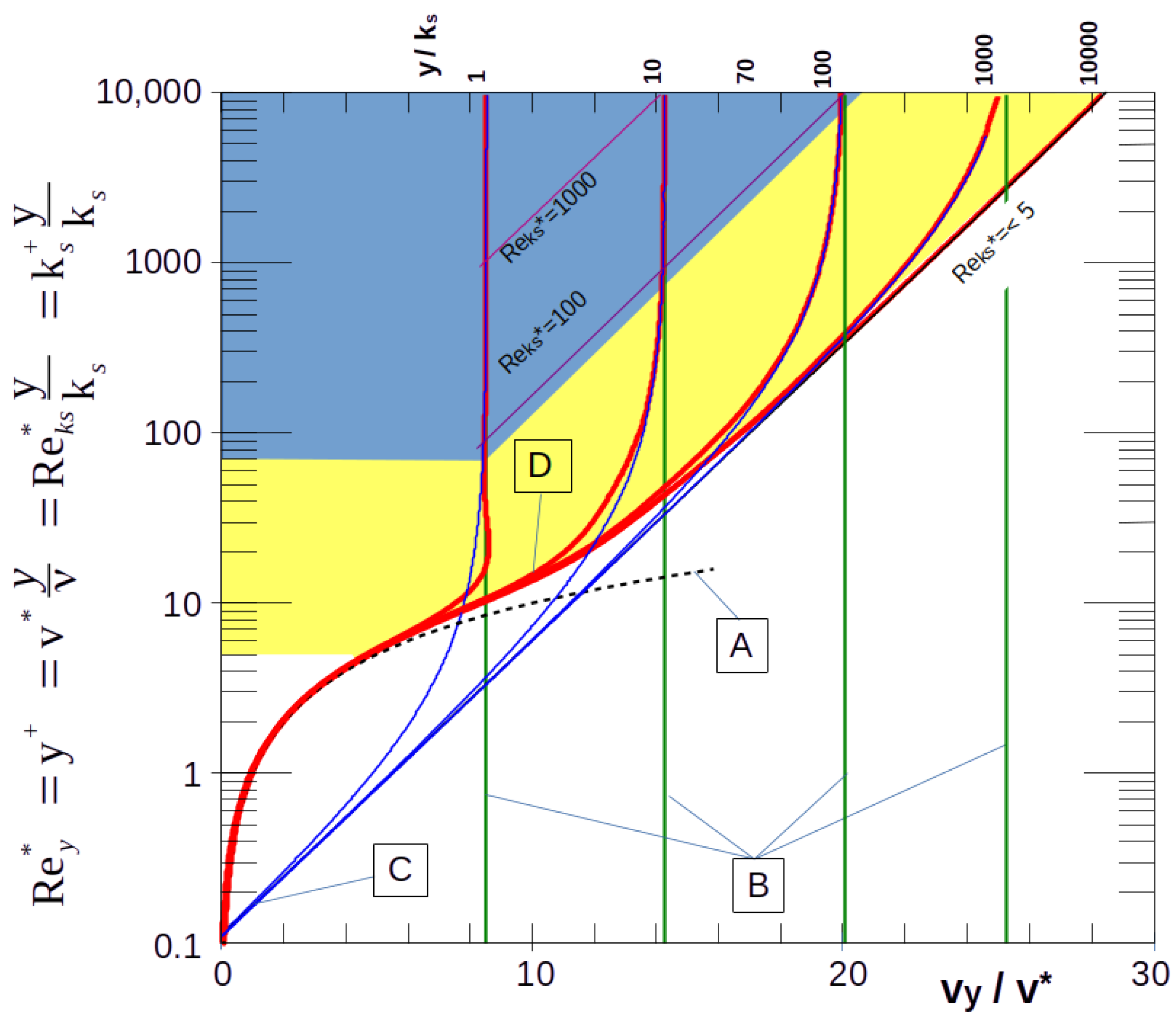
2. Turbulence Damping with Low Water Coverage

If the relative coverage falls below $h/d\approx 100$, noticeable turbulence damping occurs, as previously mentioned. According to Nezu and Rodi (1986) [13], on the basis of different measurements (Laufer 1954 [14], Grass 1971 [15], Eckelmann 1974 [16], Stefffler, Rajaratnam, Peterson 1985 [17], Nezu & Rodi 1986 [13])for different wall distances, this can be described by

$$\frac{v_{rms}^{\prime }\left(y\right)}{v^{★}}=0.3y^{+}{e}^{-0.1y^{+}}+2.26e^{-0.88\frac{y}{h}}(1-e^{-0.1y^{+}})$$

(1)

where $v_{rms}^{\prime }\left(y\right)$ is the fluctuation quantity of the flow velocity at the wall distance, Furthermore $v^{★}$ is the shear stress velocity, $\sqrt{\tau /\rho }$, $\tau$ is the shear stress at the bed, $y^{+}=y\frac{v^{★}}{\nu }$ is the dimensionless wall distance, $\nu$ is the kinematic viscosity and $(1-e^{-0.1y^{+}})=\Gamma$ is the v. Driest damping coefficient modified according to Nezu & Rodi. Nezu and Nakagawa [18] reproduced measurement results from Grass (1971) [15] and Nezu (1977) (in [15]) for $\frac{v_{rms,y}^{\prime }}{v^{★}}=f\left(y^{+}\right)$ for various roughness conditions ($k_s^{+}$). From these curves, the course of the function $v_{rms,b}^{\prime }/v^{★}=f\left(k_s^{+}\right)$ can be derived for $y=k_s$, as well as for $y^{+}=k_s^{+}$, and described by a modification of the factors in Equation (1) (Zanke 2001 [11], 2003 [12]):

$$\frac{v_{rms,b}^{\prime }}{v^{★}}=0.31k_s^{+}{e}^{-0.1k_s^{+}}+1.8e^{-0.88\frac{k_s}{h}}(1-e^{-0.1k_s^{+}}).$$

(2)

where $k_S$ is the equivalent sand roughness height, and $k_S^{+}=k_S\frac{v^{★}}{\nu }$. The ratio value ($k_S/d$) is assumed to be $k_S/d\approx 1$, so $k_S\approx d$. The subscript ’b’ denotes the position on the bed at $y=k_S$. Under hydraulically rough conditions, $e^{-0.1k_s^{+}}\to 1$, so Equation (2) simplifies to

$$\frac{v_{rms,b}^{\prime }}{v^{★}}=1.8e^{-0.88\frac{k_s}{h}}hydraulical rough.$$

(3)

The functional relationship is shown in Figure 1. Given hydraulically rough conditions with $k_s^{+}⪆70$, $v_{rms,b}^{\prime }/v^{★}$ is only a function of $h/d$ or of $h/k_s$. Below $k_s^{+}\approx 70$, the conditions change towards hydraulically smooth, and $v_{rms,b}^{\prime }/v^{★}$ additionally depends on $k_s^{+}$. Between $k_s^{+}=$ 10 and 20, a maximum occurs, and in the region of $k_s^{+}⪅5$, the near-bed turbulence decreases rapidly as the wall is approached.

Thus, at a relative cover of $h/k_s⪆100$, the water cover has virtually no effect on the value of $v_{rms,b}^{\prime }/v^{★}$. However, under lower cover, the turbulence is increasingly damped. That is, ${\tau }^{\prime }$ is reduced, and the peak values of $\tau =\overline{\tau }+{\tau }^{\prime }$ approach the mean shear stress ($\overline{\tau }$). Figure 2 makes clear that the effective shear stress for the sediments is significantly codetermined by the occurring peak values.

Since it is common to understand $\tau$ as the time average $\overline{\tau }$, the effective shear stress becomes smaller with damped turbulence, despite an unchanged $\tau =\rho ghI$. Therefore, to achieve the same shear effect as in the case of $h/k_s⪆100$, $\tau =\overline{\tau }$ must increase under low coverage, which is equivalent to high relative roughness. Otherwise, the effective shear stress on the bed is reduced to

$${\tau }_{h/k_s}=D_{\tau }{\tau }_{h/k_s>100}.$$

(4)

where ${\tau }_{h/k_S}$ is the shear stress on the bed reduced under the influence of low coverage. The damping coefficient ($D_{\tau }$) describes the reduction factor of the shear stress on the bed. As also $\tau \sim \rho v{’}_{rms,b}^2$, the effective shear velocity at the bed is described by $v_{h/ks}^{★}\sim v^{★}{\left(\frac{v_{rms,b}^{\prime }}{v^{★}}\right)}_{h/k_s}$; thus,

$$D_{\tau }=\frac{{\tau }_{h/k_s}}{{\tau }_{h/k_s>100}}=\frac{{\tau }_{h/k_s}^{★}}{{\tau }_{h/k_s>100}^{★}}={\left(\frac{v^{★}{\left(\frac{v_{rms,b}^{\prime }}{v^{★}}\right)}_{h/k_s}}{v^{★}{\left(\frac{v_{rms,b}^{\prime }}{v^{★}}\right)}_{h/k_s>100}}\right)}^2={\left(\frac{{\left(\frac{v_{rms,b}^{\prime }}{v^{★}}\right)}_{h/k_s}}{{\left(\frac{v_{rms,b}^{\prime }}{v^{★}}\right)}_{h/k_s>100}}\right)}^2$$

(5)

and, in combination with Equation (2), as

$$D_{\tau }={\left(\frac{0.31k_s^{+}{e}^{-0.1k_s^{+}}+1.8e^{-0.88\frac{k_s}{h}}(1-e^{-0.1k_s^{+}})}{0.31k_s^{+}{e}^{-0.1k_s^{+}}+1.81(1-e^{-0.1k_s^{+}})}\right)}^2.$$

(6)

Figure 1 shows that $v’/v^{★}$ is independent of the water coverage if $h/k_s⪆100$.

In engineering practice, relevant cases of low relative water coverage exist, e.g., in mountain streams and rivers, in artificially made steep flow sections, such as rough ramps and, likewise, in the area of wave runup and backwash on coarse-grained beaches. Under such typically hydraulically rough conditions, Equation (6) reduces to

$$D_{\tau }=e^{-1.76\frac{k_s}{h}}hydraulicalrough.$$

(7)

Depending on the ratio of $ks/d$ or $k_s/d_{90}$, the damping effect differs slightly, as Figure 3 shows. (The relation of $k_s/d_{90}$ is introduced here with respect to the data presented in Figure 4).

The logarithmic velocity profile for turbulent flows is based on the assumption of $h\gg k_s$ or $h\gg \delta$. Therefore, it does not cover the range of small relative water depths ($h/k_s$, $h/d$ and $h/\delta$) where turbulence is damped and, hence, velocity profiles are modified.

For profiles with low coverage results (see also Bezzola 2002) [20])

$$\frac{v}{v^{★}}=\sqrt{D_{\tau }}{\left(\frac{v}{v^{★}}\right)}_{h/k_s>100},$$

(8)

i.e., in the hydraulically rough case

$$\frac{v_y}{v^{★}}=\sqrt{D_{\tau }}\left(\frac{1}{\kappa }ln\frac{y}{k_S}+8.5\right)$$

and

$$\frac{v_m}{v^{★}}=\sqrt{D_{\tau }}\left(\frac{1}{\kappa }ln\frac{h}{k_S}+6\right).$$

Various experiments have been reported by different authors on the effect of low coverage on the beginning of sediment movement. In addition to laboratory experiments conducted by Bayazit (1976) [21], (1983) [22] with gravel, idealized spheres or hemispheres as roughness elements, Rickenmann (1996) [23] were used to evaluate measurements from steep streams Ruf 1990 [24], Jarrett 1984 [25], Bathurst 1985 [26], Thompson & Campbell 1979 [27], Thorne & Zevenbergen 1985 [28], Griffith 1981 [29] Comparatively low water covers are typical for such mountain streams. The coverage effect is illustrated in Figure 4 by a variety of data for the parameter $v_m/v^{★}$ as a function of the roughness parameter ($k_s=d_{90}$). Also shown are the solutions of Equation (8) with $D_{\tau }$ according to Equation (7) for the cases of ${(v_m/v^{★})}_{h/d90=100}$ = 16, 11.5 and 7.5.

Figure 4. Measured data from torrents (Rickenmann [23]) and solutions of Equation (8).

Figure 4. Measured data from torrents (Rickenmann [23]) and solutions of Equation (8).

Concerning the shape of the curves, the $k_s/d_{90}$ values given for the respective curves provide the best agreement. These results can also be converted to the dependence on, e.g., $h/d_{50}$. A first approximation of this can be obtained from

Table 1. First estimates of $d_{90}/d_{50}$.

	Lowland Rivers	Mountain Streams
$d_{90}/d_{50}$	$\approx 1.8$	$\approx 3$

.

Figure 5 shows the solution to $D_{\tau }$ for the hydraulically rough case with the bold blue curve (Equation (7)). This curve corresponds to the middle curve in Figure 4. Thus, with $\frac{h}{k_S}=\frac{h}{0.7d_{90}}$ corresponding to the value of $h/d_{90}=x$ in Figure 4, the abscissa value is $h/k_S=1.43x$; for example, in Figure 4, $h/d_{90}=10$ corresponds to the abscissa value of $h/k_S=7$ in Figure 5. The ordinate value in Figure 4 at $h/d_{90}=10$ is about 10.2; therefore, $D_{\tau }={(10.2/11.5)}^2=0.79$ as also at $h/k_S=7$ in Figure 5.

In the case of non-hydraulically rough conditions, a reduced damping effect occurs. Equation (6) also covers this case, as shown in Figure 5 with the curves for different values of $R{e}_{ks}^{★}$.

An adequate empirical solution for the damping factor for exclusively hydraulically rough flows was also developed by Bezzola (2002) [20] based on the concept of a “roughness sublayer” of thickness $y_R$ defined in 1981 by Raupach [30] in which the separations at the roughness elements determine the turbulence characteristics. In this roughness sublayer, the shear stress no longer increases linearly toward the bottom but is approximately constant over the layer thickness ($y_R$) (Figure 6). As a result, the shear stress at the bed is reduced with a damping factor ($D_{\tau }$), which is

$$\begin{array}{c}\hfill D_{\tau }=\frac{h-y_R}{h}\end{array}$$

(9)

where $y_R=\alpha k$ and k is the geometric roughness height of the roughness elements at the bed. However, when $h<y_R$, Equation (9) yields negative values. Assuming a linear curve for $h/y_R\le 2$, Bezzola recommends

$$\frac{h}{y_R}>2D_{\tau }=1-\frac{y_R}{h}\mathrm{Bezzola}$$

(10)

$$\frac{h}{y_R}\le 2D_{\tau }=0.25\frac{h}{y_R}\mathrm{Bezzola}$$

(11)

Bezzola’s solution of is shown in Figure 5, as represented by the dashed red curve. A difficult problem is to determine the thickness of the roughness sublayer ($y_R$), which depends on the size (d) of the grains and stones, as well as their shape and arrangement. The data reported by Bezzola are in the range of $0.5⪅y_R/d⪅2$ with $y_R\approx 1.5d$ for natural sediment surfaces.

Independently, Lamb, Brun and Fuller (2017) [31] also concluded that flow resistance increases significantly with increasing relative roughness, which is consistent with Equation (8).

3. Beginning of Sediment Movement

3.1. Measurement Data on the Beginning of Movement at a Large Gradient and Low Water Cover

As previously mentioned, the work of many researchers led to the unexpected result that large slopes do not necessarily lead to a reduction in the shear stress critical for the beginning of movement but, on the contrary, an increase.

This finding applies to the first particles starting to move on the surface of a sediment bed, as well as to the abrupt initiation of movement of thicker soil layers in the form of debris flows.

Published measurements for which sufficient accompanying data are provided, such as density, friction angle and critical shear stress, in the standard case of very low slope are comparatively rare.

Table 2. Measured influence of slope and low water coverage on the initiation of movement and calculated values (${\tau }_{c,h/d,\alpha }^{★}/{\tau }_{c,\infty ,0}^{★}=\eta /D_{{\tau }_c}$). Green background: direct data information or extracted from the data. yellow: estimated; red: calculated on the basis of the data and estimated values.

	A	B	C	D	E	F	G	H	I	J	K	L	M	N	O	P	Q
Nr.	Author	$\mathit{\alpha }$	$\mathit{\phi }$	$\mathit{\eta }$	h	d	${\mathit{\rho }}^{\prime }$	h/d	$\frac{\mathbf{1}}{{\mathit{D}}_{{\mathit{\tau }}_{\mathit{c}}}}$	$\frac{\mathit{\eta }}{{\mathit{D}}_{{\mathit{\tau }}_{\mathit{c}}}}$	${\mathit{\tau }}_{\mathit{c},\mathit{h}/\mathit{d},\mathit{\alpha }}^{★}$	${\mathit{\tau }}_{\mathit{c},\infty ,\mathbf{0}}^{★}$	${\mathit{\phi }}_{\mathit{d}}$	$\mathit{\alpha }/{\mathit{\phi }}_{\mathit{d}}$	$\frac{\mathbf{1}}{{\mathit{D}}_{{\mathit{\tau }}_{\mathit{c}}}}$	$\frac{\mathit{\eta }}{{\mathit{D}}_{{\mathit{\tau }}_{\mathit{c}}}}$	P/J
	-	o	o	-	m	m	-	-	-	-	-	-	o	-	-	-	-
1	Ashida	1.15	45.0	0.959	0.091	0.0225	1.65	4.07	1.182	1.134	0.0431	0.038	26.5	0.043	1.2416	1.191	1.051
2	&	2.86	45.0	0.899	0.036	0.0225	1.65	1.58	1.542	1.385	0.0527	0.038	26.5	0.108	1.7467	1.570	1.133
3	Bayazit	4.30	45.0	0.847	0.025	0.0225	1.65	1.11	1.891	1.601	0.0607	0.038	26.5	0.162	2.2078	1.869	1.168
4	[2]	5.70	45.0	0.796	0.022	0.0225	1.65	0.96	2.451	1.950	0.0743	0.038	26.5	0.215	2.5116	1.998	1.025
5	“	8.50	45.0	0.692	0.015	0.0225	1.65	0.68	3.395	2.350	0.0894	0.038	26.5	0.321	3.6478	2.525	1.074
6	“	11.30	45.0	0.587	0.013	0.0225	1.65	0.58	5.279	3.099	0.1178	0.038	26.5	0.427	4.5863	2.693	0.869
7	“	0.57	45.0	0.980	0.097	0.0125	1.65	8.15	1.079	1.057	0.0402	0.038	26.5	0.022	1.1144	1.092	1.033
8	“	1.43	45.0	0.950	0.036	0.0125	1.65	3.04	1.183	1.124	0.0427	0.038	26.5	0.054	1.3355	1.268	1.129
9	“	2.86	45.0	0.899	0.020	0.0125	1.65	1.71	1.565	1.406	0.0535	0.038	26.5	0.108	1.6738	1.504	1.070
10	“	4.30	45.0	0.847	0.014	0.0125	1.65	1.21	1.891	1.601	0.0608	0.038	26.5	0.162	2.0715	1.754	1.095
11	“	5.70	45.0	0.796	0.012	0.0125	1.65	1.00	2.283	1.816	0.0691	0.038	26.5	0.215	2.4109	1.918	1.056
12	“	7.10	45.0	0.744	0.011	0.0125	1.65	0.96	2.993	2.227	0.0846	0.038	26.5	0.268	2.5049	1.864	0.837
13	“	0.57	52.0	0.983	0.054	0.0064	1.65	8.00	1.033	1.016	0.0386	0.038	30.6	0.019	1.1089	1.090	1.073
14	“	1.43	52.0	0.957	0.024	0.0064	1.65	3.75	1.265	1.211	0.0461	0.038	30.6	0.047	1.2645	1.211	1.000
15	“	2.86	52.0	0.914	0.013	0.0064	1.65	2.03	1.571	1.437	0.0536	0.038	30.6	0.094	1.5422	1.410	0.981
16	Prancevic	1.8	45.6	0.946	0.021	0.015	1.65	1.420	1.198	1.133	0.034	0.030	30.4	0.059	1.8584	1.758	1.551
17	&	3.2	45.6	0.903	0.016	0.015	1.65	1.073	1.734	1.567	0.047	0.030	30.4	0.105	2.2702	2.051	1.309
18	Lamb	5.6	45.6	0.829	0.010	0.015	1.65	0.693	2.453	2.033	0.061	0.030	30.4	0.184	3.5581	2.949	1.450
19	&	5.9	45.6	0.819	0.010	0.015	1.65	0.680	2.571	2.107	0.063	0.030	30.4	0.194	3.6478	2.989	1.419
20	Fuller	6.8	45.6	0.791	0.011	0.015	1.65	0.713	3.160	2.500	0.075	0.030	30.4	0.224	3.4337	2.717	1.087
21	[8]	8.0	45.6	0.753	0.009	0.015	1.65	0.613	3.541	2.667	0.080	0.030	30.4	0.263	4.1987	3.162	1.186
22	[32]	9.8	45.6	0.695	0.009	0.015	1.65	0.620	4.459	3.100	0.093	0.030	30.4	0.322	4.1345	2.875	0.927
23	“	11.5	45.6	0.640	0.009	0.015	1.65	0.587	5.832	3.733	0.113	0.030	30.4	0.378	4.4817	2.869	0.768
24	“	12.4	45.6	0.611	0.007	0.015	1.65	0.487	5.950	3.633	0.109	0.030	30.4	0.408	6.0996	3.725	1.025
25	“	13.5	45.6	0.574	0.007	0.015	1.65	0.467	6.731	3.867	0.116	0.030	30.4	0.444	6.5911	3.786	0.979
26	“	14.2	45.6	0.551	0.007	0.015	1.65	0.480	7.557	4.167	0.125	0.030	30.4	0.467	6.2547	3.448	0.828
27	“	15.6	45.6	0.505	0.007	0.015	1.65	0.487	9.179	4.633	0.139	0.030	30.4	0.513	6.0996	3.079	0.665
28	“	16.9	45.6	0.461	0.006	0.015	1.65	0.433	10.260	4.733	0.141	0.030	30.4	0.556	7.6199	3.515	0.743
29	“	19.6	45.6	0.370	0.007	0.015	1.65	0.493	16.023	5.933	0.178	0.030	30.4	0.645	5.9523	2.204	0.371
30	Prancevic	0.7	-	-	0.0164	0.023	0.15	0.714	-	-	0.058	-	-	-	3.4354	-	-
31	&	0.9	-	-	0.0162	0.023	0.15	0.704	-	-	0.074	-	-	-	3.4882	-	-
32	Lamb	1.4	-	-	0.0155	0.023	0.15	0.676	-	-	0.110	-	-	-	3.6907	-	-
33	[10]	0.7	-	-	0.0135	0.023	0.15	0.588	-	-	0.048	-	-	-	4.4784	-	-
34		0.9	-	-	0.0159	0.023	0.15	0.690	-	-	0.072	-	-	-	3.5714	-	-
35		1.4	-	-	0.0155	0.023	0.15	0.676	-	-	0.110	-	-	-	3.6907	-	-

lists data that fully or largely satisfy the above requirements. The data include bottom slopes of up to about 20 degrees.

For the classification of large gradients, the gradient conditions on the river Rhine are compared. For the first roughly 100 km, the Alpine Rhine has an average bed slope angle of about 0.5 degrees. The value drops to 0.03 degrees in the area of the Upper Rhine and to about 0.007 degrees in the Lower Rhine. In this sense, large slopes are angles of inclinations of more than 0.5 degrees.

Table 2 shows the measured results with a green background. The dynamic angles of the internal friction (${\phi }_d$), which are highlighted in yellow, had to be estimated here. Calculated values for the critical shear stress are highlighted in red. Columns “N, O and P” show the calculated increase factors of the critical shear stress, and column “Q” indicates the quality calculated by means of the quotient “calculated/measured”.

The critical shear stresses in the comparative case of a horizontal bed with large water coverage were taken from the data reported by Ashida and Bayazit. With respect to the data reported by Prancevic et al. (2014) [8], these values had to be recalculated. It should also be mentioned that the values measured by of Prancevic et al. [8] required modification of the given water depths (h) by reducing them by $1/3d$. This yielded reasonable calculation results (see below). Against the background of the very wavy “water level” in photographs presented in the papers by Prancevic et al. [8], at water depths in the order of the grain sizes, this is quite reasonable because accurate water depth measurements are impossible under the reported circumstances.

3.2. Shields Curve

A general solution to the onset of sediment movement was published by Shields in 1936 [1] in the form of a curve (${\tau }_c^{★}=f\left(R{e}^{★}\right)$) obtained from measured data with a Shields number of ${\tau }^{★}=\frac{\tau }{({\rho }_s-\rho )gd}$ and $R{e}^{★}=v^{★}d/\nu$. The Shields curve represents a low degree of movement of cohesion-free sediments for horizontal beds or very small gradients. It further applies to water covers ($h/d$) that have no effect on the critical shear stresses.

3.3. Analytical Solution of the Shields Curve

3.3.1. Turbulence-Free Flow

According to Zanke (2001) [11]/2003 [12], the beginning of sediment motion can be described by an analytical solution, according to which (hypothetically) turbulence-free flow applies.

$${\tau }_c^{★}=(1-p)tan{\phi }_{d}K\eta$$

(12)

where p is the pore fraction, ${\phi }_d$ is the dynamic angle of the internal friction of the sediment and K is the influence of any cohesion present in the sediment. In cohesionless sediment, $K=1$, and at very low slope, $\eta \approx 1$. The influence of a sloping bed is described by

$$\eta =\frac{sin(\phi -\alpha )}{sin\left(\phi \right)}=cos\left(\alpha \right)\left(1-\frac{tan\left(\alpha \right)}{tan\left(\phi \right)}\right)$$

(13)

where $\alpha$ is the angle of inclination of the bottom, which is positive in the downhill direction. For practical purposes, with ${\phi }_d⪅{40}^{\circ }$, the following can be substituted approximately:

$$\eta =1-\frac{\alpha }{\phi }$$

(14)

where ${\phi }_0$ is the static angle of the internal friction; when ${\phi }_0$ is exceeded, the sediment surface slides down abruptly in a layer with a thickness of many grains. $\phi ={\phi }_d$ describes the dynamic angle of internal friction, beyond which particles on the sediment surface can be kept in motion. In the case of moving sediment, φ_d is effective.

3.3.2. Turbulent Flow

Turbulent flows can be characterized by a time averaged (v) and velocity fluctuations ($v^{\prime }$), the latter of which also causes shear stress fluctuations (${\tau }^{\prime }$) (or, in dimensionless form, ${\tau }^{\prime ★}$). If the average shear stress is lower and is insufficient to cause sediment movement, the peak values of the fluctuations are decisive in triggering sediment movement. This is illustrated by the left part of Figure 7. In the right figure, it becomes clear that a higher mean shear stress is required to initiate sediment motion for the lower-turbulence case.

According to Zanke 2001 [11] and 2003 [12], the beginning of sediment movement can be expressed by

$${\tau }_{c,h/ks,\alpha }^{★}=\frac{(1-p)tan{\phi }_{d}K\eta }{{\left(1+n\frac{v_{rms,b}^{\prime }}{v^{★}}\frac{v^{★}}{v_b}\right)}^2\left(1+0.4{\left(n\frac{v_{rms,b}^{\prime }}{v^{★}}\right)}^{2}tan{\phi }_d\right)}$$

(15)

The value of $0.4$ in the function results from the reciprocal of the maximum value (≈2.5) in Figure 1, which is also reduced for small coverage. Because Equation (15) is based on the effect of turbulence, it also includes the effect of turbulence damping. Depending on the hydraulic condition (hydraulically rough or not rough), $v_{rms,b}^{\prime }/v^{★}$ is provided by Equation (2) or (3). The value of n (Figure 7) defines a multiple of $v_{rms}^{\prime }$ at which sediment motion occurs to a certain degree. Larger values of n account for stronger (but more rare) ${\tau }^{\prime ★}$. A value of $n=1.8$ reproduces the Shields curve. For cases in which no turbulence exists ($n=0$), the denominator becomes 1, and Equation (15) reduces to Equation (12). Thus, the critical shear stress is not a hard threshold at which the rest state abruptly changes to the full motion state. Rather, the onset of sediment motion spans a range of $0.5⪅{\tau }^{★}/{\tau }_c^{★}⪅1.5\dots 2$, where Shields ${\tau }_c^{★}$ is a reference value for the beginning of the movement, as previously stated.

In the literature, the critical shear stress for a flat bed with large water cover is given in the range of $0.03⪅{\tau }_c^{★}⪅0.06$. This range is, on the one hand, justified by different angles of the internal friction of the considered sediments and, on the other hand, depends on the degree of movement, which is defined as “beginning”. The first movement occurs when grains with little bedding stability can be set in motion. When the shear stress is further increased, particles that are somewhat more stably supported also begin to move, and so on. Once some grains are in motion, they bump other grains and can thereby increase the degree of motion. For the Shields curve with ${\tau }_c^{★}\approx 0.05$ in the range of $R{e}^{★}>70$, according to Zanke 1989 [33], the degree of motion ≈10%. Figure 8 shows exemplary solutions for $n=1.8$ and $n=3$ for different levels of water coverage ($h/d$). Depending on the internal friction angle (${\phi }_d$) determined by grain size, grain shape and grain surface roughness, the curves shift up or down.

The decreasing effect of turbulence damping towards smaller $R{e}_d^{★}$ values becomes understandable against the background of the viscous sublayer of the boundary layer (relative thickness $\delta /d\approx 11.63/R{e}_d^{★}$) reducing the effective grain roughness and making it largely disappear at $R{e}^{★}⪅5$. Reduced effective grain roughness also indicates a smaller roughness sublayer and, therefore, less turbulence damping. Figure 8 reflects this.

The ratio of the flow velocity directly at the bed ($v_b$) to the shear velocity needed to solve Equation (15); $v_b/v^{★}$ in the turbulent flow domain can be determined via the logarithmic velocity profile:

$$\frac{v_y}{v^{★}}=\left(2.5ln\left(\frac{y}{k_s}\right)+B\right)turbulent$$

(16)

and B can be obtained for natural roughness according to

$$B=2.5ln\frac{1}{0.033+\frac{0.11}{k_s^{+}}}naturally rough$$

(17)

A solution proposed by Zanke (1996) [34] covers the whole range of viscous flow, from turbulent–smooth to turbulent–rough:

$$\frac{v_y}{v^{★}}={\left({\left(\frac{v^{★}}{\nu }y\right)}^{-2}+P_{yt}{\left(2.5ln\left(\frac{y}{k_s}\right)+B\right)}^{-2}\right)}^{-1/2}viscous-turbulent.$$

(18)

where, according to [35], $P_{yt}$ is the probability of turbulence at the wall distance (y).

$$P_{yt}=1-exp\left(-0.08\frac{v^{★}y}{\nu }\right).$$

(19)

Therefore,

$$\frac{v_y}{v^{★}}={\left({\left(\frac{v^{★}}{\nu }y\right)}^{-2}+P_{yt}{\left(2.5ln30\frac{y}{k_s+3.32\frac{\nu }{v^{★}}}\right)}^{-2}\right)}^{-1/2}viscous-turbulent.$$

(20)

Figure 9 shows the course under hydraulically rough, hydraulically smooth and viscous conditions and the respective transitions. A similar solution, although valid only for the viscous–hydraulically smooth transition, was proposed by Reichardt (1951) [36] and is almost congruent with the corresponding result of Equation (20). Directly at the bed, at $y=k_S$, according to [11,12], the following applies:

$$\frac{v_b}{v^{★}}=0.8+0.9\frac{v_{y=ks}}{v^{★}}.$$

(21)

3.4. Angle of Internal Friction Determining the Onset of Motion

The governing angle of internal friction ($\phi$) is of importance for the considerations of transport initiation. The static angle (${\phi }_o$) corresponds to the angle of repose of a dry or completely submerged sediment mass. When it is exceeded, the sediment slides down like an avalanche. The sliding stops when the angle of repose falls below the dynamic angle (${\phi }_d$) of internal friction, which is naturally smaller than the static angle. Static and dynamic friction angles correspond to static and sliding friction coefficients. If a shear stress due to overflow is added, sliding can begin at a lower bottom slope. According to measurements performed by Prancevic et al. (2014) [8], a transition region exists between ${\phi }_d<\phi <{\phi }_o$, where fluvial transport at the bed surface transitions to failure of a thicker layer. For the sediment surface grains, ${\phi }_d$ is decisive. Their individual position angle corresponds to the respective value of ${\phi }_d$.

The first particles to start moving at ${\tau }^{★}\approx 0.5{\tau }_c^{★}$ are particularly unstably supported. Accordingly, they have a small friction angle, which can be even smaller than the dynamic friction angle. Finally, as the intensity of motion increases, dynamic friction becomes effective at the moving surface of the top of the bed.

Based on these considerations, the dynamic friction angle ($\tan {\phi }_d$) is used as the determining factor for the onset of transport.

It is stated in the literature that ${\phi }_d$ is between 2^o and 8^o below ${\phi }_o$ (Bagnold 1941, Allen 1970, 1972, cited in Hanes & Inman [39]). However, it can also be as low as ${\phi }_d\approx 0.5{\phi }_o$ (Madsen 1991 [40], Nino & Garcia 1998 [41]).

3.5. Turbulence Damping and Critical Shear Stress

As discussed in Section 2, the critical shear stresses obviously apply

$${\tau }_{c,h/ks,\alpha }^{★}={\tau }_c^{★}\frac{\eta }{D_{\tau }}$$

where $D_{\tau }$ depends on the flow condition according to Equation (6) or Equation (7), and ${\tau }_c^{★}$ is the critical shear stress on a flat bed ($\alpha \approx 0^o)$ in deep water ($h/d\to \infty ,D_{\tau }=1$). However, for three reasons, $D_{{\tau }_c}$ slightly deviates from $D_{\tau }$ in the critical case:

$${\tau }_{c,h/ks,\alpha }^{★}={\tau }_c^{★}\frac{\eta }{D_{{\tau }_c}}$$

(22)

3.5.1. Finite Critical Shear Stress with Complete Damping of Turbulence

For vanishing water cover, $h/d\to 0$, $D_{\tau }\to 0$ (cf. Figure 5), from which it follows that for the critical shear stress, $\frac{{\tau }_{c,h/d}}{{\tau }_c}\to \infty$. According to Equation (12) and Figure 8, however, it is clear that even with full damping of the turbulence, there still remains a finite critical shear stress, namely the viscous shear stress.

Substituting the attenuation factors ($D_{\tau }$) for low coverage listed in Section 2 into Equation (15), the following is obtained

$${\tau }_{c,h/d,\alpha }^{★}=\frac{(1-p)tan{\phi }_{d}K\eta }{{\left(1+n\sqrt{D_{\tau }}\frac{v_{rms,b}^{\prime }}{v^{★}}\frac{v^{★}}{\sqrt{D_{\tau }}{v}_b}\right)}^2\left(1+\frac{0.4}{D_{\tau }}{\left(n\sqrt{D_{\tau }}\frac{v_{rms,b}^{\prime }}{v^{★}}\right)}^{2}tan{\phi }_d\right)}$$

Thus, $D\tau$ truncates out completely. Therefore, Equation (15) already fully describes the effect of low coverage. Therefore, for $D_{{\tau }_c}$, it from Equation (15) that

$$\frac{{\tau }_{c,h/d,\alpha }^{★}}{{\tau }_{c,\infty ,0}^{★}}=\frac{\eta }{D_{\tau ,c}}=\frac{\eta {\left[{\left(1+1.8\frac{v_{rms,b}^{\prime }}{v^{★}}\frac{v^{★}}{v_b}\right)}^2\left(1+0.4{\left(1.8\frac{v_{rms,b}^{\prime }}{v^{★}}\right)}^{2}tan{\phi }_d\right)\right]}_{h/d>100}}{1{\left[{\left(1+1.8\frac{v_{rms,b}^{\prime }}{v^{★}}\frac{v^{★}}{v_b}\right)}^2\left(1+0.4{\left(1.8\frac{v_{rms,b}^{\prime }}{v^{★}}\right)}^{2}tan{\phi }_d\right)\right]}_{h/d}}$$

(23)

3.5.2. Turbulence Damping for Exposed Particles

A comparison with measured critical shear stresses shows that a lower damping is effective for the beginning of motion than that for the general bed described above. In other words, the damping factors ($D_{{\tau }_c}$) at the level of the particles moving over the bed are larger than $D_{\tau }$ at the general bed at $y=0$ (keep in mind: larger damping factor = lower damping). This was also stated by Bezzola (2002) [20].

The reason for this phenomenon is that the particles with little stability are decisive for the flow-induced initiation of motion at the surface of the bed. These protrude above the bottom and are therefore affected by lower turbulence damping compared to the general bottom. Figure 10 illustrates this. At the bed, the loss of shear stress is ${\tau }_0(1-D_{\tau })$, and at the moving grain, it is only $\approx {\tau }_0(1-D_{\tau })/2$. In other words, for the beginning of motion, $D_{{\tau }_c}$ is to be referred to as $ks/d\approx 0.5$ or $y_R/d\approx 0.75$ instead of $ks/d\approx 1$ or $y_R/d\approx 1.5$ when referring to the bed at $y=0$.

Based on the measured $\eta$ and ${\tau }_c^{★}$ values, $D_{{\tau }_c}=\eta /{\tau }_c^{★}$ adjusted for the slope effect can be obtained. Figure 11 shows such results from data reported by Ashida and Bayazit (1973) [2]. The courses of Equations (7) and (23) for $k_S/d=1$ and $k_S/d=0.5$ are also shown. In agreement with Figure 10, the measured values are smaller than the values of $1/D_{\tau }$ and are represented by the solutions of Equations (7) and (23) based on $k_S/d=0.5$.

3.5.3. Degree of Movement at Start of Movement

The relation $\frac{{\tau }_{c,h/d}^{★}}{{\tau }_{c,\infty ,0}^{★}}$ depends on the degree of motion assumed for the beginning of the grain motion, e.g., a small but already distinct motion, as for a Shields curve with $n\approx 1.8$ and ${\tau }_c^{★}\approx 0.052$ or with much lower intensity of motion at $n\approx 3$ and ${\tau }_c^{★}\approx 0.019$. In the former case at, for example, $h/d=5$: $\frac{{\tau }_{c,h/d=5}^{★}}{{\tau }_{c,h/d=100}^{★}}\approx 0.21/0.052\approx 4$, and in the latter case, $\frac{{\tau }_{c,h/d=5}^{★}}{{\tau }_{c,h/d=100.0}^{★}}\approx 0.195/0.019\approx 10$ (cf. Figure 8). $D_{{\tau }_c}$ according to Equation (23) and $D_{\tau }$ according to Equation (7) have an almost congruent course in the case of the standard Shields solution ($n=1.8$), as long as $h/d⪆4$, which is still an acceptable match for $h/d>2$. For smaller $h/d$ values, deviations occur (see Figure 11). However, these deviations depend on the degree of motion assumed for the onset of motion. Thus, for example, for $n=3$, the mentioned deviations occur only at much smaller $h/d$ values (outside the scaling in Figure 11). In the case of $h/d⪆2$, Equation (7) can replace the more circumstantial Equation (23) with good approximation.

For the measurements reported by Ashida and Bayazit (1973) [2] and those reported by Prancevic et al. (2014) [8,32] evaluated here, this is true. They refer to critical shear stresses with much lower degrees of motion than those of the traditional Shields curve.

3.6. Effect of Dynamic Friction Angle

Larger or smaller values of the dynamic friction angle (${\phi }_d$) are associated with larger or smaller critical shear stresses (${\tau }_c^{★}$), which is evident from Equation (15).

The influence of ${\phi }_d$ on the effect of small coverage, i.e., on $D_{\tau }$, can be optionally derived from Equation (7) or (23). If $D_{\tau ,c}$ is approximated by Equation (7), the friction angle (${\phi }_d$) has no effect because only the effect of turbulence damping on the shear stress is involved. According to Equation (23), however, the critical shear stress also depends on ${\phi }_d$. As shown in Figure 12, increasing ${\phi }_d$ results in an increase in $1/D_{\tau ,c}$, i.e., the critical shear stress increases relative to ${\tau }_{c,Shields}$. The tendential effect of an increased dynamic friction angle corresponds to that of increases in $k_S/d$ and n, as demonstrated by a comparison of Figure 12 with Figure 11.

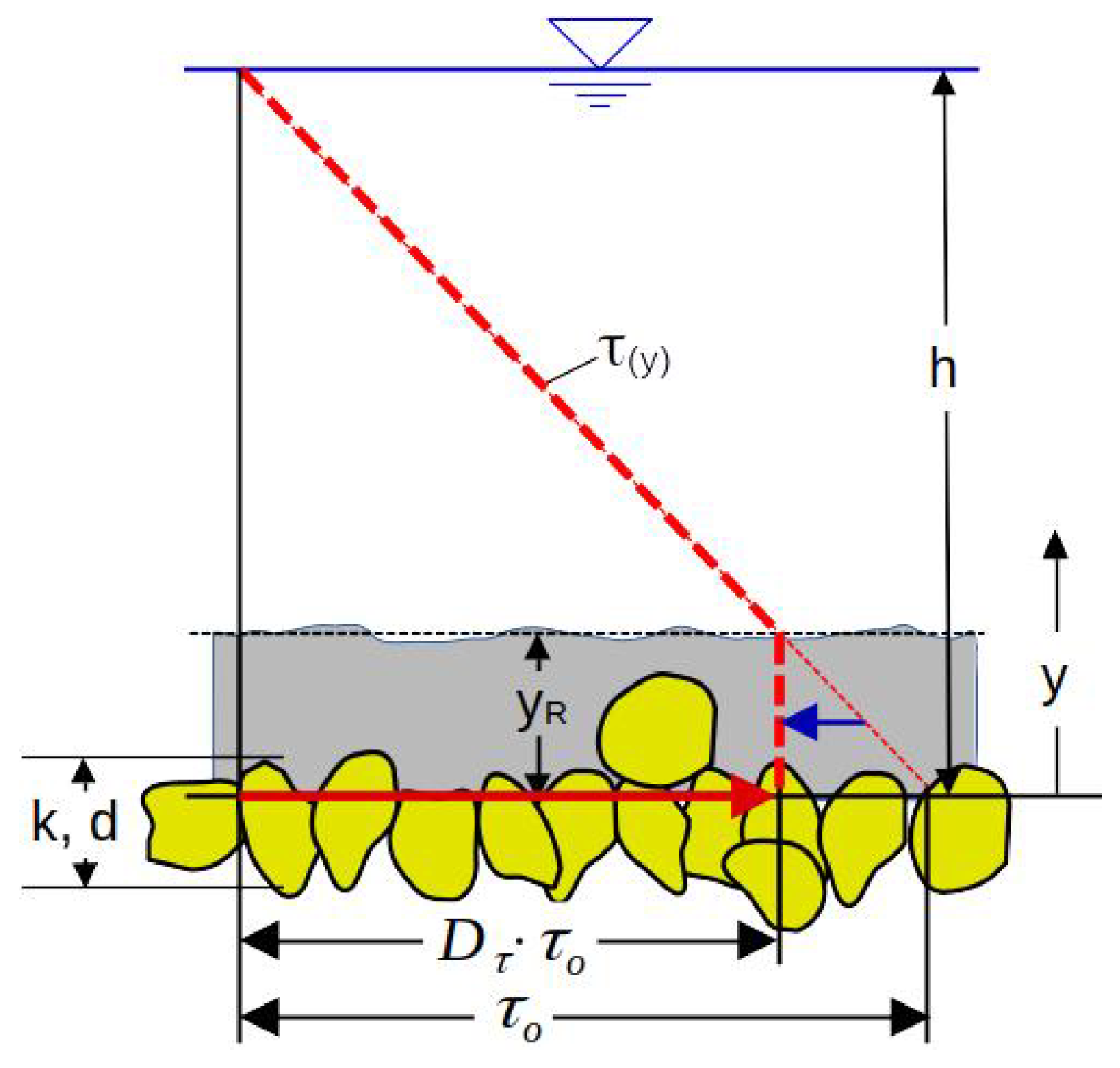
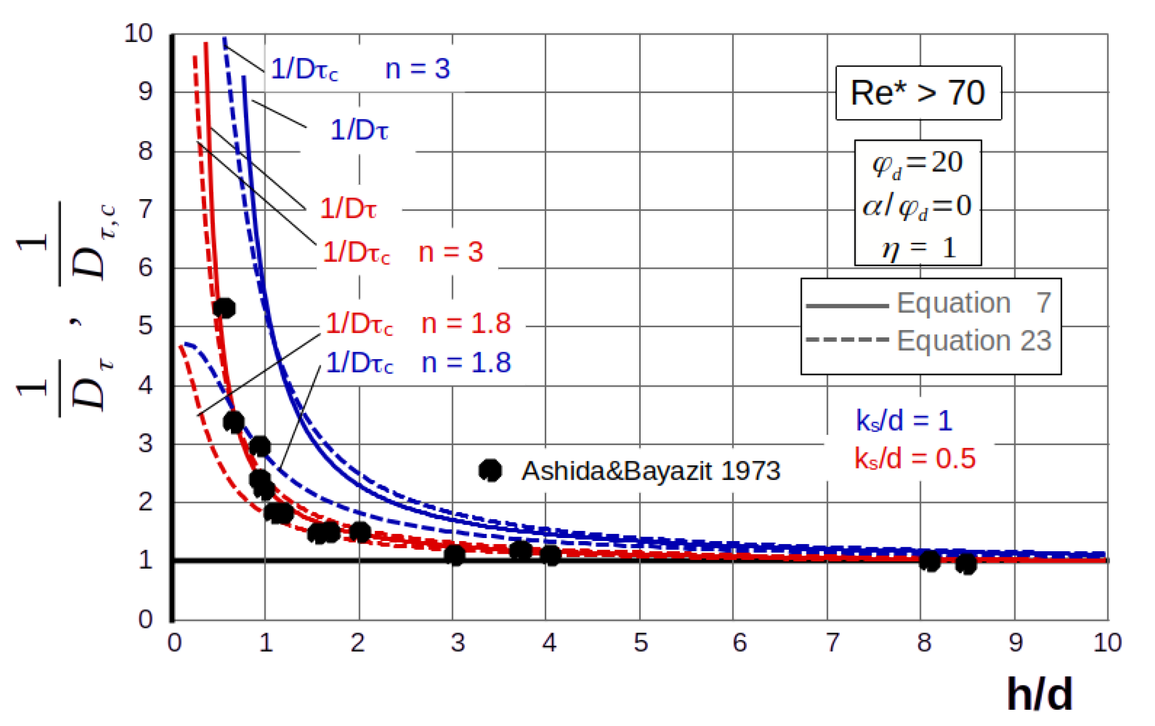
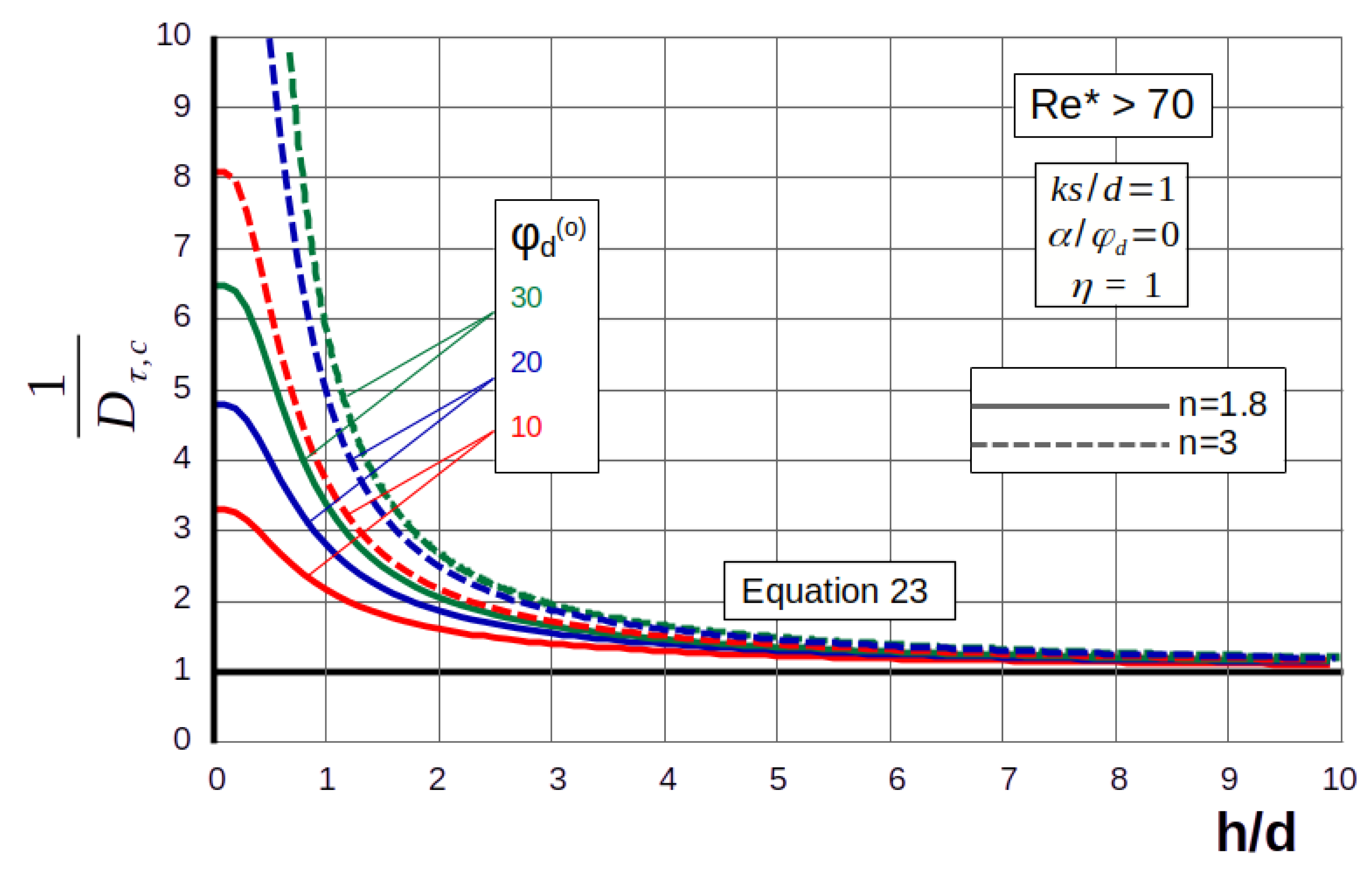
4. Critical Shear Stress at Large Slope and Low Water Cover

While a small coverage reduces the effective shear stress on the bed and, thus, decreases sediment mobility, a bed slope eases sediment mobility (Equation (22)). Figure 13 shows an example of the combined effect of slope and water cover for a relative bed slope of $\alpha =1/2{\phi }_d$. Depending on the combination of slope and water coverage, one or the other effect predominates. In the example shown, both effects neutralize at $h/d\approx 1$.

In reality, the conditions typically are coupled with larger slope values the smaller the coverage is. Figure 14 shows this for the values measured by Ashida and Bayazit (1973) [2] and for those measured by Prancevic et al. (2014) [8,32]. The values are all in the range of $\eta /D_{ta{u}_c}>1$. Thus, the effect of shear stress damping exceeds the effect of slope. The slope values ($\eta$) are also shown. Table 2 shows the related data reported by Ashida and Bayazit (1973) [2].

The effects of the damping of the effective shear stress at low water cover, on the one hand, and the increased gravitational effect at a gradient in the direction of flow are balanced if

$$\frac{\eta }{D_{\tau ,c}}=1$$

(24)

or resolved by the critical angle (${\alpha }_{crit}$) at which Equation (24) is satisfied, resulting in:

$${\alpha }_{crit}=\phi -ASIN\left(D_{\tau ,c}sin\left(\phi \right)\right)$$

(25)

or, with the simplification according to Equation (14) ($\eta \approx 1-\alpha /\phi$):

$$\frac{{\alpha }_{crit}}{\phi }\approx 1-D_{\tau ,c}balanced effect sofslope and coverage$$

(26)

Figure 15 shows the critical angle (${\alpha }_{crit}$) of the bed slope, where the effects of bed slope and low cover balance each other. Only when this angle of bed slope is exceeded do the effects of slope dominate. Thus, under hydraulically rough conditions, e.g., $h/d=5$, the value of $D_{\tau }\approx 0.7$ (see Figure 5). Thus, according to (26), it follows that ${\alpha }_{crit}\approx 0.3{\phi }_d$. Then, when, for example, ${\phi }_d={20}^o$, a slope of $\alpha ⪆6^o$ is required to compensate for the effects of shear stress damping.

5. Influence of Sediment Density

Prancevic and Lamb (2015) [9] investigated not only gravel with ${\rho }^{\prime }=1.65$ but also sediment made of acrylic granules with ${\rho }^{\prime }=0.15$. For this lightweight sediment, the authors found a drastic increase in the shear stress critical for the onset of motion of about three times compared to gravel at about the same slope. That is, $\eta /D_{{\tau }_c}$ was found to be about threefold greater than for the gravel in the experiments. Although no data on internal friction were provided for this sediment and, therefore, the slope parameter ($\eta$) cannot be determined, the slopes in these experiments were comparatively so small that approximately $\eta \approx 1$ applies. Thus, $1/D_{{\tau }_c}$ is also applicable as a comparative value and can be calculated solely from the given values of $h/d$ with Equation (7). The results are shown with those of the other experiments in Table 2 and Figure 16 and are in agreement with the observations.

With approximately the same slope values, they are also about three according to Equation (7), i.e., the solution presented here also covers different sediment densities. It is noteworthy that the sediment densities are not included at all in the solution equation for $\frac{\eta }{D_{\tau }}=\frac{{\tau }_{c,h/d,\alpha }}{{\tau }_{c,\infty ,0}}=\frac{{\tau }_{c,h/d,\alpha }^{★}}{{\tau }_{c,\infty ,0}^{★}}$. This can be explained as follows. At lower sediment densities, the required critical flow velocities are reduced and can be estimated according to Zanke (1977) [42] for low bottom gradients and large water covers with

$$v_{m,c}\approx 2.8\sqrt{{\rho }^{\prime }gd}$$

(27)

In the case of the investigations conducted by Prancevic and Lamb (2015), $\frac{v_{m,c,acrylic}}{v_{m,c,gravel}}=\sqrt{\frac{0.150.023}{1.650.015}}=0.37$. Thus, friction must be increased to produce 0.37 times the velocity at the same slope. This, in turn, requires a reduced relative water depth ($h/d$). Smaller $h/d$ values cause higher turbulence damping; thus, correspondingly higher shear stress is required at the beginning of the movement.

6. Summary and Conclusions

As expected, increased gradients in a downslope flow cause easier mobility of sediments and consequently increased sediment transport. However, a large number of observations have shown the opposite. This paper analyzes the reasons for this and shows how the relative water cover is the reason that the large gradient often does not have the initially expected enhancing effect on sediment movement.

As the result of our research, this is because flows at larger gradients are often associated with shallow water depths, and damping of near-bottom turbulence occurs under low water cover ($h/d$) or large relative roughness ($d/h$) over rough beds. This results in a reduction in the acting shear stresses and explains why, despite the significant slope of the bottom, not smaller but increased shear stresses may be required to move the sediments compared to the case with a smaller slope. The decisive factor is the ratio of slope influence to damping influence on the shear stresses. The mechanical relationships for this are presented herein. For natural conditions, the damping effect of the turbulence near the bottom often outweighs the driving effect of the slope when the sediments start to move.

Finally, it should be mentioned that the effects of low water cover also play a crucial role in the problem of the formation of beach slopes under the uprush and downrush of waves, which has not yet been fully solved. This is because the return water of each wave has the effect of low water cover, especially in coarse sediments.

References

1. Shields, A. Anwendung der Ähnlichkeitsmechanik und der Turbulenzforschung auf die Geschiebebewegung. (Application of Similarity Principles and Turbulence Research to Bed-Load Movement); Mitteilungen der Preussischen Versuchsanstalt für Wasserbau und Schiffbau: Berlin, Germany, 1936; Heft 26. (In German) [Google Scholar]
2. Ashida, K.; Bayazit, M. Initiation of motion and roughness of flows in steep channels. J. Water Resour. Prot. 1973, 3, 475–484. [Google Scholar]
3. Shvidchenko, A.B.; Pender, G. Flume study of the effect of relative depth on the incipient motion of coarse uniform sediments. Water Resour. Res. 2000, 36, 619–628. [Google Scholar] [CrossRef]
4. Gregoretti, C. The initiation of debris flow at high slopes: Experimental results. J. Hydraul. Res. 2000, 38, 83–88. [Google Scholar] [CrossRef]
5. Armanini, A.; Gregoretti, C. Incipient sediment motion at high slopes in uniform flow condition. Water Resour. Res. 2005, 41, 83–114. [Google Scholar] [CrossRef]
6. Lamb, M.P.; Dietrich, W.E.; Venditti, J.G. Is the critical Shields stress for incipient sediment motion dependent on channel-bed slope? J. Geophys. Res. 2008, 113, F02008. [Google Scholar] [CrossRef]
7. Recking, A. Theoretical development on the effects of changing flow hydraulics on incipient bed load motion. Water Resour. Res. 2009, 45, W04401. [Google Scholar] [CrossRef]
8. Prancevic, J.P.; Lamb, M.P.; Fuller, M.F. Incipient motion across the river to debris-flow transition. Geology 2014, 42, 191–194. Available online: https://kiss.caltech.edu/papers/surface/papers/incipient.pdf (accessed on 14 July 2023).
9. Prancevic, J.P.; Lamb, M.P. Unraveling bed slope from relative roughness in initial sediment motion. J. Geophys. Res. Earth Surf. 2015, 120, 474–489. [Google Scholar] [CrossRef]
10. Prancevic, J.; Lamb, M. Particle friction angles in steep mountain channels. J. Geophys. Res. Earth Surf. 2015, 120, 242–259. [Google Scholar] [CrossRef]
11. Zanke, U. Zum Einfluss der Turbulenz auf den Beginn der Sedimentbewegung. (On the Influence of Turbulence on the Initiation of Sediment Motion); Mitt. des Instituts für Wasserbau und Wasserwirtschaft der TU: Darmstadt, German, 2001; Heft 120. (In German) [Google Scholar]
12. Zanke, U. On the influence of turbulence on the initiation of sediment motion. Int. J. Sediment Res. Beijing. 2003, 18, 17–31. [Google Scholar]
13. Nezu, I.; Rodi, W. Open Channel Flow Measurements with a Laser Doppler Anemometer. ASCE J. Hydraul. Eng. 1986, 112, 335–355. [Google Scholar] [CrossRef]
14. Laufer, J. The Structure of Turbulence in Fully Developed Pipe Flow; NACA-Report 1174; National Advisory Committee for Aeronautics: Edwards, CA, USA, 1954.
15. Grass, A.J. Structural features of turbulent flow over smooth and rough boundaries. J. Fluid Mech. 1971, 50, 233–255. [Google Scholar] [CrossRef]
16. Eckelmann, H. The structure of viscous sublayer and the adjacent wall region in a turbulent channel. J. Fluid Mech. 1974, 65, 439–459. [Google Scholar] [CrossRef]
17. Steffler, P.M.; Rajaratnam, N.; Peterson, A.W. LDA measurements in open channel. J. Hyd. Eng. ASCE 1985, 111, 119–130. [Google Scholar] [CrossRef]
18. Nezu, I.; Nakagawa, H. Turbulence in Open Channel Flows. In IAHR Monograph; A. A. Balkema: Rotterdam, The Netherlands, 1993. [Google Scholar]
19. Zanke, U. Hydromechanik der Gerinne und Küstengewässer (Hydromechanics of Flumes and Coastal Waters); Parey-Verlag: Berlin, Germany, 2002. (In German) [Google Scholar]
20. Bezzola, G.R. Fliesswiderstand und Sohlenstabilität Natürlicher Gerinne. (Flow Resistance and Bed Stability of Natural Channels); Mitt. der VAW; ETH: Zuerich, Switzerland, 2002; Heft 173. [Google Scholar]
21. Bayazit, M. Free Surface Flow in a Channel of Large Relative Roughness. JHR 1976, 14, 115–126. [Google Scholar] [CrossRef]
22. Bayazit, M. Flow structure and sediment transport in steep channels. In Proceedings of the Euromech 156 ‘Mechanics of Sediment Transport’, Istanbul, Turkey, 12–14 July 1982; Sumer, M., Müller, A., Eds.; pp. 197–206. [Google Scholar]
23. Rickenmann, D. Fliessgeschwindigkeit in Wildbächen und Gebirgsflüssen (Flow velocity in torrents and mountain rivers). Wasser Energie Luft 1996, 88, 298–304. (In German) [Google Scholar]
24. Ruf, G. Fliessgeschwindigkeiten in der Ruetz/Stubaital, Tirol. (Flow velocities in the Ruetz/Stubaital, Tyrol). Wildbach Lawinenverbau 1990, 115, 219–227. (In German) [Google Scholar]
25. Jarrett, R.D. Hydraulics of high-gradient streams. J. Hyd. Eng. ASCE 1984, 110, 1519–1539. [Google Scholar] [CrossRef]
26. Bathurst, J.C. Flow resistance estimation in mountain rivers. J. Hyd. Eng. ASCE 1985, 111, 625–643. [Google Scholar] [CrossRef]
27. Thompson, S.M.; Campbell, P.L. Hydraulics of a large channel paved with boulders. J. Hyd. Res. 1979, 17, 341–354. [Google Scholar] [CrossRef]
28. Thorne, C.R.; Zevenbergen, L.W. Estimating mean velocity in mountain rivers. J. Hyd. Eng. ASCE 1985, 111, 612–624. [Google Scholar]
29. Griffith, G.A. Flow resistance in coarse gravel bed rivers. J. Hyd. Div. ASCE 1981, 107, 899–918. [Google Scholar] [CrossRef]
30. Raupach, M.R. Conditional statistics of Reynolds stress in rough-wall and smooth-wall turbulent boundary layers. J. Fluid Mech. 1981, 108, 363–382. [Google Scholar] [CrossRef]
31. Lamb, M.P.; Brun, F.; Fuller, M. Hydrodynamics of steep streams with planar coarse-grained beds: Turbulence, flow resistance, and implications for sediment transport. Water Resour. Res. 2017, 53, 2240–2263. [Google Scholar] [CrossRef]
32. Prancevic, J.P.; Lamb, M.P.; Fuller, M.F. Supplementary Materials for: Incipient motion across the river to debris-flow transition. Geology 2014, 43, 191–194. Available online: https://authors.library.caltech.edu/45096/7/2014067.pdf (accessed on 14 July 2023).
33. Zanke, U. The beginning of sediment movement as a probability problem. In Proceedings of the Int. Sympos. Sediment Transport Modeling, New Orleans, LA, USA, 14–18 August 1989. [Google Scholar]
34. Zanke, U. Zum Übergang Hydraulisch glatt - Hydraulisch rauh. (On the transition hydraulically rough-hydraulically smooth). Wasser Boden 1996, 48, 32–36. (In German) [Google Scholar]
35. Zanke, U. Lösungen für das universelle Geschwindigkeitsverteilungsgesetz und die Shields-Kurve. (Solutions for the universal velocity distribution law and the Shields curve). Wasser Boden 1996, 9, 21–26. (In German) [Google Scholar]
36. Reichardt, H. Vollständige Darstellung der turbulenten Geschwindigkeitsverteilung in glatten Leitungen. (Complete representation of the turbulent velocity distribution in smooth pipes). ZAMM Z. Für Angew. Math. Mech. 1951, 31, 208–219. (In German) [Google Scholar] [CrossRef]
37. Zanke, U. Vorlesungsskript ’Sedimenttransport’ (Scriptum ’Sediment Transport’); Institut für Wasserbau und Wasserwirtschaft der TU Darmstadt: Darmstadt, Germany, 2004; (unpublished). [Google Scholar]
38. Zanke, U.; Roland, A. Sediment Bed-Load Transport: A Standardized Notation. Geoscience 2020, 10, 368. [Google Scholar] [CrossRef]
39. Hanes, D.M.; Inman, D.L. Experimental evaluation of a dynamic yield criterion for granular fluid flows. J. Geophys. Res. Solid Earth. 1985, 90, 3670. [Google Scholar] [CrossRef]
40. Madsen, O.S.; Grant, W.D. Mechanics of cohesionless sediment transport in coastal waters. In Coastal Sediments; ASCE: New York, NY, USA, 1991. [Google Scholar]
41. Nino, Y.; Garcia, M. Using Lagrangian particle saltation observations for bedload sediment transport modelling. Hydrol. Process. 1998, 12, 1197–1218. [Google Scholar] [CrossRef]
42. Zanke, U. Neuer Ansatz zur Berechnung des Transportbeginns von Sedimenten unter Strömungseinfluss (New Approach for the Calculation of the Beginning of Sediment Transport under the Influence of Flows); Mitt. des Franzius-Instituts der Univ.: Hannover, Germany, 1977; Heft 46. (In German) [Google Scholar]
Figure 1. v r m s , b / v at bed level for different values of relative coverage ( h / k s ); graphical representation of Equation (2). δ = thickness of viscous boundary layer = 11.63 ν / v . Modified from [19].
Water 15 02976 g001
Figure 2. The same mean shear stress ( τ ¯ ) causes a different effective shear stress ( τ e f f ) depending on the turbulence conditions (modified from Zanke 2001/2003 [11,12]).
Water 15 02976 g002
Figure 3. Solutions of Equation (7) for different values of the parameters k s / d and k s / d 90 .
Water 15 02976 g003
Figure 5. Damping factors of shear stress under low water coverage. Blue curves represent Equation (6) for different values of R e k s = v k s / ν . The bold blue curve ( R e k s > 70 ) results from Equation (6) and Equation (7). The dashed red curve shows the course of Equations (10) and (11) according to Bezzola [20].
Water 15 02976 g005
Figure 6. Schematic representation of the definition of the roughness sublayer according to Bezzola (2002) [20].
Water 15 02976 g006
Figure 7. A higher mean shear stress ( τ ¯ ) is required for the initiation of sediment motion at lower turbulence (modified according to Zanke (2001/2003) [11,12]).
Water 15 02976 g007
Figure 8. Effect of turbulence damping at small relative coverage ( h / d ) as a function of R e calculated with Equation (15). Blue: n = 1.8 ; red: n = 3 .
Water 15 02976 g008
Figure 9. v y / v at different relative wall distances ( y / k s ) as a function of R e y [37,38]. The yellow region marks the transition from viscous to turbulent flow as a function of y + and between hydraulically smooth and rough flow as a function of k s + . Assignment of the curves to the descriptive equations: A = viscous sublayer, v y v = v ν y ; B = solution hydraulically rough, Equation (16) with integration constant B = 8.5 (green curves); C = classical smooth–rough transition approach, Equation (16) with B according to Equation (17) (blue curves); D = continuous solution Equation (20) (red curves).
Water 15 02976 g009
Figure 10. Reduced turbulence damping on protruding particles. The blue arrow shows the damping at the protruding grain. This is lower than at the bed (modified after Bezzola [20]).
Water 15 02976 g010
Figure 11. Influence of k S / d on the effect of turbulence damping on critical shear stress under hydraulically rough conditions. Blue: k S / d = 1 ; red: k S / d = 0.5 . Data reported by Ashida and Bayazit (1973) [2] were adjusted for the influence of bed slope. (Note that Equation (23) for h / d 0 goes against a finite value, unlike Equation (7)).
Water 15 02976 g011
Figure 12. Effect of φ d on D τ , c according to Equation (23) presented for φ d = 10 , 20 , 30 for n = 1.8 (corresponding to a motion state like the Shields curve) and for n = 3 (corresponding to start of motion of separated grains).
Water 15 02976 g012
Figure 13. Example of the influence of slope and shear stress damping on the critical shear stress under hydraulically rough conditions. In the range of η / D τ , c < 1 , the slope effect is dominant. At η / D τ , c = 1 , (in this example) the effects of slope and turbulence damping cancel each other out, and at η / D τ , c > 1 , the effect of turbulence damping predominates (Equation (7), with k S / d = 0.5 ).
Water 15 02976 g013
Figure 14. Increase in critical shear stress according to experiments conducted by Ashida and Bayazit (1973) [2] and by Prancevic et al. (2014) [8,32] in comparison with calculated values. In all cases, the influence of turbulence damping overcomes the influence of slope ( D τ c < η ). Also shown are the values of η associated with the individual measured values.
Water 15 02976 g014
Figure 15. Some examples for critical bed slopes where the effects of slope (increasing sediment mobility) and the effects of low water coverage (decreasing sediment mobility) are balanced. In the case of R e > 70 based on Equation (6) or (7) and in the case of R e = 10 based on Equation (23), lower R e lower near bed turbulence → lower turbulence damping → smaller effect of h / d .
Water 15 02976 g015
Figure 16. Critical shear stress ( τ c , h / d , α 1 / D τ c ) as a function of slope. The values for the acrylic sediment reported by Prancevic and Lamb (2015) obtained relative to gravel using Equation (7) increased by about three times for the same slope, as also observed by in the present study. Data by Ashida & Bayazit [2], Prancevic, Lamb & Fuller [8], Prancevic & Lamb [9,10].
Water 15 02976 g016