Article

Multi-Dimensional Surface Water Quality Analyses in the Manawatu River Catchment, New Zealand

1
Mineta Transportation Institute, San Jose State University, San Jose, CA 95192, USA
2
Department of Geography and Environmental Studies, Texas State University, San Marcos, TX 78666, USA
3
Department of Civil Engineering, Covenant University, Ota 112104, Nigeria
4
Albert B. Alkek Library, Texas State University, San Marcos, TX 78666, USA
5
Department of Physics, Covenant University, Ota 112104, Nigeria
6
Department of Chemical Engineering, Covenant University, Ota 112104, Nigeria
7
Civil Engineering Program, Ingram School of Engineering, Texas State University, San Marcos, TX 78666, USA
8
Politechnical School, Unisinos University, Sao Leopoldo 93022-750, Brazil
*
Author to whom correspondence should be addressed.
Water 2023, 15(16), 2939; https://doi.org/10.3390/w15162939
Submission received: 19 June 2023 / Revised: 4 August 2023 / Accepted: 9 August 2023 / Published: 15 August 2023
(This article belongs to the Special Issue Water Quality, Water Security and Risk Assessment)

Abstract

:
Land Use and Land Cover (LULC) properties give vital information about pollution signatures in rivers, and they help develop best management practices (BMPs) for effective water resource management. This work employs multivariate statistical methods, receptor modeling, connectivity analysis, and univariate trend analysis to investigate pollution sources across spatiotemporal scales in the Manawatu River, New Zealand. A positive matrix factorization (PMF) method was applied to interpret possible contamination sources. A 25-year dataset (1989–2014) comprising 12 water quality variables from three sites was used. Runoff connectivity analyses identified high-producing grassland (HG) as the most dominant pollution class in all sub-catchments. Univariate analyses revealed that nutrients and sediments were higher than in the initial monitoring years. The PMF analysis found possible pollutants causing impairment, which required attention from waste managers. PMF also showed that point, natural, and agricultural sources significantly contributed to pollution downstream of the river. In the midstream, the erosion, point, and agricultural sources were significant contributing factors. Agricultural pollution and soil erosion were the main contributors to the upstream sub-catchment area. This study suggests that BMPs with a high retention capacity are needed in specific locations in the catchment area to filter high concentrations of pollutants generated.

1. Introduction

Clean water is vital for many daily activities and good health [1,2]. However, with advances in agricultural, industrial, and urban development, maintaining water quality at preferred standards has been difficult in recent times [3,4,5,6]. The quality of water sources, particularly surface water, is the sum of the components of the surrounding watershed, with land-use activities identified as being responsible for the impairment of water quality [7,8]. One of the main reasons is that land use decisions are made without considering the watershed’s assimilatory capacity [9,10]. The authors in a recent publication [11] found that an excess influx of nutrients beyond the river’s assimilation capacity results in poor water quality.
When water quality is adversely affected, ecosystem function is disrupted. The consequences are eutrophication or sedimentation [12]. For example, phosphorus and nitrogen from fertilizer in agricultural areas have been major causes of pollution, leading to algal blooms in rivers and lakes. These impairments can reduce the aesthetic quality of the river due to a reduction in clarity [13], and they can reduce oxygen levels when dead zones are created. Changes in the levels of other variables, such as dissolved oxygen, temperature, pH, and total suspended solids, can affect ecosystem performance, especially when they fall out of the recommended ranges. Thus, it is crucial to monitor water quality, reduce soil erosion, and prevent runoff entering water bodies to ensure they are maintained at an acceptable standard. The implementation of a wide range of watershed best management practices (BMPs) has been suggested in the literature. These include waste stabilization ponds, wetlands, animal fencing, and riparian restoration [14]. Riparian restoration has proven to be the preferred method of policy makers, as it can be a cost-effective option when installed in an appropriate location within a river catchment.
In the absence of riparian restoration, a consistent water quality assessment is required to determine the state of the water bodies. This assessment will assist watershed managers in developing optimal policies, decisions, and management practices. Water quality assessments can be performed using routinely monitored stations. These stations enable relevant authorities to gather data that can be analyzed using univariate and multivariate statistical methods. These methods have been applied collectively to detect potential sources of pollution and the relationships between variables in clusters. However, performing these analyses in isolation may lead to incorrect conclusions. Several studies in the literature have utilized these techniques to propose cause-and-effect relationships between environmental pollution associated with groundwater [15,16,17,18] and surface water [19].
New Zealand (NZ) has been identified as a nation that experiences surface water quality problems that are associated with intensive land use [20,21,22]. Certainly, New Zealand stands as a significant global exporter of sheep products, powdered milk, and butter. This surface water quality issue can be linked to the nation’s heightened level of agricultural productivity [23]. This dominance in agriculture is likely to stress river water quality, as more fertilizers are required to increase agricultural production. NZ began consistently collecting and monitoring water quality data on a national scale in 1989 [24]. As reported in Davies-Colley et al. [25], their National River Water Quality Network (NRWQN) has been in operation for three decades, and it has consistently monitored water quality variables. This robust dataset encompasses the spatial and temporal variability of water quality. Seventy-seven sites were monitored throughout thirty-five rivers across NZ, with each site close to a hydrometric station. Although several studies have used this dataset to reveal water quality issues on a national scale [21,26,27,28,29,30], very few have used it to identify sources of pollution on regional and catchment scales.
As water quality issues are location-dependent, they are influenced by natural processes and anthropogenic activities in the watershed. This study applied multivariate statistical analyses to determine the seasonal and spatial patterns of water quality impairments in the Manawatu River. Additionally, this study assessed the overall state of the watershed in terms of pollutant concentrations by apportioning sources using a receptor modeling technique. Finally, we compared our water quality findings with runoff connectivity and land use/land cover (LULC) data to identify specific landscape connections and contributions. This multi-dimensional analysis can be used to inform water-management strategies.

2. Materials and Methods

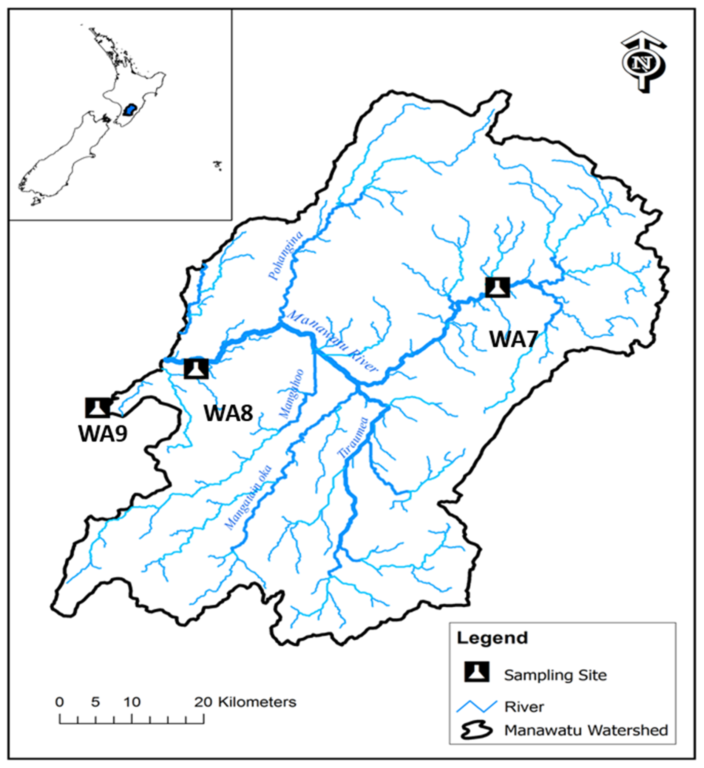
2.1. Study Area Physical Geography

The 5879 km2 Manawatu catchment is situated on the southern tip of the North Island of NZ (Figure 1). Within this watershed, three NRWQN monitoring stations have been used to collect water quality variables since 1989. The first station in the upstream section was mainly surrounded by grassland and pasture, whereas the midstream station was adjacent to large built-up areas. The last station was situated near the catchment outlet. Larned et al. [27] and Abott et al. [31] reported that the Manawatu River is affected by sediment primarily because of intensive land use on moderate to steep slopes comprising erodible soils. The southern and eastern regions of the Manawatu catchment are mountainous and hilly, respectively, and they are covered by natural forests and shrublands, some of which have been converted to pastures for beef cattle, dairy, and sheep farming [14]. It is situated on soft sedimentary rocks that are characterized by mudstone and sandstones. The mountains contain hard, dark grey-brown soils that produce fine deposits when eroded, whereas the hills are characterized by tertiary-aged mudstone or sandstone [14]. Substantial amounts of sediment from this catchment (proliferated by land clearing) are generated in the ocean at a rate of Ca 3.74 Mt yr−1 [32].
In accordance with Land Air Water Aotearoa [33], the Manawatu River is 235 km long. It has several large tributaries, such as the Mangahoo, Mangatain oka, Oroua, Pohangina, and Tiraumea rivers, which are 86, 71, 131, 71, and 69 km, respectively. The river starts in the eastern part of NZ and gradually moves into the Tasman Sea. Land use in the Manawatu catchment predominantly consists of agricultural activities (70%). Half of the agricultural land is used for sheep and beef farming [33]. Within the catchment, Palmerston North, where the WA8 sampling site is situated, had the largest urban settlement. In addition, there are numerous other small communities within the catchment. The settlers in these communities practice intensive agriculture and have done so for years, which suggests that the primary consumptive use of the river within the catchment is for irrigation purposes.

2.2. Water Quality

The Manawatu catchment is located within the Manawatu–Wanganui region, which has some distinctive topography, including the Ruahine, Tararua, and Puketoi Ranges. These ranges exceed 1000 m in terms of elevation, but they drop to form a ridge as they approach the Manawatu gorge. Water quality data were collected monthly by the National Institute for Water and Atmospheric Research (NIWA) from three monitoring sites within the Manawatu catchment for 25 consecutive years (1989–2014). These three stations comprised a longitudinal study, cutting across the upland river with an altitude of >150 m, and they were assumed to be less polluted (WA7) than the lowland (lower elevation) river with an altitude of <150 m. These lowland rivers will likely witness higher background concentrations as the accumulated diffuse pollution flows downstream (WA8 and WA9). A summary of different site characteristics is presented in Table 1. More specifically, WA7 (Manawatu at Weber Road) is in the upstream section of the Manawatu catchment, with a median temperature of 13 °C and a catchment area of 705 km2. WA8 (Manawatu at Teachers College) was located at an intermediate point.
The catchment area of WA8 encompasses 3897 km2, and it is located in the center of Palmerston North. It has experienced significant soil erosion, which has affected the river’s water quality owing to its low elevation, as compared with WA7. It consists of major rivers with significant pastoral development, and it has a median temperature of 13.8 °C. WA9 (Manawatu at Opiki Bridge) is located in the downstream section of the river. This catchment has a median temperature of 14.4 °C, and it receives treatment for industrial and sewage discharges.
The dataset used for this study included data collected from the inception of the water quality monitoring program, which was established by the NRWQN between Jan 1989 and Dec 2014, considering 12 variables (Table 2). Of the 12 parameters measured, five were measured in situ, and seven others were measured in the laboratory. The water quality variables measured in the field were Discharge (Q), Dissolved Oxygen (DO), Water Clarity (CLAR), turbidity (TURB), and Water Temperature (Tw). Moreover, pH, Total Phosphorus (TP), Total Nitrogen (TN), Dissolved Reactive Phosphorus (DRP), Oxidized Nitrogen (NOx), Colored Dissolved Organic Matter (CDOM), and Conductivity (COND) were measured in the laboratory [24]. Smith and McBride [24] and Davies-Colley et al. [34] provided detailed accounts of how the water samples were collected. At the beginning of the sampling years, and up until 2004, samples taken for laboratory testing were simultaneously collected in 2 L High-Density polyethylene (HDPE) bottles at each site. In 2005, sampling with 2 L HDPB was replaced with a single 500 mL HDPB of the same quality, and it was produced by the same manufacturer. Water samples were stored in an insulated bin filled with slush ice, and they were immediately transported to a water quality center in Hamilton, New Zealand. These samples were transported immediately to ensure that both chemical and biological tests were conducted within 24 h, in accordance with laboratory standards.

2.3. Statistical Analysis

To determine the quality of the monitored river over time, and to measure average changes in water quality, we grouped the dataset into 5 year periods from 1989 to 2014, except for 1994, which was exempted for all variables due to contamination with ammoniacal nitrogen (NH4+) [34]. This study used median values, rather than mean values, to compare and monitor water quality changes; this is because the latter is sensitive to spread and to extreme values. Median values for each 5 year period were calculated and compared in order to trigger values prepared by Australia and New Zealand for water quality assessments; these values varied between the lowlands and uplands (distinguished in accordance with the 150 m elevation threshold) (Table 2) depending on where the sampling stations were situated (Australian and New Zealand Environment and Conservation Council; ANZECC [35]). These triggered values do not necessarily suggest an immediate threat, but they are a warning sign for future risk if not curtailed. Statistical testing procedures were performed using the SPSS package (V.23) and an R package (R Core Team, 2020), whereas receptor modeling was performed using EPA PMF 5.0 [36]. Before statistical testing and modeling were conducted, missing data were excluded from the analyses. After that, a normality test was performed using the Kolmogorov–Smirnov (K–S) test to determine the distribution of the dataset. This normality test was crucial for identifying the appropriate statistical test to implement the forward movement. For example, a normality test showing a non-normal distribution is usually analyzed using non-parametric statistical methods. In this study, the normality test showed that the dataset was not normally distributed (p < 0.05), except for one or two parameters at some sites. Seasonal pollution patterns were investigated for each site by stratifying the datasets into seasons to determine which season might be an apparent contributor to river water quality compared with the overall pollution status, especially the trigger values.
According to Abott et al. [31], the Manawatu Catchment has two different seasons (summer—November to May; and winter—June to October). Summer, winter, overall, and trigger comparison observations were conducted for both seasons to identify the contribution of seasonality to the water quality variables measured at different sites. A two-tailed, non-parametric Spearman’s correlation test was applied to determine the relationship between the variables (α = 0.05 and 0.01). Spearman correlation coefficient values were reported using the raw data because there was no change in statistical significance central to this study. This study focused on direction and statistically, and the significant difference developed by the variable rather than the coefficient, which was consistent when the transformed Pearson’s correlation coefficient was used [37,38,39,40]. In addition, there were several significant relationships at the 95% and 99% confidence intervals, although many seemed weak. To reduce the number of relationships observed, only Spearman correlation values of (r) > 0.75 were reported.
The positive matrix factorization (PMF) method is used on environmental datasets to identify potential sources and to apportion possible weights in percentages of pollution parameters. This outcome was achieved by decomposing a large temporal dataset into single quantified weights in the form of factor contributions, factor profiles, or factor fingerprints. These factor profiles were sub-divided into concentrations of species (pollutants and their respective percentages). The percentages of these factor profiles were then interpreted as the pollutant prevalence at the sites under investigation. The PMF model can be expressed in the following general form:
X = GF + E
The X matrix was decomposed into G and F matrices, where G represents the factor contribution, and F represents the factor profiles. Matrix E is the residual error, which should be minimized. Minimizing these errors in each variable, such that they tend toward zero, would almost guarantee that the dataset or variable was from a normal distribution. The PMF model generates covariance and correlation matrices to be decomposed, with one of its strengths being the generation of non-negative factors [41]. For this study, the dataset was cleaned to ensure no missing data. In the event of missing data, it was replaced with the median value of a specific variable. The file that is subjected to PMF modeling is called the concentration file. After that, an uncertainty concentration file is created. This refers to the minimum values that a measuring device can record; below this value, no readings can be obtained. The use of an uncertainty dataset in modeling is essential in pollution studies and risk assessment because of the presence of unknown processes or activities, such as experimental precision, instrumental errors, environmental instability effects (climate nonstationarity), and seasonal variability. This phenomenon may affect the output, as well as the corresponding decisions made when neglected, as the model results might have been significantly underestimated. The process of mathematically handling uncertain data files using the PMF approach has been well documented elsewhere [36].
The Uncertainty concentration is obtained, as follows:
=√ ((Error fraction × concentration)2 + (0.5 × MDL)2)
where MDL is the minimum detection limit.
When performing the PMF analysis for this study, all datasets entered showed a strong S/N ratio. This was attributed to the consistency of the data recorded, fewer missing values, and the large dataset or sample size used for the analysis (Table 2). Despite this, some variables were excluded from the analysis because the study focused on variables directly involved in pollution, without including strongly correlated variables that could replace one another. Therefore, temperature, DO, CLAR, and pH were classified as “bad weight”, and the program neglected those variables during computation. However, a “normal”, “bad”, “weak”, or “strong” weight was given to datasets with large, average, and minimum missing values to alert the software program. In this study, all the variables were allocated or described as strong by default. Regression plots showing the corresponding R-squared values for each water quality variable were obtained.

2.4. Land Use Land Cover (LULC) Mapping

A map depicting the existing LULC in the Manawatu catchment was developed to determine the contribution of LULC activity to water quality. Land cover specifies the identifiable features of the land, including the presence of crops, forest plantations, or scrub-grassland covers [11]. Identifying various LULCs is essential as it helps to provide some insight into the sources of diffused pollution within a catchment. LULC data obtained from the land cover database (LCDB v4.1, 2015) were used for this purpose. Thirty-five land use classes were obtained. Moreover, they showed identical and conflicting classifications with the land use and carbon analysis system (LUCAS) data operated by the NZ Ministry for the Environment. Julian et al. [21] detailed these differences and reclassified the LULC to be suitable for effectively establishing a water quality impairment relationship. This study followed the same procedure as [21] to ensure consistency in terms of reporting in accordance with the authors’ detailed output2.5. Landscape Connectivity Analysis
This study used an existing watershed connectivity model, developed by [42], to connect the river to pollution source areas. This map showed that the LULC was directly related to the river via surface runoff. This model was carefully developed following the detailed procedure reported in [43]. The stream channels headed for the Manawatu catchment were identified using 0.5 m rural aerial photos obtained from Land Information, New Zealand, using two-year period data (2010–2012) as the reference point. The watershed was then delineated from the headwaters of the catchment to establish the flow direction, from upstream to downstream. Each 15 m pixel on the digital elevation model, with a greater than 5° slope, along the flow direction, as well as pixels adjacent to the river, were categorized as “connected”. With the landscape connectivity map (Figure 2) developed, it was clipped, combined, and reclassified to select catchments connected to floodplains in the Manawatu catchment area.

3. Results

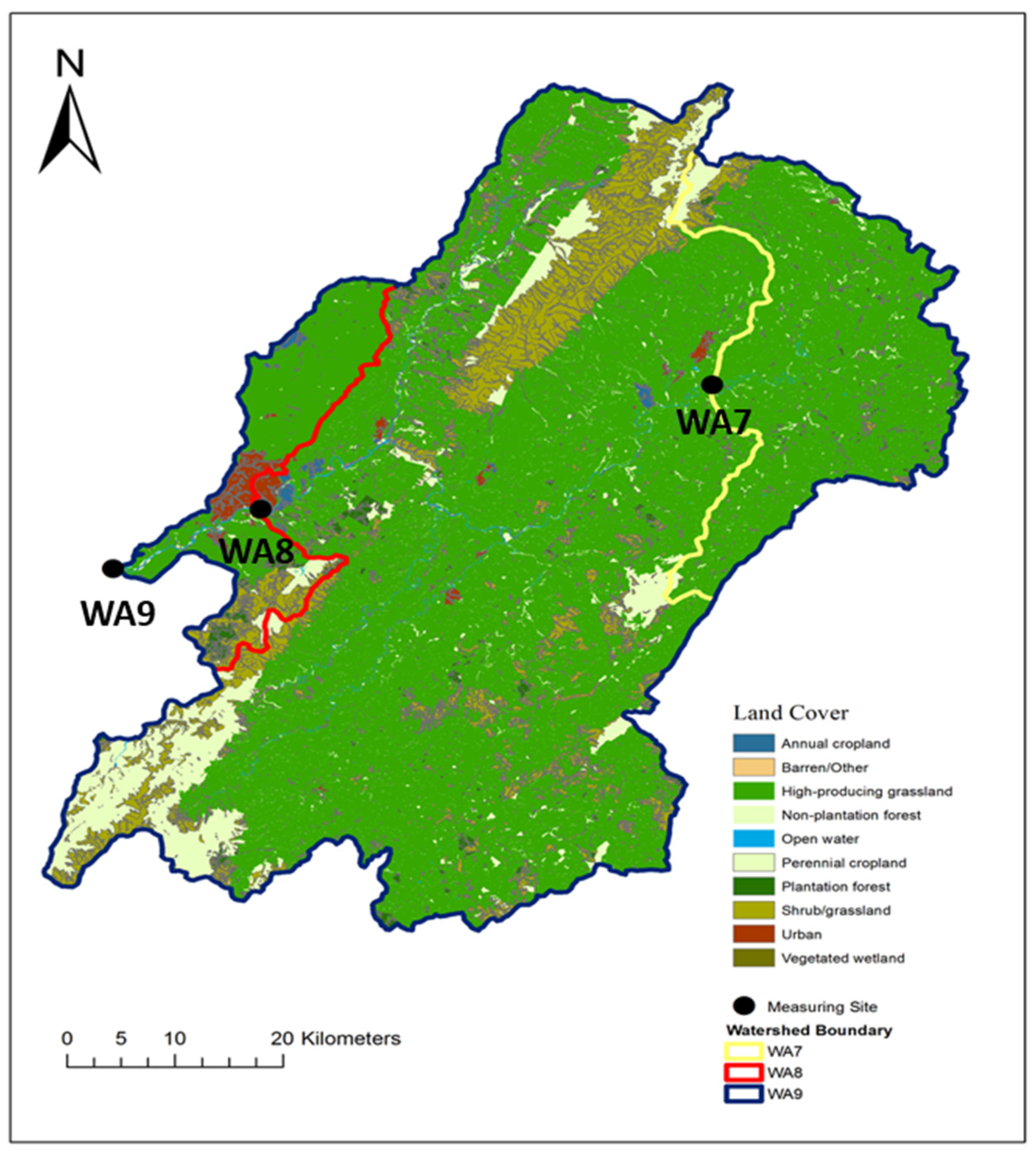
3.1. Land Use Map and Analysis

From LULC mapping (Figure 3), different LULC categories were observed at the three sites within the Manawatu catchment. Eight classes were present in the upstream area, as follows (WA7): shrub/grassland (SG), urban (UR), non-plantation forest (NF), plantation forest (PF), vegetated wetland (VW), high-producing grassland (HG), open water (OW), and barren/other (BO). These categories revealed that perennial and annual croplands did not exist upstream. The catchment of WA7 is dominated by HG (88.5%), NF (3.4%), and PF (3%). For the intermediate site (WA8), all ten LULC categories were obtained. This catchment is dominated by HG (74.1%), SG (14.2%), and NF (8%). The entire Manawatu catchment (WA9; most downstream station) was dominated by HG (74.5%), SG (10.8%), and NF (7.8%).

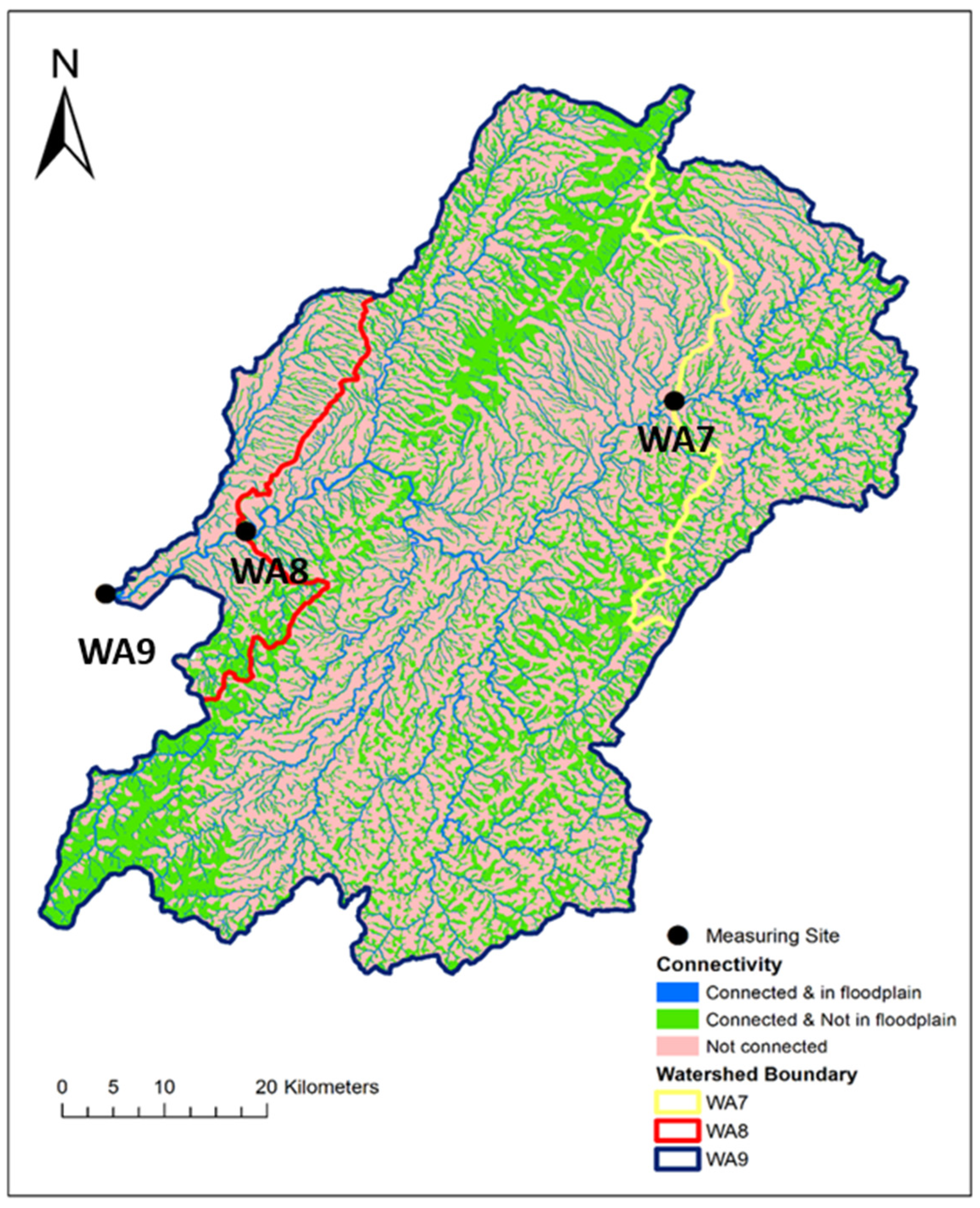
3.2. Landscape Connectivity

Landscape connectivity analyses (Table 3) revealed that 83.6 km2 of the WA7 catchment (or 11.9%) was directly connected to streams via surface runoff and floodplains. Another 196 km2 (27.8%) was related to streams via surface runoff, but not floodplains. That is, these were steep hillslopes that directly contributed to the surface runoff to streams. In total, For WA7′s catchment, 39.7% of the area was directly connected to streams via surface runoff. Approximately 426 km2, more than half of the catchment area, is not directly connected, and it contributes surface runoff to the Manawatu River. HG (88%) was mainly related to a floodplain, which suggests a significant pollution source from the upstream section of the Manawatu River. For the intermediate site (WA8), landscape connectivity results suggest that ~2191 km2 of a total of 3897 km2 of the WA8 catchment (or 56.2%) was not directly connected to the river (Table 3). However, 11.3% of the total area in the WA8 catchment (or 440.9 km2) was directly related to the stream via surface runoff and located in floodplains. Moreover, 32.5% of WA8′s catchment (or 1265.3 km2) was directly connected to a stream via surface runoff and not located in a floodplain. Of note, HG (75.3%) dominated a substantial portion of the area connected to the floodplain, and ~64% of HG (HG area connected and HG not connected to floodplains but connected to catchment) contributed to the Manawatu River. Therefore, for WA8, 43.8% of the catchment area was connected to streams via surface runoff. Regarding the downstream sub-catchment (WA9), 483.9 km2 of the catchment (or 11.5%) was directly connected to the stream via surface runoff and were in floodplains. Another 1343.6 km2 of WA9′s catchment area (or 31.8%) was directly connected to the stream via surface runoff, but not located in floodplains, and 2395.29 km2 (or 56.7%) was not directly connected to either floodplains or the stream via surface runoff (Table 3). Similarly, HG (66%) was the dominant LC in all three sub-catchments.
A comparison was made with their corresponding trigger values to determine the extent to which the water quality parameters were affected by watershed activities, as stipulated by ANZECC [35].

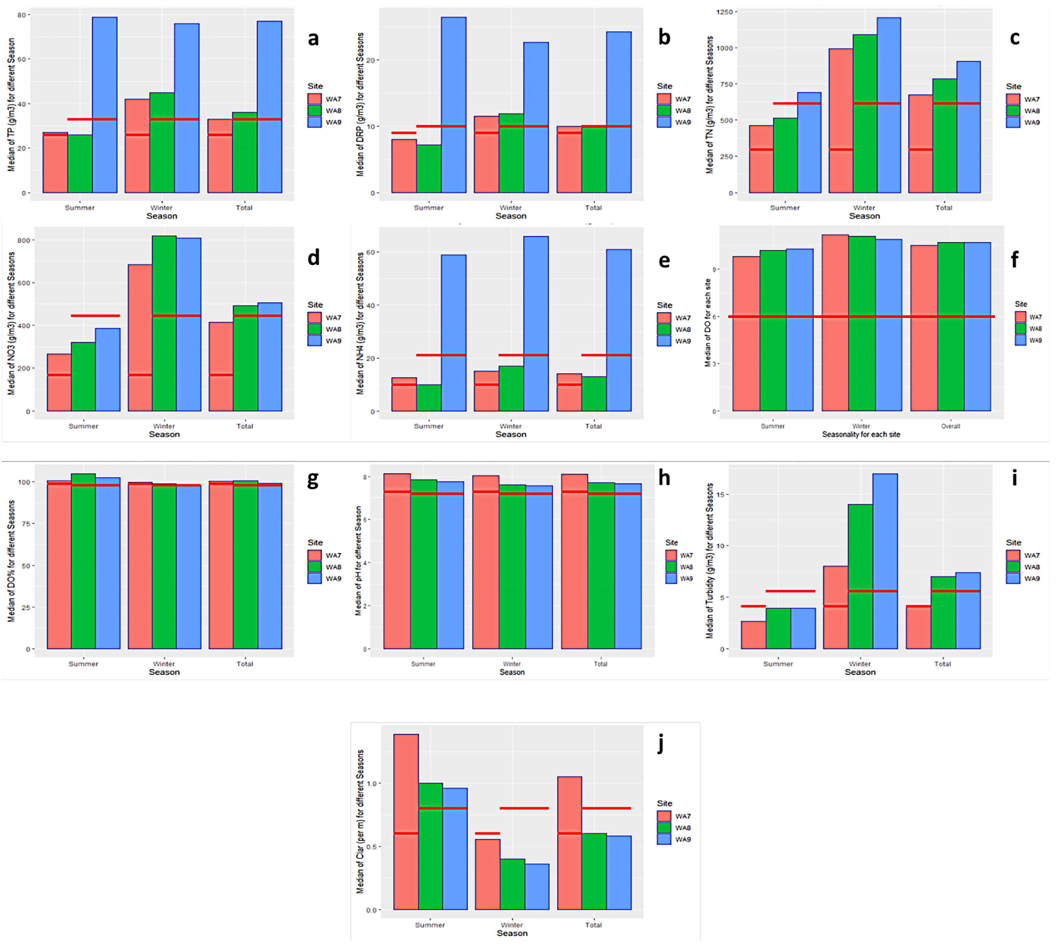
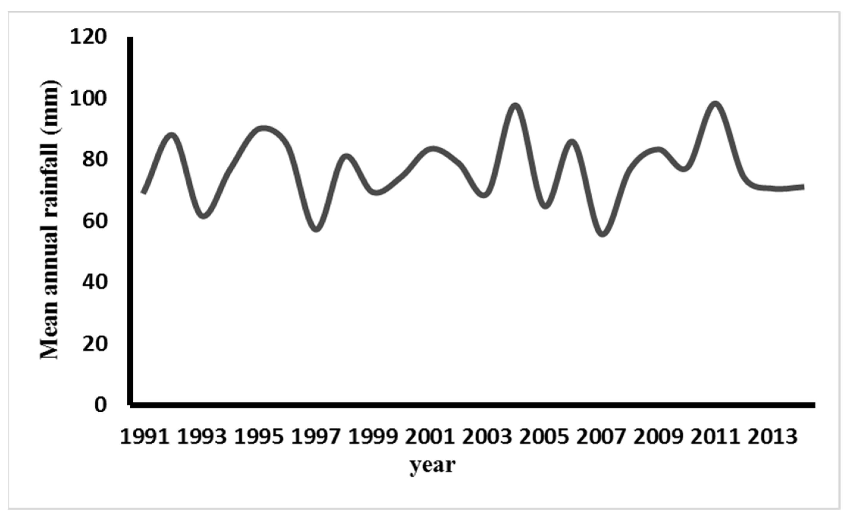
3.3. Seasonality and Trends in Water Quality in the Manawatu Catchment

The TP values (Figure 4a) for WA7 recorded an increasing trend for the first 15 years of sampling and a reduction for the last ten years during the monitoring period. However, the values recorded during this period exceeded the trigger values of 33 g/m3, except for the first and last five years. The lowest median value measured in the first five years of sampling was initially lower than the trigger value, but it later increased between 2000 and 2004. For WA8 (Figure 4a), a similar trend was observed, with a minor difference observed in the first and last five years. The first five years had slightly higher median values than the trigger values, whereas the values during the previous five-year period were lower than the trigger values. This difference may be due to non-point source pollution at WA7 (upland river), which flowed into lowland rivers (WA8 and WA9), as well as the increase in connected pasture areas connected to the floodplain in WA9, compared with WA7. However, this was not the case for WA9. Until 2014, the TP values recorded were higher than the trigger values (Figure 4a). The higher TP values recorded may result from the accumulation of pollutants as they flow downstream. The seasonality comparison for all sites revealed similar trends for WA7 and WA8 (Figure 5a). The TP values in WA7 and WA8 were higher in winter than in summer, whereas the overall median values for both sites were higher than those of the stipulated trigger values. For WA9, which was not the case in summer and winter, the overall median values were higher than the trigger values (Figure 5a).
Throughout the monitoring period, the DRP values were higher than the trigger values for WA9, measuring 9 g/m3 (Figure 4b). Between 1989 and 1993, and 2005 and 2009, there was a reduction in DRP; their levels were lower than the trigger values in WA7 and WA8. These values increased in 2014 and were higher than trigger values. Seasonality comparisons for all sites showed that seasonal values were higher than trigger values for WA9 (Figure 5b). At the same time, the same was only observed for winter and overall median values in WA7 and WA8. As for TN, all three sites (WA7, WA8, and WA9) (Figure 4c) showed similar distribution patterns to the patterns mentioned above from the beginning. The TN values recorded were above the trigger value of 295 g/m3 until 2014. Interestingly, these values were significantly higher between 2000 and 2004. Seasonality across sites revealed that the summer, winter, and overall TN values exceeded the trigger values for all sites (Figure 5c). For NO3, the values recorded throughout all periods were higher than the trigger values for all three sites (Figure 4d). High values above the trigger value of 167 g/m3 were measured during the winter and summer periods (Figure 5d). For NH4+, all the site concentration values monitored over the 25 year period showed that the trigger values of 10 g/m3 were exceeded to different extents (Figure 4e). More specifically, the NH4+ values recorded in WA9 were much higher than those at the other sites. Seasonality values also showed similar observations, with winter, summer, and overall median values exceeding the stipulated trigger values (Figure 5e). All sites (WA7, WA8, and WA9) had DO values below the threshold. Throughout all seasons, the data revealed that despite the number of pollutants entering the river, or that were already present in the river, the DO values were significantly above the trigger values of 6 g/m3 (Figure 4f). The seasonal comparison also corroborates this finding. The functional reaeration capacity of the river allows for more oxygen to be re-introduced when used up, owing to the bathymetry of the river (Figure 5f). Additionally, observation of DO% revealed that all measured values were above the trigger values of 99% for the different sites during all study periods (Figure 4g). The same was observed for the median values, as seasonality was also observed (Figure 5g). The PH values were expected to be above the stipulated trigger value of 7.3. The values recorded during the monitoring periods for the three sites revealed that the median pH values were below the trigger values (Figure 4h). The same was observed during seasonality comparisons, thus corroborating a significant concern regarding high pH values (Figure 5h). For turbidity, WA8 and WA9 (Figure 4i) exhibited similar trends. Initially, the recorded values were below the trigger values, but these values increased over time to be above the trigger value. Nevertheless, in WA7 (Figure 4i), a slightly different pattern was observed. Slightly elevated values were recently recorded, whereas elevated values were measured between 1994 and 1999, and 2000 and 2004, with the highest value recorded between 2000 and 2004. Seasonality analysis revealed that the overall median and winter turbidity values exceeded the trigger values (Figure 5i). WA7 had good overall water clarity compared with WA8 and WA9 (Figure 4j). The water clarity values measured in WA7 exceeded the expectations of trigger values, whereas WA8 and WA9 had poor water clarity and did not meet expectations, except for the values measured in WA8 between 2010 and 2014. The seasonality comparison showed that most of the exceeded values were measured during the summer (Figure 5j), whereas the winter period had poor water quality for all three sites.

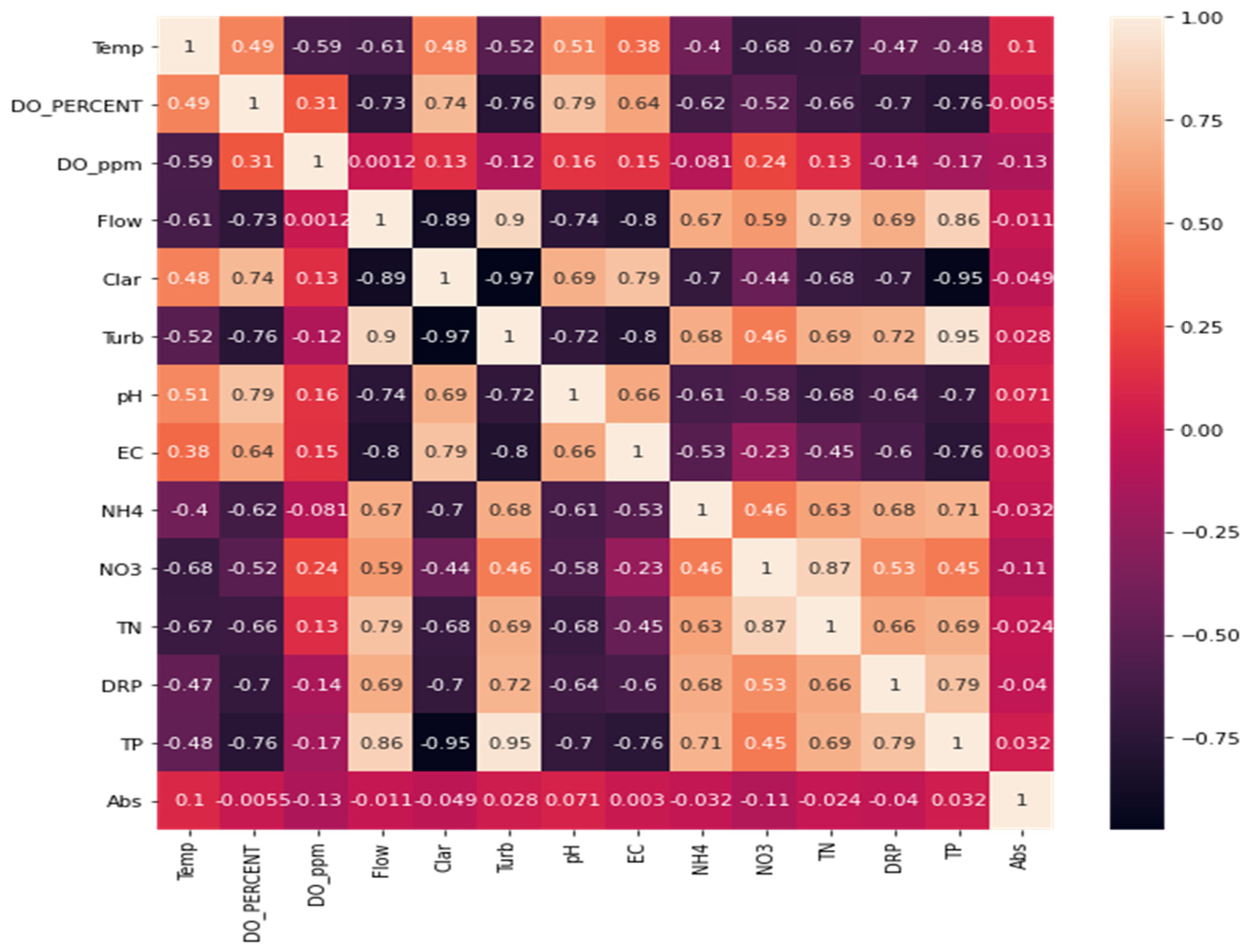
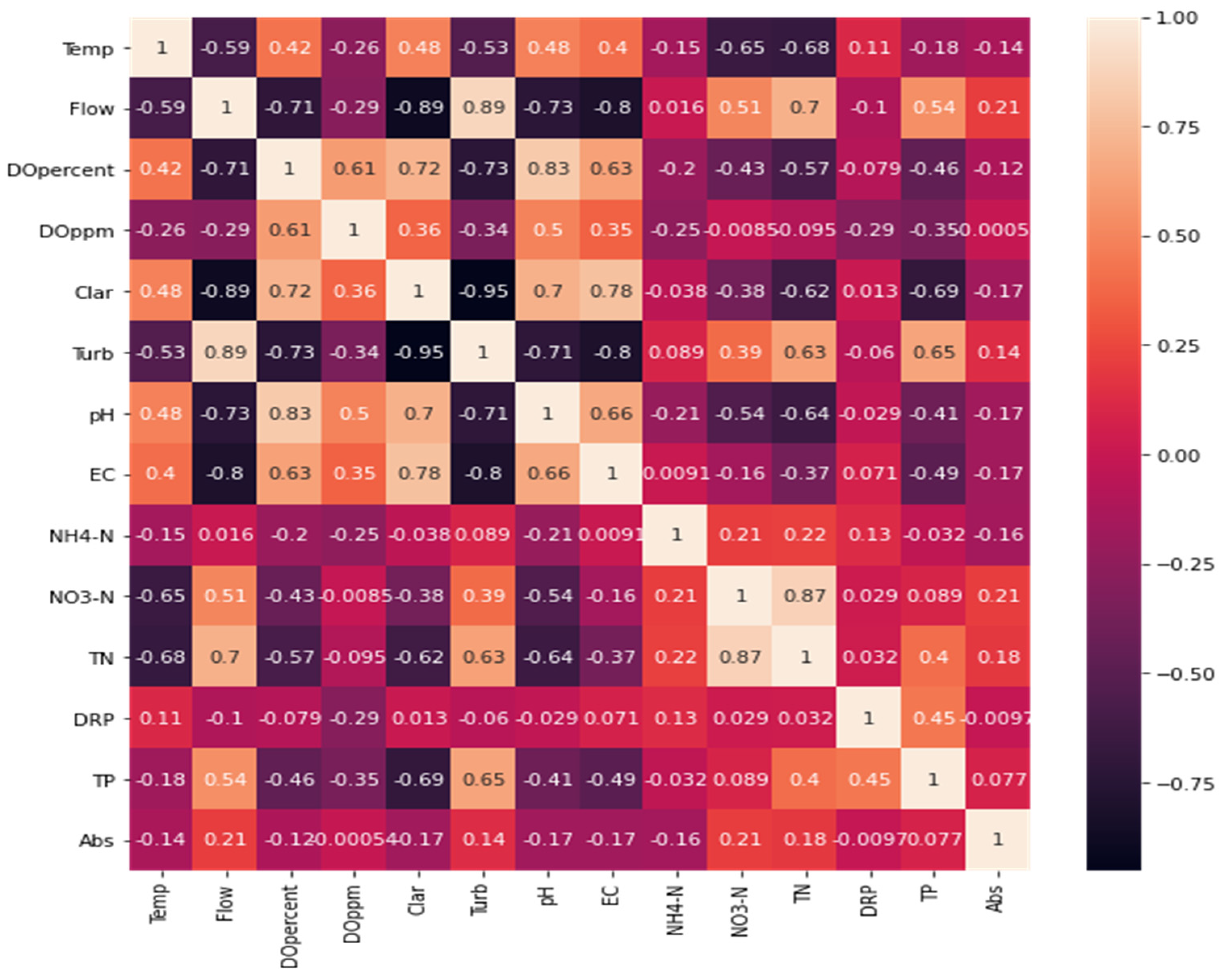
3.4. Correlation Matrix for the Different Sites

WA7, situated upstream of the Manawatu River, revealed that the flow had a strong, positive, and significant association with nutrient pollutants (NO3, TN, and TP at the 1% level) (Figure 6). Turbidity had a strong but negative correlation with other physical parameters, such as clarity and EC, at the 1% level. This relationship suggests that nutrients are introduced into the river from the surrounding land via runoff or mass weathering, and they are likely to remain undisturbed. Clarity showed an inverse relationship with TN, TP, and turbidity; however, the opposite was true for EC. These relationships suggest that a prolonged influx of pollutants into the river can obstruct river water clarity. Turbidity showed a strong positive correlation with TP and TN.
Soil matter has been reported as a receptor for pollutants on land, and it enters the stream network through sediments. Therefore, this study agrees with other findings that suggest a significantly high affinity between phosphorus and sediments. In addition, a strong positive relationship was observed between DRP and TP, as well as TN and NO3, suggesting that the pairs emanate from the same non-point sources. At the same time, with increasing temperature, DO% decreased at a rate that reflected the relationship observed between the two. For site WA8 (Figure 7), DO% showed a positive and robust correlation with pH and a negative correlation with turbidity and TP at the 1% significance level. Flow showed a consistent relationship with TP, TN, EC, turbidity, and clarity, as reported in the WA7 site. Again, clarity was inversely correlated with turbidity and TP, but proportional to EC. DO% showed strong negative relationships with turbidity and TP but was positively correlated with pH. The downstream site (WA9) showed several strong statistical relationships based on the research cut-off points. Turbidity increased with flow, whereas EC and clarity decreased under high-flow conditions (Figure 8). Similarly, the turbidity increase was associated with a decrease in clarity and EC, suggesting that the elevated EC measurements are likely to be from metallic salts instead of organic pollutants. This revealed that NH4+and TN possibly entered the river from the same source, showing strong positive statistically significant relationships at the 1% level.

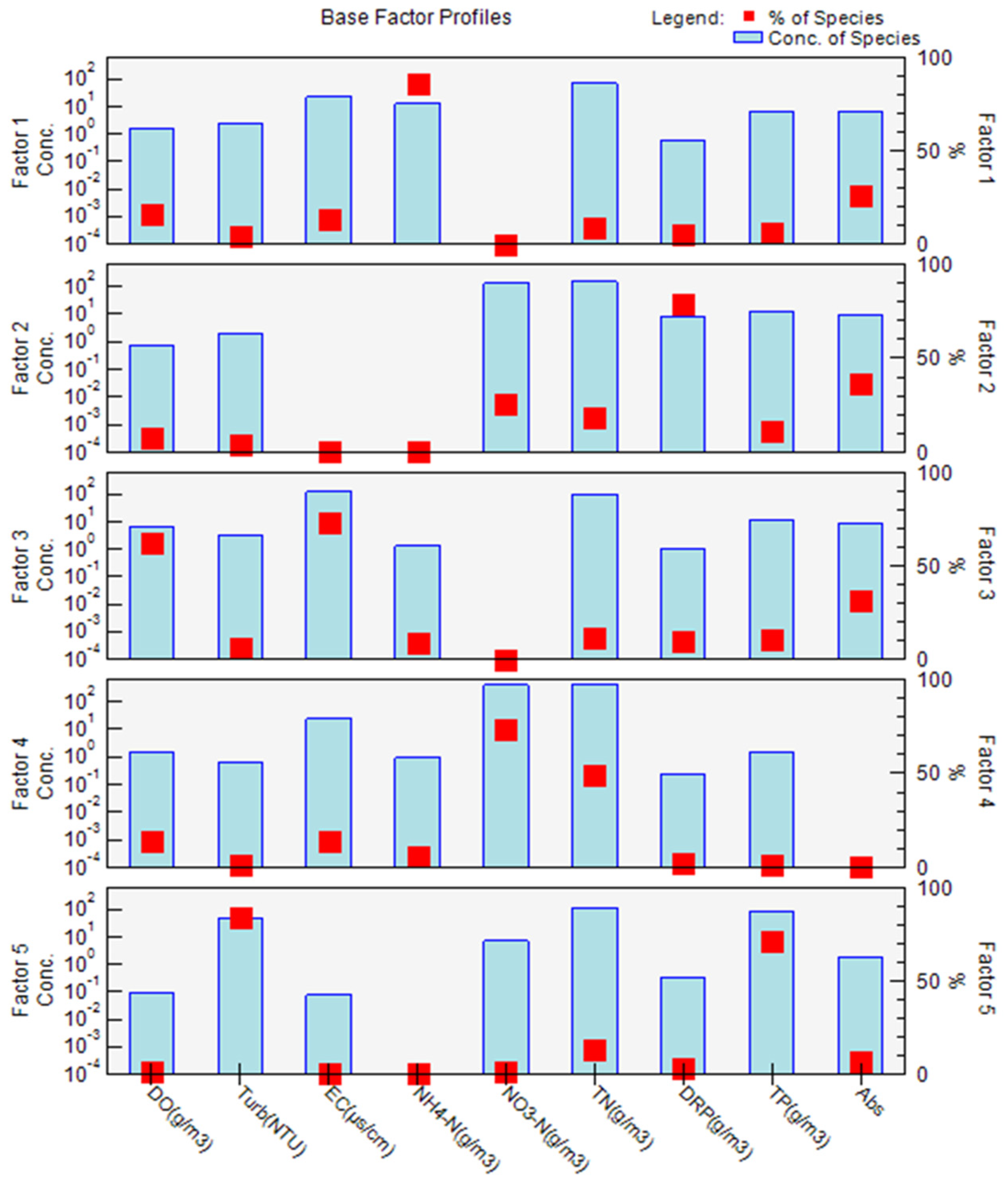
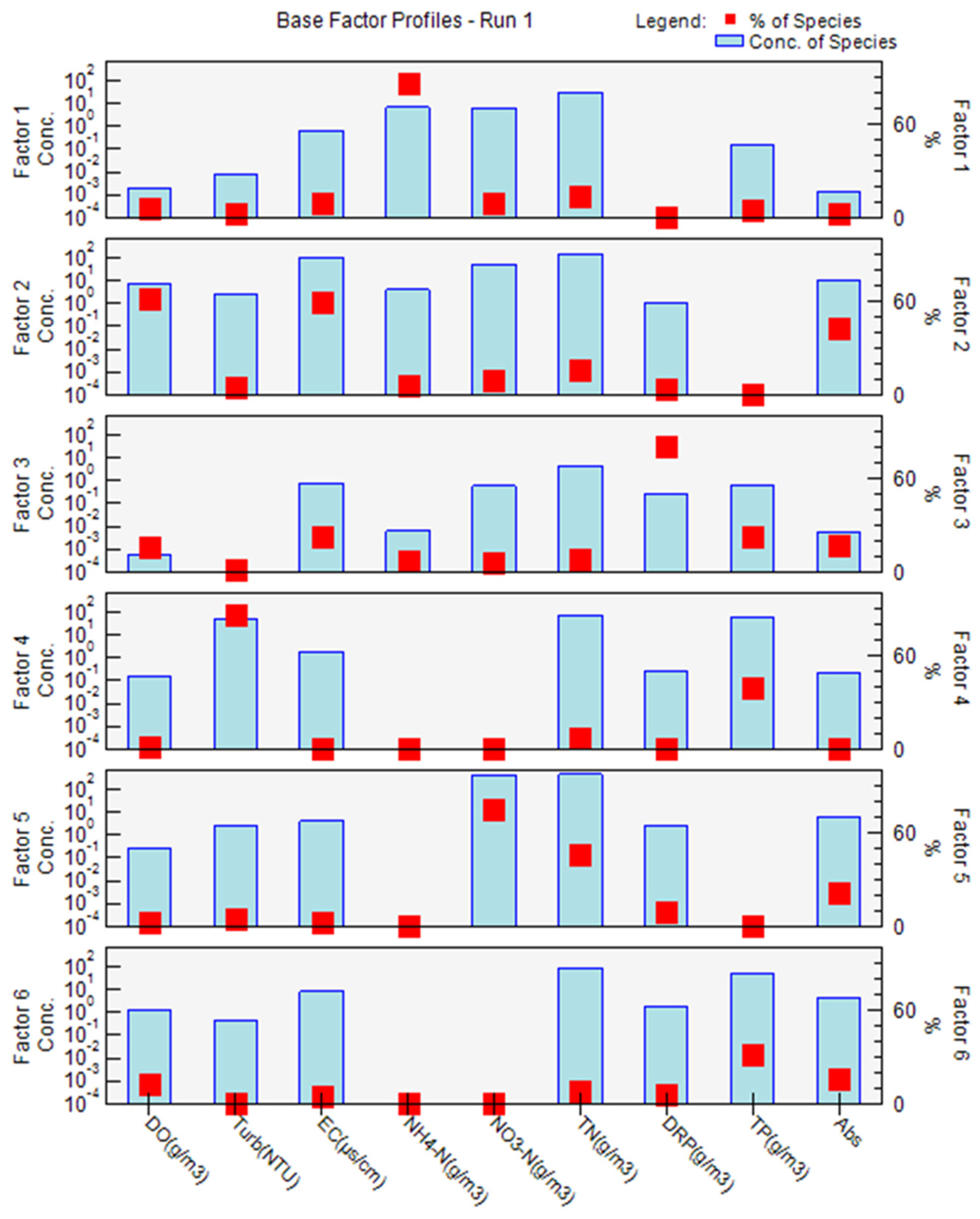
3.5. Potential Pollution Sources Using the Positive Matrix Factorization Method

The PMF method was applied to interpret potential pollution sources using the EPA-PMF 5.0 software package. The receptor modeling technique was performed in accordance with the expected output from a combination of base model displacement, base model bootstrapping, and base model BS-DISP methods [36]. These techniques were applied using trial and error, usually by selecting several factors in sequence, and ensuring that all modeling conditions were met with minimum errors occurring; the optimal R2 was set manually. Figure 9, Figure 10 and Figure 11 show the result from the extraction and modeling process, called the factor profile, and it is measured as a percentage (small red boxes). Four factors were generated for site WA7 (Figure 9), as follows: DRP (100%), NH4+ (79.1%), and CDOM (45.3%) in Factor 1; TN (59.3%) and NO3 (84%) in Factor 2; turbidity (83.9%) and TP (58.9%) in Factor 3; and DO (59.2%) and EC (73.1%) in Factor 4. For WA8 (Figure 10), Factor 1 was dominated by NH4+ (85.6%); factor 2 selected DRP (78.8%) and CDOM (36.1%); Factor 3 selected EC (72.7%) and DO (62.1%); Factor 4 selected NO3 (73.5%) and TN (48.9%); and Factor 5 selected turbidity (84.2%). Finally, six factors were extracted for WA9 (Figure 11). Factor 1 selected NH4+ (86.6%); Factor 2 selected DO (61.4%) and CDOM (42.4%); Factor 3 selected DRP (80.4%); Factor 4 selected turbidity (85.5%) and TP (39.4%); Factor 5 selected NO3 (75.4%) and TN (46.4%); and Factor 6 selected TP (32.2%).

3.6. Model Performance of PMF for Manawatu Catchment

The PMF model output showed outstanding performance in terms of modeling the trends and explaining the variability of each variable. The R2 produced showed that except for DO, NH4+, and CDOM, other variables were well predicted for WA7 in the following order: DO (0.15) < CDOM (0.45) < NH4+ (0.62) < EC (0.76) < DRP (0.84) < turbidity (0.96) < TP (0.98) < TN (0.98) < NO3 (0.99). For WA8, R2 values for each variable were as follows: DO (0.23) < aCDOM (0.54) < EC (0.84) < TP (0.94) < DRP (0.99) < NO3-N (0.99) < NH4-N (0.99) < TN (0.98) < turbidity (0.93). For the WA9 site, the R2 values were in the following order: CDOM (0.05) < DO (0.78) < EC (0.80) < TN (0.97) < TP (0.98) < turbidity (0.98) < DRP (0.99) < NO3-N (0.99) < NH4-N (0.99).

4. Discussion

4.1. Land Connectivity and Effects on Water Quality

The rivers within the Manawatu catchment have poor water quality, with median nutrient values above the ANZECC trigger values. For TP, all three stations had 5 year median values above the ANZECC threshold, with the highest TP values measured at WA9. Thus, the baseline phosphorus concentrations reveal a legacy of catchment sources that go beyond the inputs from storm events. The rainfall plots show that periods of high rainfall did not correspond with high TP values. Although high TP values were observed at the three stations in 2004, the overall rainfall pattern suggests that in-channel erosion was more likely to be the source of TP pollution. From the land-use analyses (Figure 3), it was apparent that high-producing grasslands (66%) were the dominant land-use class. However, connectivity analyses showed that a large amount of TP was introduced through the watershed from upstream (WA7).
Connectivity analyses revealed a large area of high-producing grassland connected to the floodplain. Several studies have shown that high-producing grasslands are a significant source of TP, among other nutrients [11,21,44]. The seasonality effect showed that TP values were higher than the standard in both summer and winter for all three stations, except WA9 in the summer. This also underscores that there is no direct relationship between rainfall patterns and recorded TP. The TP values may have been continuously and gradually introduced from sources other than those directly from the watershed. The gradual release of TP may have been influenced by in-channel erosion or the presence of riparian buffers. The presence of riparian buffers can limit the runoff rate and reduce the concentration of pollutants in rivers. A similar pattern was observed for DRP, NH4+, turbidity, TN, and NO3. The observed trends suggest that these pollutants were released after a storm event. In the rainfall graphs, spikes were observed in 1995, 2004, and 2011.
The storm events in 2004 and 2011 were similar in magnitude, but they did not release the same number of pollutants. This pattern may be attributed to the presence of riparian buffers, as well as scaled-back fertilizer application over time. This finding corroborates the findings in the study by Abbott et al. [31]. They found that despite landslides occurring in the Manawatu catchment, minimal suspended solids (SS) are transported into the river because only a small fraction of upland LU/LC is connected. Similar increasing trends in NH4+, NO3, and TN were observed for all three sites; however, a different pattern was observed for NH4+. The similarity between WA7 and WA8 for NO3 and TN suggests that both sites received considerable NO3 and TN pollution. However, a disproportionate amount of NH4+ was observed at different sites. Higher values of NH4+ were observed in WA9 than in the other two sites (WA7 or WA8). The reason for this is likely the presence of urban settlements that produce substantial amounts of waste rich in NH4+.

4.2. Water Quality Assessment

Analyses of 25 years of consistent river water quality data provided remarkable insights into the pollution status of the Manawatu catchment. The results for all sites clearly show that pollution varied over time and were mostly above ANZECC trigger values. High pollution (sediment and nutrients) was observed between 2000 and 2004 at all three sites. This was a response to a major storm and increased rainfall compared with other years.
These findings were revealed by post hoc tests of medians, which showed a statistical difference in nutrient concentrations. The increase in nutrients has been attributed to extreme rainfall events in the catchment between 2000 and 2004 (Figure 12). In accordance with Dymond et al. [14], rainfall was significantly elevated in February 2004. It was responsible for flushing a large amount of sediment and nutrients into the river, particularly in 2004 and 2011. Records show that the lower North Island experienced a large storm, with over 20 h of rainfall during that period. Abott et al. [31] reported that a significant storm produced an exceptional amount of sediment, especially in the loose and hilly terrain of the Manawatu watershed. The substantial increase in nutrients and sediments during the 2000–2004 period proves that a large amount of the eroded soil transporting these pollutants was deposited at that time. Consequently, these findings are corroborated with the findings in the studies of Larned et al. [27] and Kamarinas et al. [43], as they revealed that water quality in NZ is poor and will continue to degrade due to a cyclic influx of nutrients that have accumulated in the soil for up to 50 years.
Turbidity, electrical conductivity, total phosphorus, and absorbance are significant pollutants. Previous studies have shown that turbidity results from soil erosion and runoff processes [45,46,47,48]. However, it is more likely that these pollutants originated from in-channel sources. In the Manawatu River catchment, in-channel sources emanate from floodplains that trap sediments and nutrients over time and release them during rainfall. Electrical conductivity can also be a marker for the influence of mass weathering effects on water quality [49], whereas high loadings of TP stem from fertilizer application in intensive agricultural areas [46,50]. Finally, high loadings of CDOM represent the presence of dissolved organic matter comprising humic substances [51]. Cruz et al. [50] reported that TP and NO3-N entered the Siriri River in Brazil, but the sources of this pollution were different. The correlation matrix in our study showed that TP was correlated with turbidity and TN, suggesting that they emanate from the same source. As established earlier, turbidity likely originated from soil erosion. Therefore, NO3 and TN are nutrients deposited around the river’s soil.
Woldeab et al. [12] reported that TN, DRP, and NO3 were prevalent and significantly higher in vegetated and agricultural areas. NH3-N (NH4+) can be attributed to dissolved livestock manure within the watershed. Therefore, because DRP is correlated with TP, with DRP as a constituent of TP, it can serve as a possible indicator of a natural pollution source from soil erosion. Dymond et al. [14] reported that the soil material in Manawatu is rich in phosphorus. Table 3a shows that in WA7, large areas of high-producing grassland (73.5 km2) are connected to the river. This makes it highly likely that agricultural pollution enters the floodplain quickly and significantly. Similarly, Kamarinas et al. [43] revealed that high-producing grasslands and plantation forests produce substantial sediments.
A significant increase in pollution was observed in WA8, as the proportion of plantation forests and high-producing grasslands connected to WA8 increased. This finding is supported by the study by Julian et al. [21]. They reported that the amount of NOx leaking into most rivers in NZ has increased since 1989, despite the reduction in fertilizer application since the early eighties, and that it is consistent with an increase in turbidity and nutrients observed in lowland rivers [47]. The NO3 and TN at site WA9 may be due to the runoff of domestic sewage from nearby wastewater treatment plants and urban areas. One of the attributes of this site is that it has a wastewater treatment plant installed to treat waste from both industrial and domestic sources. This finding is supported by Alves et al. [52], who reported that the presence of organic matter in water could be attributed in no small amount to domestic sewage and industrial wastewater that could have been treated using traditional methods. Nutrient pollution seems likely because the downstream site had a wastewater treatment plant installed. Therefore, based on the large variability in NO3 and TN within this site, it is safe to suggest that NH4+originated from aerobic pollution caused by domestic or livestock waste. Moreover, NH4+, DRP, and TP are attributed to the effects of agricultural land use, specifically fertilizer application and animal waste [53].
Factor 2 showed high loadings of NO3, TN, and DO (Figure 9). This can be attributed to the presence of sufficient oxygen, which can play a significant role in the oxidation of nutrients entering the river from fertilizer application, causing degradation. Therefore, it is not surprising to find NH4+ in Factor 1, which could be an oxidation byproduct of NO3and TN. Factor 3 selected turbidity and TP, and this factor can be related to soil erosion. Factor 4 has been described as a physiochemical source. For WA8, high loadings of TP and turbidity may likely be attributed to soil erosion or mass weathering, as represented in Factor 1 (Figure 10). Factor 3 may be classified as agricultural pollution. Shrestha and Kazama [48] reported that nitrogen compounds were found in the Fuji River because of the application of nitrogenous fertilizers on agricultural lands around the river. Kazama and Yoneyama [54] reported similar findings. Factor 2 was likely a physiochemical source because of the presence of EC and DO. Factor 4 can be described as pollution from livestock and agricultural waste. In WA9, NH4+ was dominant, and it was likely released from domestic sewage (Figure 11). As reported in the literature, studies have shown that NH4+ can be released from several sources. These sources depend on typical land use or anthropogenic activities associated with pollution sites. However, a high percentage of NH4+ can be attributed to runoff from industrial wastewater treatment plants or domestic sewage. These findings align with the findings of Haji et al. [55], which proved that large loadings of ammoniacal-N emanated from an industrial or domestic source.
The high presence of DRP in Factor 2 in WA9 indicates the likely presence of nutrients from agricultural catchments. It is important to note that WA9 is a larger watershed encompassing WA8 and WA7. WA8 and WA7 empty into WA9, with higher agricultural practices occurring in WA7 and WA8, which could be the likely reason for the high DRP. The high presence of TP and turbidity in Factor 3 can be attributed to mass weathering pollution, one of the characteristics of lowland catchments. EC and DO in Factor 4 represent physicochemical source pollution. In contrast, factors 5 and 6 represent organic and agricultural pollution sources based on the presence of CDOM and nutrients. The results of the watershed connectivity model supported these findings. Table 3 reveals less coverage of plantation forests and high-producing grasslands within this watershed, which is a conduit for transporting pollutants into the river. Julian et al. [21] reported that high-producing grasslands increased nutrients significantly in NZ rivers, and it will likely continue to increase from legacy nutrient stores throughout the catchment.
The observations from this study are likely to be skewed in this regard, as elevated concentrations of nutrients (TN, NH4 -N, TP, and DRP) and sediment loads were recorded across New Zealand. This resulted from the presence of cattle, deer, and dairy cattle [25,28,56]. The findings of Julian et al. [21] further support these findings, as it has been reported that the number of sheep stocks in the uplands, where steep slopes are present, is higher than in the lowlands in New Zealand. As more livestock gather, intensive grazing and the movement of livestock can expose the soil to erosion. Additionally, between the early 1990s and 2012, the number of dairy cattle in NZ increased by a factor of two, which resulted in a significant increase in the application of P and N fertilizers to meet feed demands. When lactating dairy cows graze on pastures treated with P- and N-based fertilizers, approximately 0.8 and 0.6 of the total amounts of P and N fertilizer used, respectively, is deposited on the soil as animal waste [57]. In accordance with Ledgard [58], these values remain underestimated because different dairy pastures are likely to incorporate extra atmospheric N through pasture grazing, strip grazing, and cropping harvest. Pasture grazing is predominant in NZ and has been identified as the root cause of soil catchment exposure to erosion [21]. These findings support the findings from our study as more nutrients, and higher sediment loads, were characteristic of sites within the Manawatu Catchment, wherein large areas of plantation forest (PF) and high-producing grassland (HG) were connected to the floodplain.
The broader impacts of our study will be relevant for receiving waters such as lakes and bays. A study by Abell et al. [59] concerning 101 national lakes showed that high-producing grasslands increased mean TP and TN concentrations. A similar study was carried out by Özkundakci et al. [60], which revealed that high-producing grasslands also increased nutrients in 25 national lakes. The Manawatu River drains into an open estuary, and farther out to the South Taranaki Bight, neither of which is monitored as comprehensively as the river. However, we do know that there are frequent warnings following rainfall in the catchment that discourage contact recreation in the estuary due to the water quality issues we have outlined in this article.

5. Conclusions

This study aimed to identify pollutants and their potential sources within the Manawatu River catchment using multivariate statistical methods to assess the relationships between LULC, watershed connectivity, and water quality. High-producing grassland was interpreted to be the dominant pollution source at all sites. At the same time, greater urban coverage in the western part of the catchment increased pollution in the downstream section (WA9), especially for NH4+. Connectivity analyses revealed that 73.4% of the entire catchment was dominated by high-producing grassland, and 43.3% was directly connected to streams via runoff. Domestic pollution sources were mostly found in the downstream section of the Manawatu catchment. Connectivity studies also revealed the role of LULC in water quality, as high-producing grassland areas contributed to increased pollution at a higher rate than the other LULCs combined. Furthermore, this study revealed that nutrients such as TP and TN showed declining trends in concentration at all three sites; however, all median values remained above the ANZECC trigger values. NH4+ also decreased significantly in WA8, but it remained elevated in WA7 and WA9. NO3 declined to numbers below the trigger values in lowland rivers over time, and it remained of inferior quality in the upland sub-catchment.
The extremely low or insignificant rates at which pollutant concentrations decline could be a cause of concern. The introduction or improvement of retention capacities in the wetlands and riparian buffers, in location-specific areas, would be a viable solution for the Manawatu catchment area. In general, the PMF revealed that point, natural, and agricultural sources were responsible for the pollution in the downstream section of the river. In the intermediate sub-catchment, soil/bank erosion and agricultural sources were the major contributors. Agricultural pollution and soil erosion were likely responsible for the pollution in the upstream section of the catchment. Future work within the Manawatu River catchment should include the development of reaeration models to provide insight into its assimilatory capacity. Risk analyses are necessary to determine the health risks associated with using the Manawatu River in agricultural and pastoral farming. Lastly, this study showed the need for continuous and consistent water quality monitoring to evaluate water quality variables and the effectiveness of current wetlands or riparian buffers already in place. Finally, effectively tracking pollution sources, to determine which portion of a watershed should have a riparian buffer installed, remains a major challenge that water resource managers face worldwide.

Author Contributions

All authors contributed to the study conception and design. Material preparation, data collection, spatial and statistical analysis were performed by J.P.J., P.C.E., N.D.-B., O.M., S.E.S., E.O.B. and D.D.A. The first draft of the manuscript was written by I.T.T. and all authors commented on previous versions of the manuscript. All authors have read and agreed to the published version of the manuscript.

Funding

The authors declare that no funds, grants, or other support were received during the preparation of this manuscript.

Data Availability Statement

The authors have no affiliations with or involvement in any organization or entity with any financial interest or non-financial interest in the subject matter or material discussed in this manuscript. The dataset referenced in this manuscript is available at: https://hydrowebportal.niwa.co.nz/ accessed on 22 April 2021.

Conflicts of Interest

The authors declare that they have no known competing financial interests or personal relationships that could have appeared to influence the work reported in this paper.

References

  1. Jéquier, E.; Constant, F. Water as an Essential Nutrient: The Physiological Basis of Hydration. Eur. J. Clin. Nutr. 2010, 64, 115–123. [Google Scholar] [CrossRef] [Green Version]
  2. Mandal, P.; Upadhyay, R.; Hasan, A. Seasonal and Spatial Variation of Yamuna River Water Quality in Delhi, India. Environ. Monit. Assess. 2010, 170, 661–670. [Google Scholar] [CrossRef]
  3. Almeida, C.A.; Quintar, S.; González, P.; Mallea, M.A. Influence of Urbanization and Tourist Activities on the Water Quality of the Potrero de Los Funes River (San Luis–Argentina). Environ. Monit. Assess. 2007, 133, 459–465. [Google Scholar] [CrossRef]
  4. Chelsea Nagy, R.; Graeme Lockaby, B.; Kalin, L.; Anderson, C. Effects of Urbanization on Stream Hydrology and Water Quality: The Florida Gulf Coast. Hydrol. Process. 2012, 26, 2019–2030. [Google Scholar] [CrossRef]
  5. Peters, N.E. Effects of Urbanization on Stream Water Quality in the City of Atlanta, Georgia, USA. Hydrol. Process. 2009, 23, 2860–2878. [Google Scholar] [CrossRef]
  6. Tenebe, I.T.; Emenike, C.P.; Daniel Chukwuka, C. Prevalence of Heavy Metals and Computation of Its Associated Risk in Surface Water Consumed in Ado-Odo Ota, South-West Nigeria. Hum. Ecol. Risk Assess. Int. J. 2019, 25, 882–904. [Google Scholar] [CrossRef]
  7. ul Hassan, Z.; Shah, J.A.; Kanth, T.A.; Pandit, A.K. Influence of Land Use/Land Cover on the Water Chemistry of Wular Lake in Kashmir Himalaya (India). Ecol. Process. 2015, 4, 9. [Google Scholar] [CrossRef] [Green Version]
  8. Huang, J.; Zhan, J.; Yan, H.; Wu, F.; Deng, X. Evaluation of the Impacts of Land Use on Water Quality: A Case Study in The Chaohu Lake Basin. Sci. World J. 2013, 2013, e329187. [Google Scholar] [CrossRef] [Green Version]
  9. Tenebe, I.T.; Ogbiye, A.S.; Omole, D.O.; Emenike, P.C. Estimation of Longitudinal Dispersion Co-Efficient: A Review. Cogent Eng. 2016, 3, 1216244. [Google Scholar] [CrossRef]
  10. Tenebe, I.T.; Ogbiye, A.S.; Omole, D.O.; Emenike, P.C. Parametric Evaluation of the Euler-Lagrangian Approach for Tracer Studies. Desalin. Water Treat. 2018, 109, 344–349. [Google Scholar] [CrossRef]
  11. Larned, S.T.; Moores, J.; Gadd, J.; Baillie, B.; Schallenberg, M. Evidence for the Effects of Land Use on Freshwater Ecosystems in New Zealand. N. Z. J. Mar. Freshw. Res. 2020, 54, 551–591. [Google Scholar] [CrossRef]
  12. Woldeab, B.; Ambelu, A.; Mereta, S.T.; Beyene, A. Effect of Watershed Land Use on Tributaries’ Water Quality in the East African Highland. Environ. Monit. Assess. 2018, 191, 36. [Google Scholar] [CrossRef] [PubMed]
  13. Julian, J.P.; Gardner, R.H. Land Cover Effects on Runoff Patterns in Eastern Piedmont (USA) Watersheds. Hydrol. Process. 2014, 28, 1525–1538. [Google Scholar] [CrossRef]
  14. Dymond, J.R.; Serezat, D.; Ausseil, A.-G.E.; Muirhead, R.W. Mapping of Escherichia Coli Sources Connected to Waterways in the Ruamahanga Catchment, New Zealand. Environ. Sci. Technol. 2016, 50, 1897–1905. [Google Scholar] [CrossRef]
  15. Taiwo, A.M. Source Identification and Apportionment of Pollution Sources to Groundwater Quality in Major Cities in Southwest, Nigeria/Identifikacija Izvora Oneciscenja Podzemnih Voda u Vecim Gradovima Jugozapadne Nigerije. Geofizika 2012, 29, 157–175. [Google Scholar]
  16. Emenike, C.P.; Tenebe, I.T.; Omole, D.O.; Ngene, B.U.; Oniemayin, B.I.; Maxwell, O.; Onoka, B.I. Accessing Safe Drinking Water in Sub-Saharan Africa: Issues and Challenges in South–West Nigeria. Sustain. Cities Soc. 2017, 30, 263–272. [Google Scholar] [CrossRef]
  17. Emenike, C.P.; Tenebe, I.T.; Jarvis, P. Fluoride Contamination in Groundwater Sources in Southwestern Nigeria: Assessment Using Multivariate Statistical Approach and Human Health Risk. Ecotoxicol. Environ. Saf. 2018, 156, 391–402. [Google Scholar] [CrossRef] [Green Version]
  18. Gulgundi, M.S.; Shetty, A. Identification and Apportionment of Pollution Sources to Groundwater Quality. Environ. Process. 2016, 3, 451–461. [Google Scholar] [CrossRef]
  19. Chounlamany, V.; Tanchuling, M.A.; Inoue, T. Spatial and Temporal Variation of Water Quality of a Segment of Marikina River Using Multivariate Statistical Methods. Water Sci. Technol. 2017, 76, 1510–1522. [Google Scholar] [CrossRef]
  20. Bruesewitz, D.A.; Hamilton, D.P.; Schipper, L.A. Denitrification Potential in Lake Sediment Increases Across a Gradient of Catchment Agriculture. Ecosystems 2011, 14, 341–352. [Google Scholar] [CrossRef]
  21. Julian, J.P.; de Beurs, K.M.; Owsley, B.; Davies-Colley, R.J.; Ausseil, A.-G.E. River Water Quality Changes in New Zealand over 26 Years: Response to Land Use Intensity. Hydrol. Earth Syst. Sci. 2017, 21, 1149–1171. [Google Scholar] [CrossRef] [Green Version]
  22. Schallenberg, M. Determining Reference Conditions for New Zealand Lakes. Sci. Conserv. 2019, 334, 1. [Google Scholar]
  23. OECD/FAO. Aglink-Cosimo Model Documentation—A Partial Equilibrium Model of World Agricultural Markets; FAO: Rome, Italy, 2022; ISBN 978-92-5-136969-2. [Google Scholar]
  24. Smith, D.G.; McBride, G.B. New Zealand’s National Water Quality Monitoring Network—Design and First Year’s Operation1. JAWRA J. Am. Water Resour. Assoc. 1990, 26, 767–775. [Google Scholar] [CrossRef]
  25. Davies-Colley, R.J.; Nagels, J.W.; Smith, R.A.; Young, R.G.; Phillips, C.J. Water Quality Impact of a Dairy Cow Herd Crossing a Stream. N. Z. J. Mar. Freshw. Res. 2004, 38, 569–576. [Google Scholar] [CrossRef] [Green Version]
  26. Ballantine, D.J.; Davies-Colley, R.J. Water Quality Trends in New Zealand Rivers: 1989-2009. Environ. Monit. Assess. 2014, 186, 1939–1950. [Google Scholar] [CrossRef]
  27. Larned, S.; Snelder, T.; Unwin, M.; McBride, G. Water Quality in New Zealand Rivers: Current State and Trends. N. Z. J. Mar. Freshw. Res. 2016, 50, 389–417. [Google Scholar] [CrossRef]
  28. Mcdowell, R.W.; Larned, S.T.; Houlbrooke, D.J. Nitrogen and Phosphorus in New Zealand Streams and Rivers: Control and Impact of Eutrophication and the Influence of Land Management. N. Z. J. Mar. Freshw. Res. 2009, 43, 985–995. [Google Scholar] [CrossRef]
  29. Reff, A.; Eberly, S.I.; Bhave, P.V. Receptor Modeling of Ambient Particulate Matter Data Using Positive Matrix Factorization: Review of Existing Methods. J. Air Waste Manag. Assoc. 2007, 57, 146–154. [Google Scholar] [CrossRef] [Green Version]
  30. Smith, D.G.; McBride, G.B.; Bryers, G.G.; Wisse, J.; Mink, D.F.J. Trends in New Zealand’s National River Water Quality Network. N. Z. J. Mar. Freshw. Res. 1996, 30, 485–500. [Google Scholar] [CrossRef]
  31. Abbott, S.; Julian, J.P.; Kamarinas, I.; Meitzen, K.M.; Fuller, I.C.; McColl, S.T.; Dymond, J.R. State-Shifting at the Edge of Resilience: River Suspended Sediment Responses to Land Use Change and Extreme Storms. Geomorphology 2018, 305, 49–60. [Google Scholar] [CrossRef]
  32. Hicks, D.M.; Shankar, U.; McKerchar, A.I.; Basher, L.; Lynn, I.; Page, M.; Jessen, M. Suspended Sediment Yields from New Zealand Rivers. J. Hydrol. 2011, 50, 81–142. [Google Scholar]
  33. Land Air Water Aotearoa. Available online: https://www.lawa.org.nz/download-data/ (accessed on 14 June 2023).
  34. Davies-Colley, R.J.; Smith, D.G.; Ward, R.C.; Bryers, G.G.; McBride, G.B.; Quinn, J.M.; Scarsbrook, M.R. Twenty Years of New Zealand’s National Rivers Water Quality Network: Benefits of Careful Design and Consistent Operation1. JAWRA J. Am. Water Resour. Assoc. 2011, 47, 750–771. [Google Scholar] [CrossRef]
  35. ANZECC & ARMCANZ (2000) Guidelines. Available online: https://www.waterquality.gov.au/anz-guidelines/resources/previous-guidelines/anzecc-armcanz-2000 (accessed on 8 June 2023).
  36. US EPA. Positive Matrix Factorization 5.0 Fundamentals and User Guide. Available online: https://www.epa.gov/air-research/epa-positive-matrix-factorization-50-fundamentals-and-user-guide (accessed on 14 June 2023).
  37. Kaiser, H.F. An Index of Factorial Simplicity. Psychometrika 1974, 39, 31–36. [Google Scholar] [CrossRef]
  38. Aitchison, J. Measures of Location of Compositional Data Sets. Math. Geol. 1989, 21, 787–790. [Google Scholar] [CrossRef]
  39. Blake, S.; Henry, T.; Murray, J.; Flood, R.; Muller, M.R.; Jones, A.G.; Rath, V. Compositional Multivariate Statistical Analysis of Thermal Groundwater Provenance: A Hydrogeochemical Case Study from Ireland. Appl. Geochem. 2016, 75, 171–188. [Google Scholar] [CrossRef] [Green Version]
  40. Emenike, P.C.; Tenebe, I.; Ogarekpe, N.; Omole, D.; Nnaji, C. Probabilistic Risk Assessment and Spatial Distribution of Potentially Toxic Elements in Groundwater Sources in Southwestern Nigeria. Sci. Rep. 2019, 9, 15920. [Google Scholar] [CrossRef] [Green Version]
  41. Manousakas, M.; Papaefthymiou, H.; Diapouli, E.; Migliori, A.; Karydas, A.G.; Bogdanovic-Radovic, I.; Eleftheriadis, K. Assessment of PM2.5 Sources and Their Corresponding Level of Uncertainty in a Coastal Urban Area Using EPA PMF 5.0 Enhanced Diagnostics. Sci. Total. Environ. 2017, 574, 155–164. [Google Scholar] [CrossRef] [PubMed] [Green Version]
  42. Kamarinas, I. Geospatial Analyses of Terrestrial-Aquatic Connections Across New Zealand and Their Influence on River Water Quality. Ph.D. Thesis, Texas State University, San Marcos, TX, USA, August 2018. [Google Scholar]
  43. Kamarinas, I.; Julian, J.P.; Hughes, A.O.; Owsley, B.C.; De Beurs, K.M. Nonlinear Changes in Land Cover and Sediment Runoff in a New Zealand Catchment Dominated by Plantation Forestry and Livestock Grazing. Water 2016, 8, 436. [Google Scholar] [CrossRef] [Green Version]
  44. Snelder, T.H.; McDowell, R.W.; Fraser, C.E. Estimation of Catchment Nutrient Loads in New Zealand Using Monthly Water Quality Monitoring Data. JAWRA J. Am. Water Resour. Assoc. 2017, 53, 158–178. [Google Scholar] [CrossRef]
  45. Kemker, C. Turbidity, Total Suspended Solids & Water Clarity. Available online: https://www.fondriest.com/environmental-measurements/parameters/water-quality/turbidity-total-suspended-solids-water-clarity/ (accessed on 14 June 2023).
  46. Salim, I.; Sajjad, R.U.; Paule-Mercado, M.C.; Memon, S.A.; Lee, B.-Y.; Sukhbaatar, C.; Lee, C.-H. Comparison of Two Receptor Models PCA-MLR and PMF for Source Identification and Apportionment of Pollution Carried by Runoff from Catchment and Sub-Watershed Areas with Mixed Land Cover in South Korea. Sci. Total Environ. 2019, 663, 764–775. [Google Scholar] [CrossRef]
  47. Memon, S.; Paule, M.C.; Lee, B.-Y.; Umer, R.; Sukhbaatar, C.; Lee, C.-H. Investigation of Turbidity and Suspended Solids Behavior in Storm Water Run-off from Different Land-Use Sites in South Korea. Desalin. Water Treat. 2015, 53, 3088–3095. [Google Scholar] [CrossRef]
  48. Shrestha, S.; Kazama, F. Assessment of Surface Water Quality Using Multivariate Statistical Techniques: A Case Study of the Fuji River Basin, Japan. Environ. Model. Softw. 2007, 22, 464–475. [Google Scholar] [CrossRef]
  49. Ogwueleka, T.C. Use of Multivariate Statistical Techniques for the Evaluation of Temporal and Spatial Variations in Water Quality of the Kaduna River, Nigeria. Environ. Monit. Assess. 2015, 187, 137. [Google Scholar] [CrossRef] [PubMed]
  50. Cruz, M.A.S.; Gonçalves, A.d.A.; de Aragão, R.; de Amorim, J.R.A.; da Mota, P.V.M.; Srinivasan, V.S.; Garcia, C.A.B.; de Figueiredo, E.E. Spatial and Seasonal Variability of the Water Quality Characteristics of a River in Northeast Brazil. Environ. Earth Sci. 2019, 78, 68. [Google Scholar] [CrossRef]
  51. Reynolds, D.M. The Differentiation of Biodegradable and Non-Biodegradable Dissolved Organic Matter in Wastewaters Using Fluorescence Spectroscopy. J. Chem. Technol. Biotechnol. 2002, 77, 965–972. [Google Scholar] [CrossRef]
  52. Alves, D.D.; Riegel, R.P.; de Quevedo, D.M.; Osório, D.M.M.; da Costa, G.M.; do Nascimento, C.A.; Telöken, F. Seasonal Assessment and Apportionment of Surface Water Pollution Using Multivariate Statistical Methods: Sinos River, Southern Brazil. Environ. Monit. Assess. 2018, 190, 384. [Google Scholar] [CrossRef]
  53. Dils, R.M.; Heathwaite, A.L. The Controversial Role of Tile Drainage in Phosphorus Export from Agricultural Land. Water Sci. Technol. 1999, 39, 55–61. [Google Scholar] [CrossRef]
  54. Kazama, F.; Yoneyama, M. Nitrogen Generation in the Yamanashi Prefecture and Its Effects on the Groundwater Pollution. Environ. Sci. 2002, 15, 293–298. [Google Scholar] [CrossRef]
  55. Haji Gholizadeh, M.; Melesse, A.M.; Reddi, L. Water Quality Assessment and Apportionment of Pollution Sources Using APCS-MLR and PMF Receptor Modeling Techniques in Three Major Rivers of South Florida. Sci. Total Environ. 2016, 566–567, 1552–1567. [Google Scholar] [CrossRef]
  56. Buck, O.; Niyogi, D.K.; Townsend, C.R. Scale-Dependence of Land Use Effects on Water Quality of Streams in Agricultural Catchments. Environ. Pollut. 2004, 130, 287–299. [Google Scholar] [CrossRef]
  57. Monaghan, R.M.; Hedley, M.J.; Di, H.J.; McDowell, R.W.; Cameron, K.C.; Ledgard, S.F. Nutrient Management in New Zealand Pastures—Recent Developments and Future Issues. N. Z. J. Agric. Res. 2007, 50, 181–201. [Google Scholar] [CrossRef] [Green Version]
  58. Ledgard, S.F. Nitrogen Cycling in Low Input Legume-Based Agriculture, with Emphasis on Legume/Grass Pastures. Plant Soil 2001, 228, 43–59. [Google Scholar] [CrossRef]
  59. Abell, J.M.; Özkundakci, D.; Hamilton, D.P. Nitrogen and Phosphorus Limitation of Phytoplankton Growth in New Zealand Lakes: Implications for Eutrophication Control. Ecosystems 2010, 13, 966–977. [Google Scholar] [CrossRef] [Green Version]
  60. Özkundakci, D.; Hamilton, D.P.; Kelly, D.; Schallenberg, M.; de Winton, M.; Verburg, P.; Trolle, D. Ecological Integrity of Deep Lakes in New Zealand across Anthropogenic Pressure Gradients. Ecol. Indic. 2014, 37, 45–57. [Google Scholar] [CrossRef]
Figure 1. Manawatu River catchment showing major river networks and sampling sites.
Water 15 02939 g001
Figure 2. Landscape connectivity map for the Manawatu River Catchment.
Water 15 02939 g002
Figure 3. Land Use Land Cover (LULC) map for Manawatu River Catchment.
Water 15 02939 g003
Figure 4. (aj): Water Quality patterns for 25 years, at 5-year intervals, at the three stations. The red lines represent the ANZECC trigger values for the respective WQ variables.
Water 15 02939 g004
Figure 5. (aj): Water Quality patterns for 25 years, at the three stations, in different seasons. The red lines represent the ANZECC trigger values for the respective WQ variables.
Water 15 02939 g005
Figure 6. Spearman’s correlation matrix for Site WA7.
Water 15 02939 g006
Figure 7. Spearman’s correlation matrix for Site WA8.
Water 15 02939 g007
Figure 8. Spearman’s correlation matrix for Site WA9.
Water 15 02939 g008
Figure 9. Profile concentrations for WA7 using PMF.
Water 15 02939 g009
Figure 10. Profile concentrations for WA8 using PMF.
Water 15 02939 g010
Figure 11. Profile concentrations for WA9 using PMF.
Water 15 02939 g011
Figure 12. Mean annual rainfall for Palmerston North in the Manawatu Catchment.
Water 15 02939 g012
Table 1. Characteristics and location of monitoring sites in the Manawatu Catchment.
Site CodeCatchment Area (km2)Site Description
WA7705.28Located upstream
WA83897.37Major river mid-stream located in the center of Palmerston North
WA94222.22Located downstream
Table 2. Description of Water Quality Data Used for Analysis of the Manawatu River in NZ from 1989–2014.
UnitAbbreviationMissing Data (%)Trigger Values (Lowland/Upland )
Flow ratem3/sFlow1.4
Water Temperature°CTw0.3
Electrical conductivityµScm−1EC-
Dissolved Oxygeng/m3DO1.36
Dissolved Oxygen (%)%DO%1.398/99
pH-pH0.27.2/7.3
TurbidityNTUTurb-5.6/4.1
Total Phosphorusg/m3TP0.333/26
Total Nitrogeng/m3TN0.6614/295
Visual claritym−1Clar-0.8/0.6
Dissolved Reactive Phosphorusg/m3DRP-10/9
Ammoniacal nitrogeng/m3NH4-N-21/10
Nitrateg/m3NO3-N-444/167
Note: DO % and pH: lower limits were considered. Lowland and Upland are distinguished by the 150-m elevation threshold.
Table 3. (a) Reclassified watershed properties for WA7. (b) Reclassified Watershed Properties for Site WA8. (c) Reclassified Watershed Properties for Site WA9.
Land Use/
Land Cover Category
Connected Area in Floodplain (km2)Connected Area Not in Floodplain (km2)Area Not Connected (km2)Total (km2)
(a)
Shrub/grassland3.3914.2015.6733.26
Urban0.120.120.360.60
Non-plantation forest2.6910.9210.9924.60
Plantation forest3.366.7711.1121.24
Vegetated wetland0.000.010.030.04
High-producing grassland73.47163.76386.83624.06
Open water0.490.280.491.26
Barren/other0.050.080.090.22
Perennial cropland----
Annual cropland----
Total (km2)83.57196.14425.57705.28
(b)
Shrub/grassland47.51294.89207.40549.80
Urban1.932.4517.5321.91
Non-plantation forest35.27174.98100.38310.63
Plantation forest11.7828.2750.5590.60
Vegetated wetland0.10.180.580.86
High-producing grassland332.21756.141799.322887.67
Open water6.863.344.2614.28
Barren/other3.753.773.1910.71
Perennial cropland0.070.070.310.45
Annual cropland1.431.197.6610.28
Total (km2)440.911265.282191.183897.37
(c)
Shrub/grassland52.08319.23225.73597.04
Urban5.305.7339.2950.32
Non-plantation forest37.51181.05105.76324.32
Plantation forest14.0935.2760.82110.18
Vegetated wetland0.100.180.580.86
High-producing grassland360.67792.611944.123097.40
Open water8.013.825.0516.88
Barren/other4.223.923.4511.59
Perennial cropland0.080.090.410.58
Annual cropland1.851.7010.0813.63
Total (km2)483.911343.602395.294222.22
Disclaimer/Publisher’s Note: The statements, opinions and data contained in all publications are solely those of the individual author(s) and contributor(s) and not of MDPI and/or the editor(s). MDPI and/or the editor(s) disclaim responsibility for any injury to people or property resulting from any ideas, methods, instructions or products referred to in the content.

