Article

An Integrated GIS and Machine-Learning Technique for Groundwater Quality Assessment and Prediction in Southern Saudi Arabia

1
Civil Engineering Department, Faculty of Engineering, Minia University, Minia 61111, Egypt
2
Civil Engineering Department, College of Engineering, Shaqra University, Dawadmi 11911, Saudi Arabia
3
National Centre for Groundwater Research and Training, College of Science and Engineering, Flinders University, GPO Box 2100, Adelaide, SA 5001, Australia
4
Abdullah Alrushaid Chair for Earth Science Remote Sensing Research, Geology and Geophysics Department, College of Science, King Saud University, Riyadh 11451, Saudi Arabia
5
Agricultural Engineering Department, Faculty of Agriculture, Mansoura University, Mansoura 35516, Egypt
*
Authors to whom correspondence should be addressed.
Water 2023, 15(13), 2448; https://doi.org/10.3390/w15132448
Submission received: 27 April 2023 / Revised: 22 June 2023 / Accepted: 27 June 2023 / Published: 4 July 2023
(This article belongs to the Special Issue Water Quality, Water Security and Risk Assessment)

Abstract

:
One of the most critical stages for developing groundwater resources for drinking water use is assessing the water quality. The use of a Water Quality Index (WQI) is considered an effective method of evaluating water quality. The objective of this research was to evaluate the performance of six multiple artificial intelligence techniques, i.e., linear regression (stepwise), support vector regression SVM (linear and polynomial kernels), Gaussian process regression (GPR), Fit binary tree, and artificial neural network ANN (Bayesian) to predict the WQI in Jizan, Southern Saudi Arabia. A total of 145 groundwater samples were collected from shallow dug wells and boreholes tapping the phreatic aquifer. The WQI was calculated from 11 physicochemical parameters (pH, TDS, Ca2+, Mg2+, Na+, K+, Cl, SO42−, HCO3, NO3, and TH). The spatial distribution results showed that higher values of Cl and SO42− were recorded in the places close to the coastline, indicating the occurrence of seawater intrusion and salinisation. Seven wells had a WQI of greater than 300, indicating that the water was unfit for consumption. The results showed that the GPR, linear regression (stepwise), and ANN models performed best during the training and testing stages, with a high correlation of 1.00 and low errors. The stepwise fitting model indicated that pH, K+, and NO3 were the most significant variables, while HCO3 was a non-significant variable for the WQI. The GPR, stepwise regression, and ANN models performed best during the training and testing stages, with a high correlation and low errors. In contrast, the SVM and Fit binary tree models performed the worst in the training and testing phases. Based on subset regression analysis, the optimum input combination for WQI model prediction was determined as these eight input combinations with high R2 (0.975–1.00) and high Adj-R2 (0.974–1.00). The resultant WQI model significantly contributes to sustainable groundwater resource management in arid areas and generates improved prediction precision with fewer input parameters.

1. Introduction

Groundwater plays an essential role in the overall use and management of water resources. The demand for groundwater for municipal, agricultural, and industrial use has grown gradually during the past decades, especially in arid regions like Saudi Arabia, where groundwater is the primary source of water. In Saudi Arabia, groundwater contributes to nearly 79% of the total water supply, and around 90% is consumed in agricultural activity. Many cities, towns, and villages rely exclusively on wells and natural springs for their municipal water [1,2].
Groundwater quality is determined by the natural and physical state of the water-rock interactions and by the changes induced by human activities [3]. Groundwater contamination is generally due to urbanisation, industrialisation, and agriculture that has gradually developed over the years without considering environmental consequences [4]. Water quality assessments aim to characterise the chemical, physical, and biological conditions of groundwater and identify the source of any possible contamination that causes water quality degradation [5]. Generally, groundwater quality parameters are compared with permissible levels for a particular use to help indicate contamination sources [6,7,8]. The assessment of groundwater quality depends mainly on laboratory investigations carried out through the measurement of water quality variables, followed by a comparison of the obtained concentrations with the standards and guidelines [9]. Applied methodologies for water quality assessment often combine all the variables and present a final value as a quality index providing meaningful summaries of water quality data useful to technical and policy individuals and the public interested in water quality [10].
Geographical information systems (GIS) can be a great complementary tool for creating and developing spatial representations of water quality assessments [8,11]. Gunduz and Simsek [12] and Usali and Ismail [13] applied a GIS-integrated technique to assess irrigation water quality in respectively, Turkey and Malaysia. They concluded that water quality parameters could be produced in the form of a map using model-based GIS techniques and considered this product as the most suitable method for groundwater potential prediction zoning.
The application of a Water Quality Index (WQI) is considered an effective method for evaluating water quality [14]. A WQI is a premium method for understanding and summarising large numbers of water quality data by integrating complex information and expressions to represent a combined effect of the variables influencing water quality. Thus, a WQI enables effective monitoring and evaluation of groundwater quality. Over the last few decades, WQIs have been widely used for surface water and groundwater quality assessments worldwide [15,16]. There are many water quality indices, such as the Weighted Arithmetic Water Quality Index (WAWQI), National Sanitation Foundation Water Quality Index (NSFWQI), Canadian Council of Ministers of the Environment Water Quality Index (CCMEWQI), and Oregon Water Quality Index (OWQI). National and international organisations have formulated these indices dependent on a number of water quality parameters relative to the specific requirements of a given area [17,18]. Water quality indices have been shown to demonstrate temporal and spatial differences in water quality, even at small concentrations, in an accurate and timely manner [19].
There is a current rise in the use of artificial intelligence (AI) techniques to estimate WQIs [20,21,22,23,24]. Groundwater quality can be understood and monitored using artificial neural networks (ANNs) and used to predict water quality with great success [25,26,27]. Also, other computational intelligence techniques, such as genetic algorithms (GA), support vector machine (SVM), Fit binary Tree, and Gaussian process regression (GPR), have attracted growing interest in WQI prediction studies [28,29]. The non-linear structure of computational intelligence techniques and their ability to anticipate complex occurrences, handle massive datasets of varying sizes, and accommodate missing data are all advantages. Additionally, artificial intelligence approaches have been shown to be extremely capable of forecasting water quality [26,27,30,31,32,33,34,35,36].
Gazzaz et al. [30] applied a neural network model for calculating a WQI for the Kinta River, Malaysia. The model’s WQI predictions were highly correlated with measured WQI values (r = 0.977). El Bilali and Taleb [31] used eight machine learning (ML) models: artificial neural network (ANN), multiple linear regression (MLR), decision tree, Random Forest (RF), support vector machine (SVM), k-nearest neighbour (kNN), stochastic gradient descent (SGD), and adaptive boosting (AdaBoost) to forecast ten irrigation water quality (IWQ) parameters in the Bouregreg watershed, Morocco. The findings of the machine learning models showed that they are cost-effective tools for predicting irrigation water quality. Kulisz et al. [33] developed an ANN model using five parameters (EC, pH, Ca, Mg, and K) to forecast a groundwater WQI in Syczyn, Poland. It was concluded that the ANN tools predicted the WQI at a desirable level of accuracy (r = 0.9992). Kouadri et al. (2021) used eight artificial intelligence algorithms: MLR, RF, M5P model tree, random subspace (RSS), additive regression (AR), ANN, SVR, and locally weighted linear regression (LWLR) to predict a WQI in Illizi region, southeast Algeria. The MLR model had a higher level of accuracy when compared to other models. Gupta et al. [32] employed machine learning algorithms to evaluate a WQI in India’s Mid Gangetic Region. They concluded that machine learning models are a suitable alternative for groundwater water quality evaluation and may be applied swiftly utilising a data-driven approach. Setshedi et al. [26] employed an ANN to build the best model for forecasting water quality metrics using data from three district municipalities in the Eastern Cape Province, South Africa. The findings revealed that the ANN model is a valuable and reliable tool for optimising the observational network by identifying key monitoring sites and accurately forecasting the quality of river water variables. Mokhtar et al. [27] applied three artificial intelligence (AI) and four multiple regression models to forecast six irrigation water quality criteria. The findings indicated that these models could be used to make quick decisions about irrigation water quality.
To the best of our knowledge, no research has been published that evaluates the performance of artificial intelligence approaches to predict WQIs in the area of Jazan and Tihama plains in the southwestern part of the Red Sea coast of Saudi Arabia. The choice of the study area takes into consideration its importance to national development in the Kingdom. The study area and its surroundings are considered one of the most promising areas in agricultural and industrial development. Thus, the evaluation of the Water Quality Index in the study area could be useful to help planners and decision-makers to protect groundwater resources from deterioration.
Hence, the goal of this research is to (i) test a number of advanced artificial intelligence techniques in their capacity to estimate a WQI using 11 physicochemical parameters (pH, TDS, Ca2+, Mg2+, Na+, K+, Cl, SO42−, HCO3, NO3, and TH) collected from 145 groundwater wells in Jizan, Saudi Arabia, and (ii) to select the statistically optimal artificial intelligence model in predicting a WQI. The following steps were taken to achieve this goal. Firstly, the statistical analysis and correlation coefficients for the physicochemical parameters were determined. Secondly, ArcGIS was used to create maps of the spatial distribution of groundwater quality metrics. Thirdly, the Weighted Arithmetic Water Quality Index (proposed by Horton [37]) was used to calculate the WQI. Fourthly, to predict the WQI, multiple artificial intelligence techniques were used (linear regression (stepwise), SVM (linear and polynomial kernels), Gaussian process regression (GPR), Fit binary tree, and ANN (Bayesian)). Finally, the best subset regression analysis was performed to determine the best input combinations for the WQI model. This study presents two essential findings, which are as follows: (1) Creating a single-line linear equation that can be easily applied by water users and decision makers when all parameters are available (11 inputs); (2) when data are limited, we used the best subset regression model to extract the optimal input parameters to the ML model for WQ prediction. As a result of this research, two future plans/strategies for water quality simulations will be developed.

2. Materials and Methods

2.1. Study Area Description

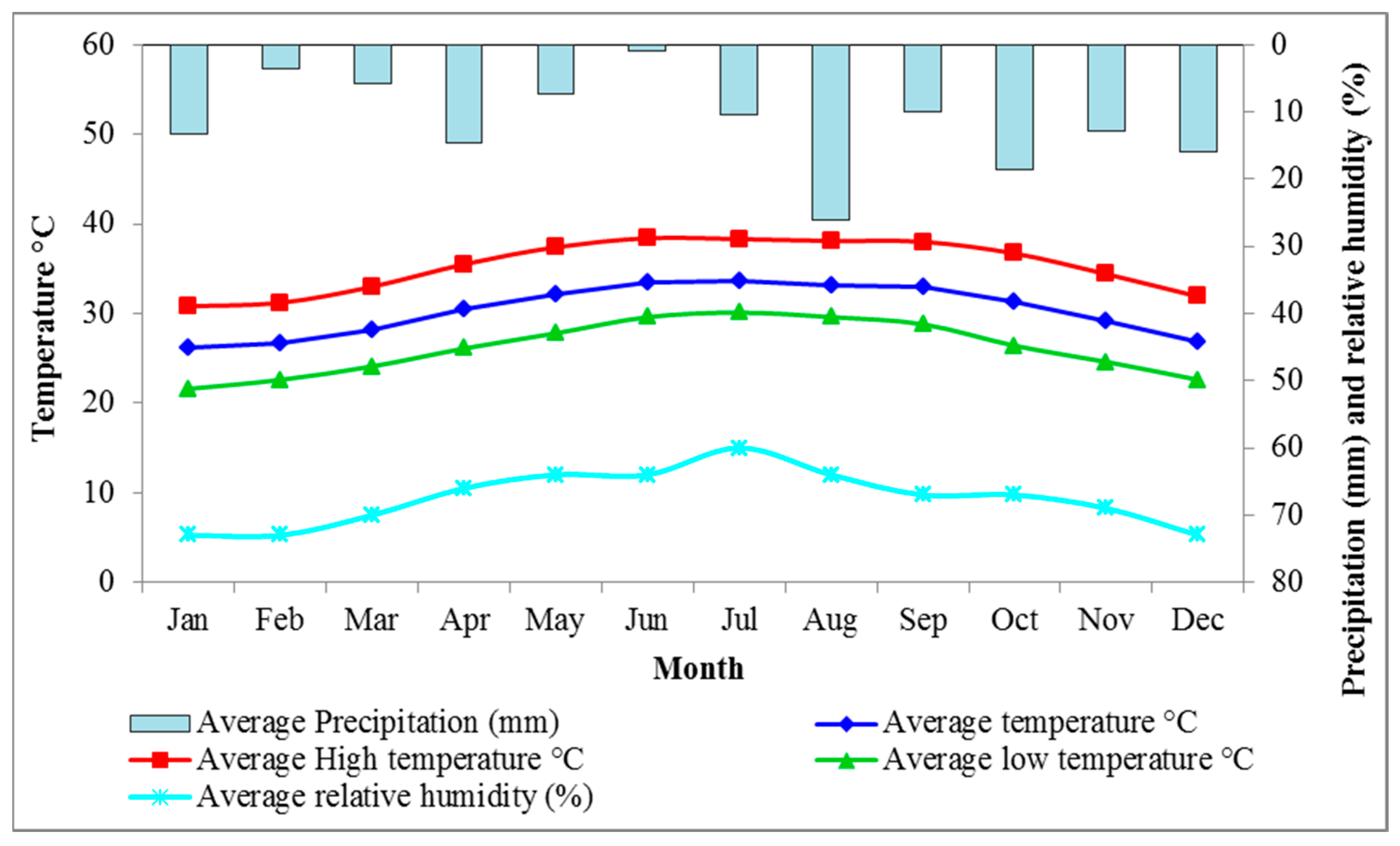
The Jizan study area is located in the southwest corner of Saudi Arabia, directly north of the border with Yemen. It is located between longitude 41°56′18″ E and 43°15′58″ E and latitude 16°23′8″ N and 17°53′56″ N (Figure 1). The study area covers about 10,753 km2. Jazan City is located on the Red Sea coast and serves a large agricultural heartland with a population of 319,119 as of 2021. Based on climate data for Jazan from 1985 to 2010 (Figure 2), Jazan has a hot desert climate with an average annual temperature of more than 30 °C. The weather is extremely hot all year, with daily lows averaging over 25 °C and highs averaging over 35 °C even in the coldest month. The average evaporation rate is 2000 mm/year (Source: Jeddah Regional Climate Center [38]. The southwestern region of Saudi Arabia is rich in rainfall compared to other areas of the Kingdom of Saudi Arabia, with average annual precipitation in the range of 400–700 mm/year [39]. The watersheds collect these precipitations that exclusively occur during the winter season from the adjoining hills and channel the collected runoff toward the Red Sea as surface runoff and/or infiltration into the near-surface aquifers [40,41]. The importance of the study area for national and economic development was a driving goal for this research.
The study area spans the western margin of the Proterozoic Arabian Shield and the eastern margin of the Cenozoic Red Sea basin. The Cenozoic rocks are represented by the clastic sedimentary succession underlying the black basaltic sheet of lava flows. The Quaternary deposits cover about half of the Jazan area in the wadi beds and the coastal plain. They consist of interbedded clay and sands, silts, cobbles, and gravels of wadi beds with variable thicknesses from one place to another. The thickness of the alluvial sediments ranges from 10 m towards the foothills to more than 100 m distant from the highlands in the southwest parts [2,42].

2.2. Dataset Collection

A total of 145 groundwater samples were collected and chemically analysed from both shallow dug wells and boreholes tapping the phreatic aquifer (Figure 1). Collected water samples were analysed for major cations (Ca2+, Mg2+, Na+, K+) and anions (HCO3, SO42, Cl, CO32−) by following standard methods suggested by APHA American Public Health Association (APHA) [43]. Table 1 displays descriptive statistics for physicochemical variables of the groundwater samples and the maximum permissible limits for various parameters, according to the WHO [44]. The inverse distance weighted (IDW) interpolation in GIS was used to map the spatial distribution of the chemical water parameters.

2.3. Water Quality Index (WQI)

This study uses eleven water quality parameters to calculate a WQI based on the World Health Organization’s recommended drinking water quality standards (WHO) [44]. The WQI was analysed using the physicochemical parameters of pH, TDS, Ca2+, Mg2+, Na+, K+, Cl, SO42−, HCO3, NO3, and TH. The weighted arithmetic WQI (WAWQI), proposed by Horton [37], was used to assess the water quality.
W A W Q I = i = 1 n W i Q i
where Wi is the relative weight of each parameter (Equation (2)), and Qi (Equation (3)) is the quality rate scale assigned to each parameter by dividing the parameter concentration of the water sample by its respective standard as per the WHO guidelines [44] (Table 1).
W i = w i i = 1 n w i
Q i = C i S i
where wi is the weight of each parameter on a scale of one to five, indicating their relative relevance for drinking water quality, n is the number of parameters, Ci and Si are respectively the concentration of parameter i, and the standard value of parameter i. Table 2 shows the weights for the various water parameters [33]. Table 3 shows the classification of water quality according to the WAWQI type and range.

2.4. Machine Learning Methods

2.4.1. Multiple Regression

The input parameters of the ANN model were determined using the multiple linear regression model [46]. The purpose of multiple linear regression analysis is to use known independent variables to predict the value of a single dependent variable. The weights of each predictor value indicate how big of an impact it has on the total projection. The independent variables are water quality measures (X1, X2,..., Xn) for the dependent WAWQI in this study (Y).
Y = a 0 + a 1 X 1 + a 2 X 2 + a 3 X 3 + + a i X i + + a n X n
where Xi: is the dependent variable i; n is the number of the dependent variables, ai is the ith coefficient of the dependent variable Xi, a0 is the constant term of the model.

2.4.2. Artificial Neural Network (ANN)

ANNs were used to predict the WAWQI using MATLAB’s Neural Network library (MathWorks, Natick, MA, USA). The ANN model’s input, hidden, and output layers are all separate layers, and each layer contains different types of neurons. The input parameters are entered into the network and stored in input neurons, while the calculated outcomes are attributed in the output layer by output neurons. The hidden layer acts as a mediator to connect the input and output layers [47]. There are many different types of ANNs; one of the most common is the Bayesian regularisation back propagation (BRBP), which is the type applied in this research. The BRBP is a network training function that uses Levenberg Marquardt optimisation to update weight and bias variables. It finds the best mix of squared errors and weights to construct a network that generalises well [48,49].
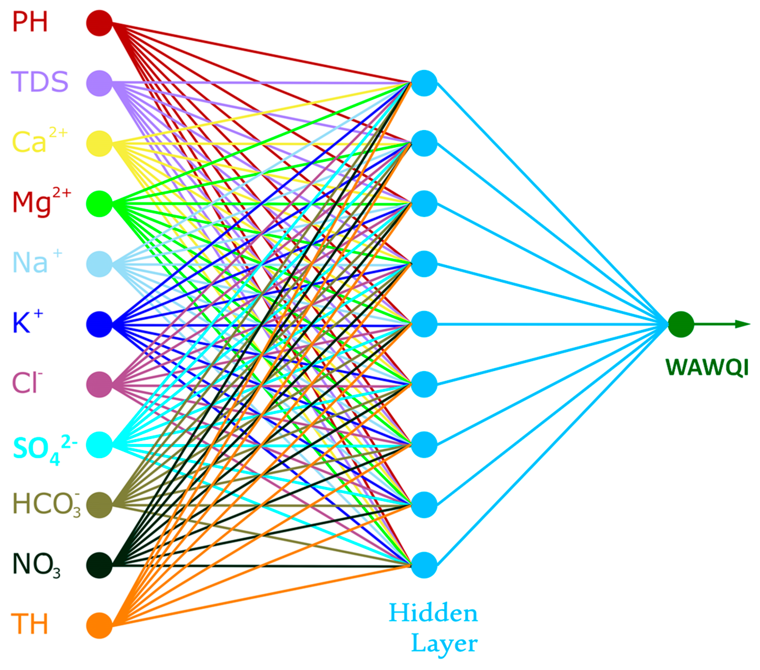
The input parameters of the ANN model in this work were 11 input neurons, which included physicochemical parameters such as pH, TDS, Ca2+, Mg2+, Na+, K+, Cl, SO42−, HCO3, NO3, and TH, while the output neurons were the WAWQI (Figure 3). In the hidden layer, nine neurons were used. Moreover, 75% of the dataset was allocated for training the models, and the remaining were considered for testing and validating the models.

2.4.3. Support Vector Machines (SVM)

SVM analysis is a common machine-learning tool for regression analysis and classification [50]. Because it uses kernel functions, SVM regression is classified as a non-parametric approach. The SVM model is used to improve accuracy on low to medium-dimensional data sets. SVM regression is used to find the linear function for training data x of N observations with observed response values y.
f x = y = w b T x 1 = w T x + b x , b R N + 1
where the parameters w and b are the gradient and the intercept, respectively, and ε represents the tolerance margin, as shown in Figure 4.
The kernel function determines the non-linear transformation applied to the data before the SVM is trained. In this paper, linear and polynomial kernel functions are used. The memory usage for cubic SVM is higher than linear SVM [52]. The Machine Learning Toolbox in MATLAB provides the following linear and polynomial kernel functions:
Linear : G x i , x j = x i x j
Polynomial :   G x i , x j = ( 1 + x i x j ) q , w h e r e   q   i s   i n   t h e   s e t   { 2,3 , 4 , }
The Gram matrix is an n-by-n matrix with entries gi,j = G(xi,xj). Each element gi,j represents the inner product of the predictors as transformed by φ. However, no need to know φ; the Gram matrix can be directly constructed using the kernel function. Non-linear SVM uses this method to determine the best function f(x) in the altered predictor space. In this paper, x represents the input vector (11 physicochemical parameters), f(x) refers to WAWQI, and in the polynomial kernel function, q was set as 3 (cubic).

2.4.4. Fit Binary Tree

A binary search tree (BST), also known as an ordered or sorted binary tree, is a rooted binary tree data structure in which each internal node stores a value that is higher than all keys in the node’s left subtree but less than those in the node’s right subtree. The temporal complexity of operations on the binary search tree is related to the tree’s height. Binary search trees provide a binary search for quick data lookup, addition, and removal and may be used to construct dynamic sets and lookup tables. Because the nodes in a BST are arranged so that each comparison skips around half of the remaining tree, the lookup performance is proportional to that of the binary logarithm. In BST, the left sub-tree has elements less than the nodes element, and the right sub-tree has elements greater than the nodes element. A data structure called a BST makes it easy to keep track of a sorted list of numbers. Because each tree node can only have two children, it is known as a binary tree. Because it may be used to search for the presence of a number in O(log(n)) time, it is known as a search tree. BST is a node-based binary tree data structure that has the following properties: The left sub-tree of a node contains only nodes with keys lesser than the node’s key; The right sub-tree of a node contains only nodes with keys greater than the node’s key; The left and right sub-tree each must also be a binary search tree; there must be no duplicate nodes. Data representation is carried out in the ordered format, and BST does not allow duplicate values. The performance of a binary search tree is determined by the sequence in which the nodes are inserted into the tree; various binary search tree versions may be made with assured worst-case performance. The fundamental operations are search, traverse, insert, and delete. BSTs with assured worst-case complexity outperform an unsorted array, which would need a linear search time. The following pseudocode recursively implements the BST search method (Algorithm 1).
Algorithm 1. Pseudocode recursively for the BST search method.
Tree-Search(x, key)
 if x = NIL or key = x.key then
  return x
 if key < x.key then
  return Tree-Search(x.left, key)
 else
  return Tree-Search(x.right, key)
 end if
The recursive procedure continues until a NIL is reached or the observed and simulated values are in good agreement.

2.4.5. Gaussian Process Regression (GPR)

The GPR mathematical model is a non-parametric kernel-based probabilistic model [53]. It is important in the field of machine learning programming. The essential understanding of GPR is that the learning sample tracks the past probabilities of the Gaussian process regression. It is based on calculating the consistent subsequent probability and is built using the Bayesian linear regression model. GPR uses the kernel to define the covariance of a prior distribution across the target functions, and the observed training information is used to explain a likelihood function. Based on the Bayes theorem, a (Gaussian) posterior circulation across goal functions is explained, and its mean is used for data prediction. GPR was originally proposed as a ‘principled, practically, and probabilistically based approach to kernel-making’ [53]. The benefit of GPR over many other methods is that it smoothly integrates hyper-parameter estimates, model training, and risk evaluations; the results are less subjectively impacted and more understandable as a consequence. Gaussian processes (GP) are based on the assumption that the combined dispersion of model output probability is Gaussian [54].
Polynomial kernel (poly kernel) is a kernel feature that is commonly employed with the GPR in the initial variables of a function space to develop non-linear models. The polynomial kernel emerges automatically at the defined characteristics of the input samples to acquire their likeness, as well as combinations of them. In the context of regression analysis, such groups are referred to as interactive features. The enclosed polynomial kernel feature space is similar to a polynomial regression, but it is an educated sum of parameters that do not have a combinative blow-up. When the features’ input data is binary (boolean), the features are linked to logical input function conjunctions [55].
The polynomial kernel is well-defined as follows:
K x , Y = ( x T ,   y   +   C ) d
where x and y are vectors in the input space, i.e., vectors of features estimated from workout or trial samples, and C ≥ 0 is an unlimited parameter balancing the approach of higher-order vs. lower-order polynomial formulations. When C equals zero, the kernel is said to be homogenous.

2.5. Evaluation Indicators

Five statistical indicators were used to assess the performance of the linear regression, ANN, and SVM models: mean error (ME), mean absolute error (MAE), root mean square error (RMSE), mean absolute percentage error (MAPE), coefficient of correlation (R), and R-squared. The following equations were used to determine these indicators:
M E = 1 N i = 1 N Y i Y i *
M A E = 1 N i = 1 N Y i Y i *
R M S E = 1 N i = 1 N Y i Y i * 2
M A P E = 1 N i = 1 N Y i Y i * Y i * × 100
R = I = i N Y i Y ¯ Y i * Y * ¯ i = 1 N Y i Y ¯ 2 i = 1 N Y i * Y * ¯ 2
where N is the number of measurements, Yi is the measured value for each parameter, Y* is the estimated value for each parameter, Y ¯ is the mean of the measured values of the Y variables, and Y * ¯ is the mean of the estimated values of Y* variables.

3. Results and Discussion

3.1. Hydrogeological Aspects

The hydrogeological conditions have been studied in the Jazan area, where the groundwater is stored in both the alluvial deposits of the wadi systems and the clastic coarse members of the Cretaceous–Tertiary sedimentary succession [56]. The alluvial aquifer is composed of the Quaternary wadi deposits that enhance seawater intrusion in the coastal aquifer [2,57]. The aquifer’s transmissivity ranges from 540 to 5400 m2/day, with an average of 2190 m2/day, and specific yield ranges between 0.001 and 0.006, increasing towards west directions, indicating good productivity. The storativity coefficient ranges between 0.01 and 0.25, with an average of 0.13 increasing toward the west direction [58]. Uncontrolled pumping in many locations has caused a cone of depression with the inland movement of the seawater fronts. The main recharge components of the aquifer are local rainfall infiltration that exclusively occurs during floods in the winter season. The shallow unconfined aquifer is subject to over-exploitation from many scattered wells in the area. Discharge of the aquifer includes groundwater pumping from wells to provide an adequate water supply for agricultural and residential areas and evapotranspiration losses in places where the water table is close to the ground surface [2].
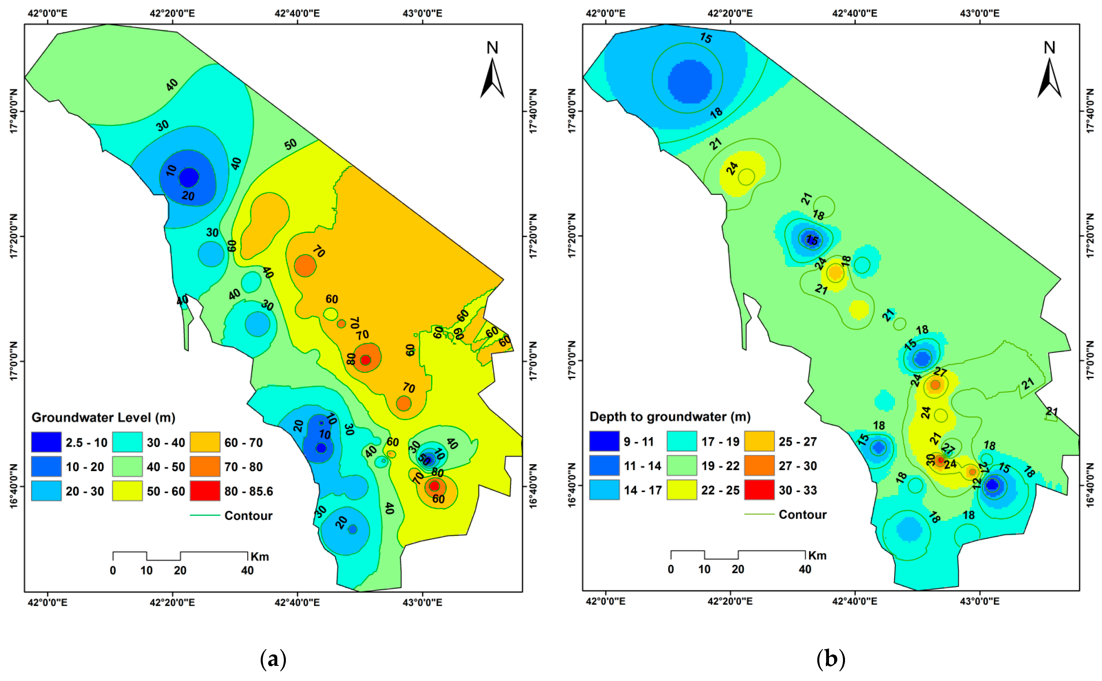
Figure 5 shows the hydrogeological conditions ascertained from the fieldwork, including groundwater level compared with the mean sea level (m.asl) and depth of groundwater in the study area. Groundwater occurs at shallow depths, where groundwater levels vary from 10 to 33 m below the ground surface (Figure 5b). The piezometric gradient is inclined towards the west and southwest direction; it varies from 0.005 in the upper parts of the wadi to 0.001 at the beginning of the coastal plain [2]. Generally, the groundwater flow is from the east and northeast to the west and southwest toward the sea (Figure 5a); this might be due to the positive hydraulic gradient set up by the balance between recharge inland and discharge toward the sea. However, excessive fresh groundwater pumping in many areas causes a modification of the natural flow systems (reversing the hydraulic gradients) and, thus, induces seawater intrusion. However, few areas showed characteristic cones of depression.

3.2. Statistical Analysis

Table 4 presents the descriptive statistics for the 145 water quality samples. Moreover, the correlation matrix is useful since it independently illustrates each parameter’s importance and its effect on the hydrochemical relationships. If (r) values in Pearson’s correlation matrix (Table 5) are +1 or −1, they represent a complete correlation between two variables, i.e., functional dependence. If the values are near zero, there is no significant interaction between the two variables at the p < 0.05 level.

3.3. Chemical Analysis, Spatial Distribution, and Correlation Coefficients

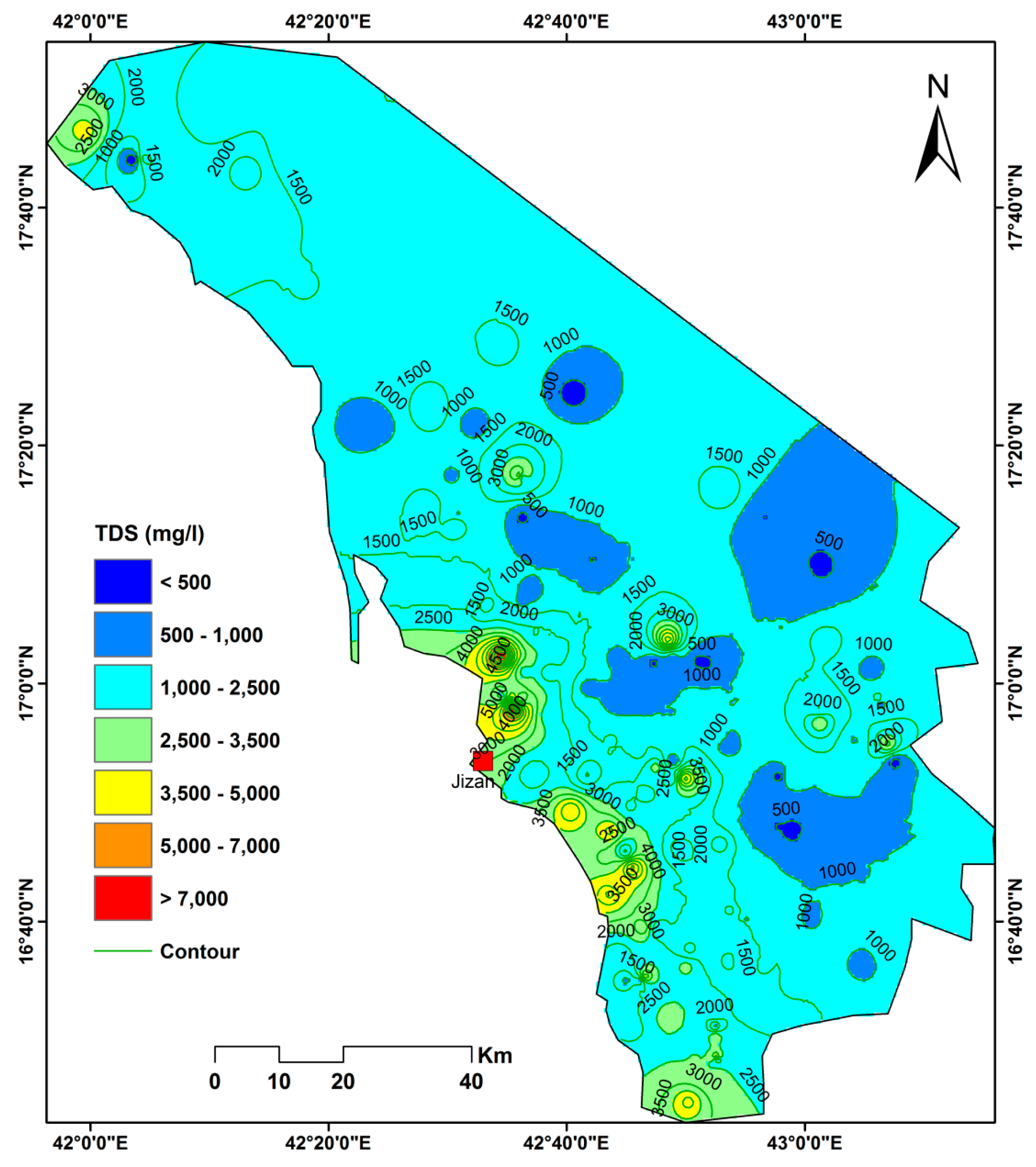
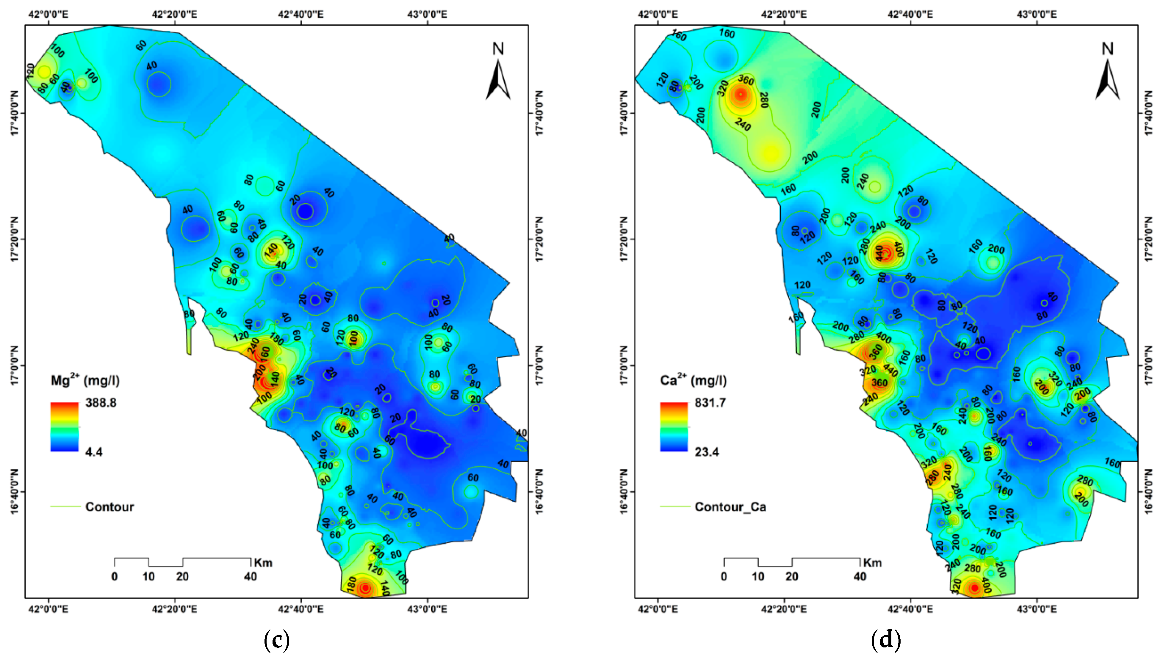
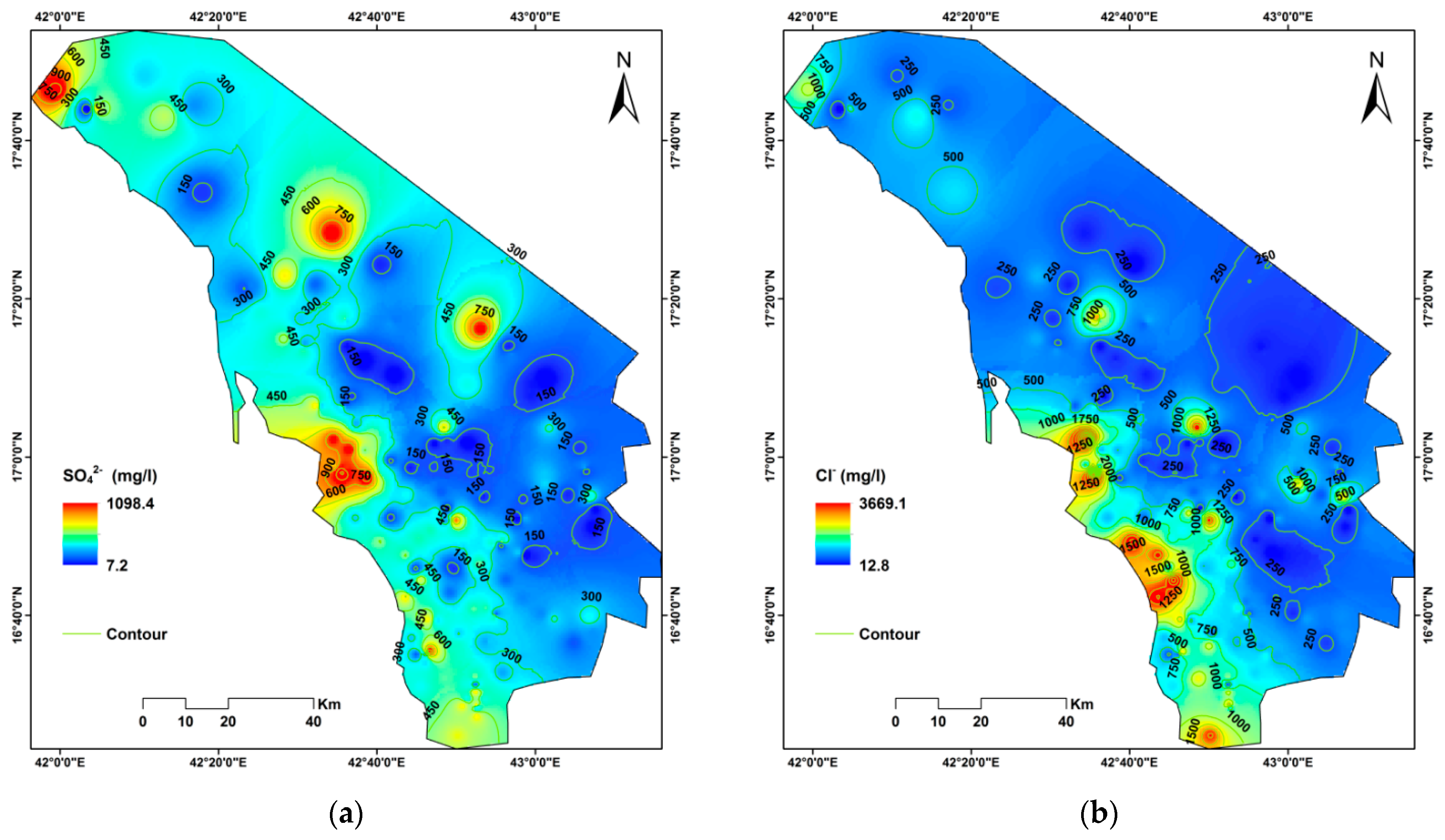
The results of the chemical analysis indicated that the dominant cations are Na+, followed by Ca2+ and Mg2+, while the dominant anions are Cl followed by SO42− and HCO3, with a minor contribution of NO3. Cations and anions reflect sodium chloride water type (Table 1). The pH of the groundwater ranges between 6.33 and 8.68, with an average of 7.66 indicating more or less neutral groundwater that is generally suitable for drinking. TDS is an important parameter for assessing salinity hazards and suitability for drinking and irrigation. The TDS ranges from 128 mg/L in the boreholes located further inland to 8320 mg/L close to the coastline, with an average of 1709 mg/L; thus, a wide range of variation was detected (Figure 6). The higher TDS values are recorded in groundwater wells near the Red Sea coast, indicating significant groundwater salinisation due to seawater intrusion. This seawater intrusion in the coastal aquifer of Jazan was confirmed by Abdalla [42], Abdalla et al. [2], Al-Bassam and Hussein [57].
The increase of Ca2+ and Mg2+ concentrations with the increasing salinity could indicate reverse ion exchange in the aquifer. High Cl and SO42− concentrations were recorded in places close to the coastline and indicate seawater intrusion.
The spatial distribution of the major cations (K+, Na+, Mg2+, Ca2+) and major anions (SO42–, Cl, HCO3, NO3) is shown in Figure 7 and Figure 8, respectively.

3.4. Water Quality Index Distribution and Classification

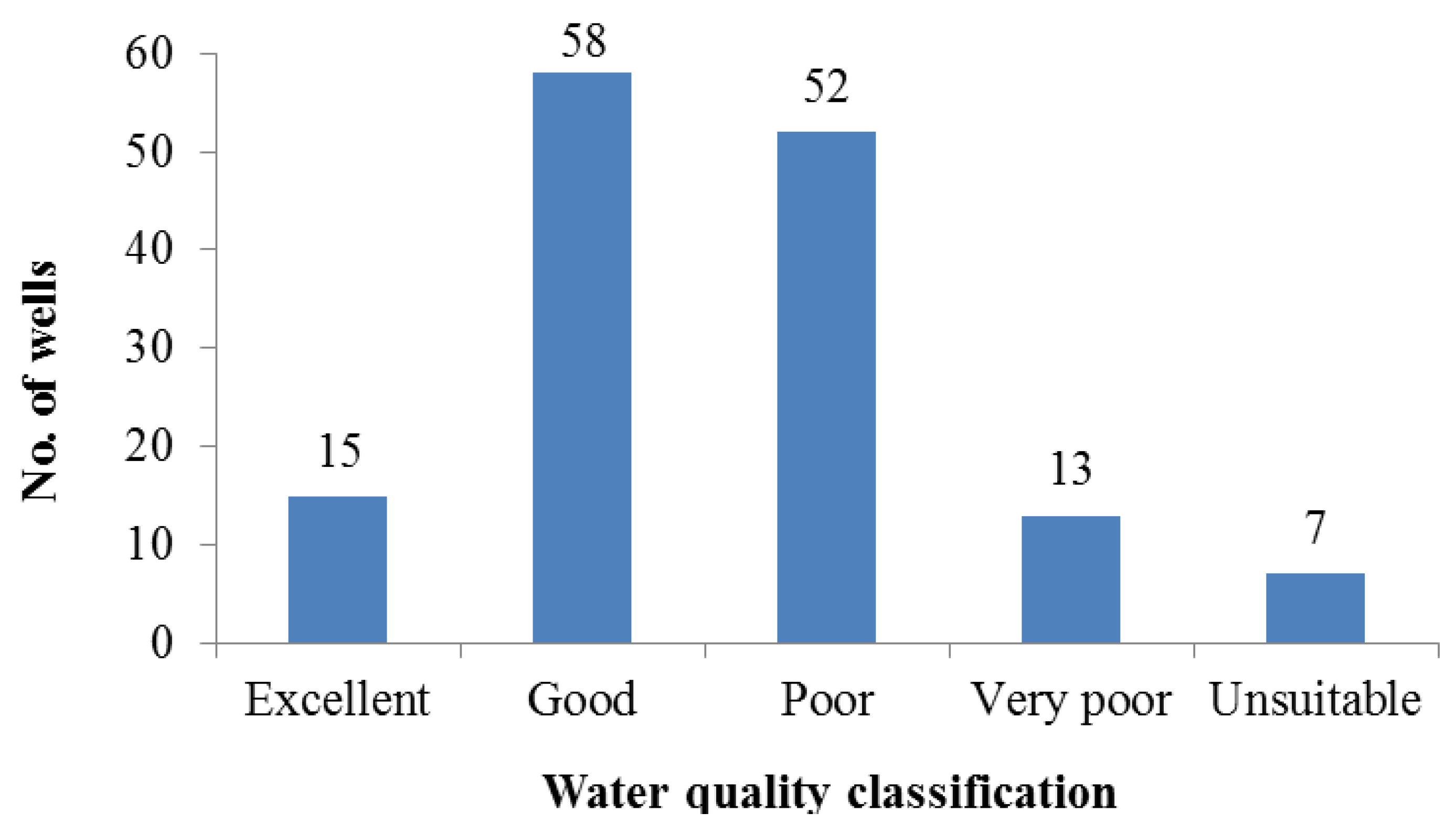
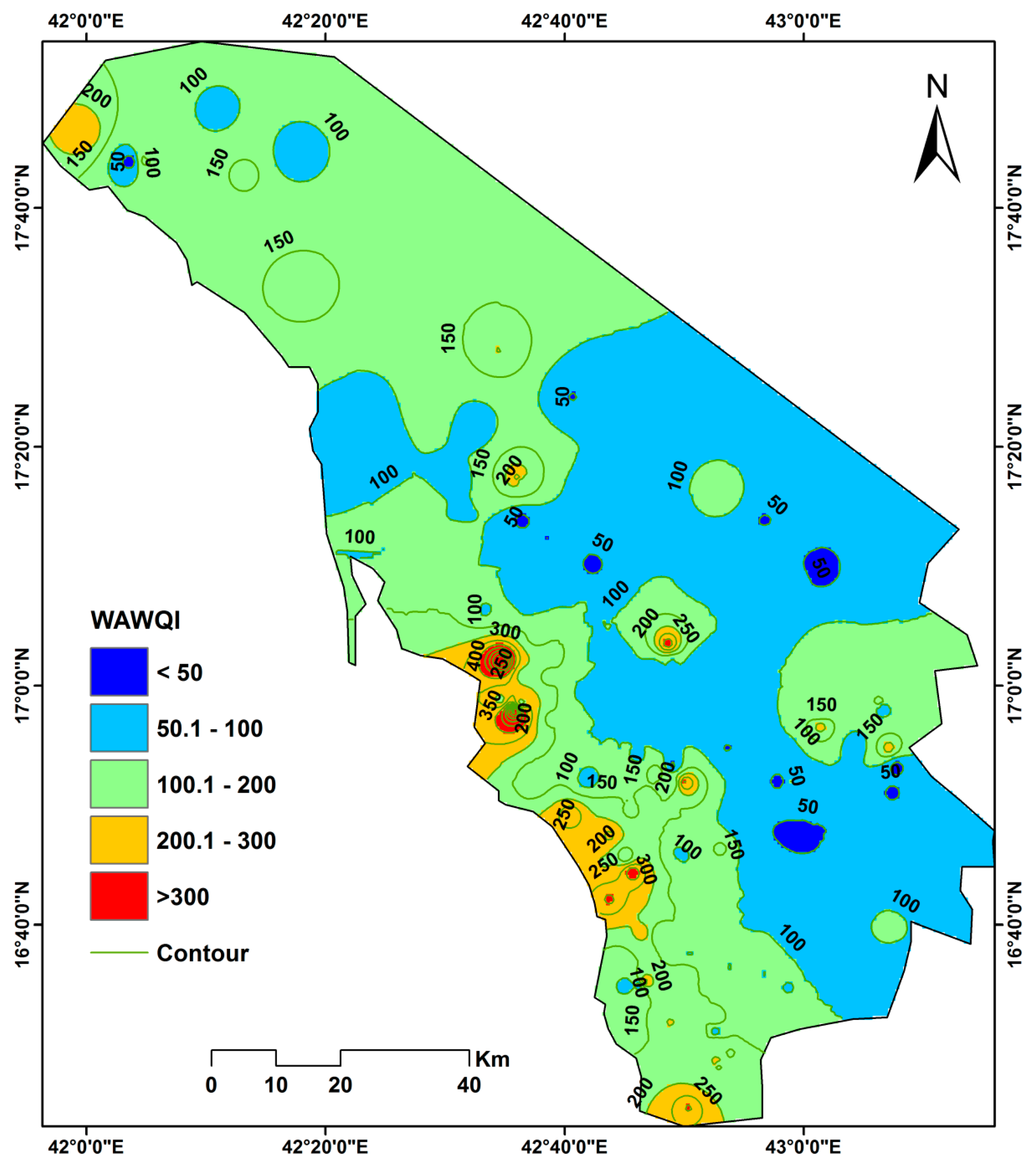
The calculated WAWQI shows that 15 wells have a score of less than 50, indicating excellent water quality, according to Kumar et al. [45] (Table 3). The WAWQI of 58 wells ranges from 50.1 to 100, indicating good quality water. Figure 9 depicts the WQI classification: 52 wells have a WQI of 100.1–200, indicating water of poor quality, and 13 wells have a WQI of 200.1–300, indicating water of extremely poor quality. Finally, seven wells have a WQI of greater than 300, indicating that the water is unfit for consumption. The spatial distribution of the WQI over the region is depicted using inverse distance weighted (IDW) interpolation in Figure 10.

3.5. Evaluation of Data-Driven Models in WQ Prediction

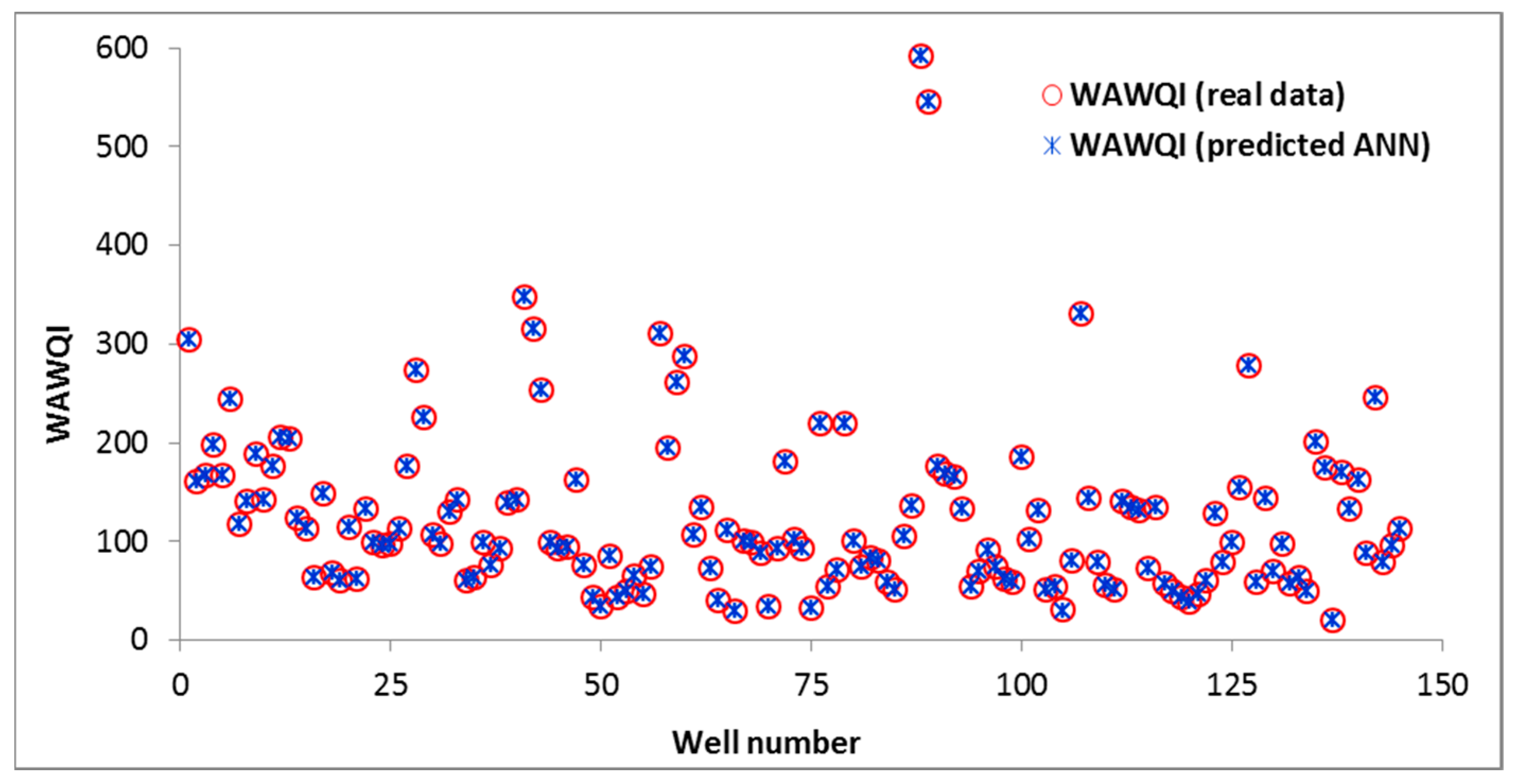
The data were fitted using stepwise regression for the linear regression model, which produced a model that closely matched the observed and predicted WAWQI values. The input data were first structured as a dataset array, and the response data (WAWQI) were then arranged as a column vector. Each row of input data represents one observation. The regression model is then developed. The stepwise fit model begins with a single model, such as a constant, and then adds or subtracts terms one by one. Then, in a greedy manner, it selects an ideal parameter each time until it can no longer improve. The data should then be checked for outliers. The model coefficients obtained from the linear regression model are presented in Table 6. The model findings for this case study show that pH, K+, and NO3 are the most significant variables and HCO3 is considered an insignificant variable. The model appears as in Equation (14). R2 = 1 indicates that the data fit the model well. The MSE is 0.003, and the RMSE is 0.0023. Figure 11 shows the comparison of predicted and measured WAWQI.
W A W Q I = 0.0057308 + 1.4292 p H + 0.069523 T H 0.098639 C a 2 + + 0.025649 M g 2 + + 0.050002 N a + + 0.41667 K + + 0.050032 C l + 0.0071646 H C O 3 + 0.03574 S O 4 2 + 0.24998 N O 3
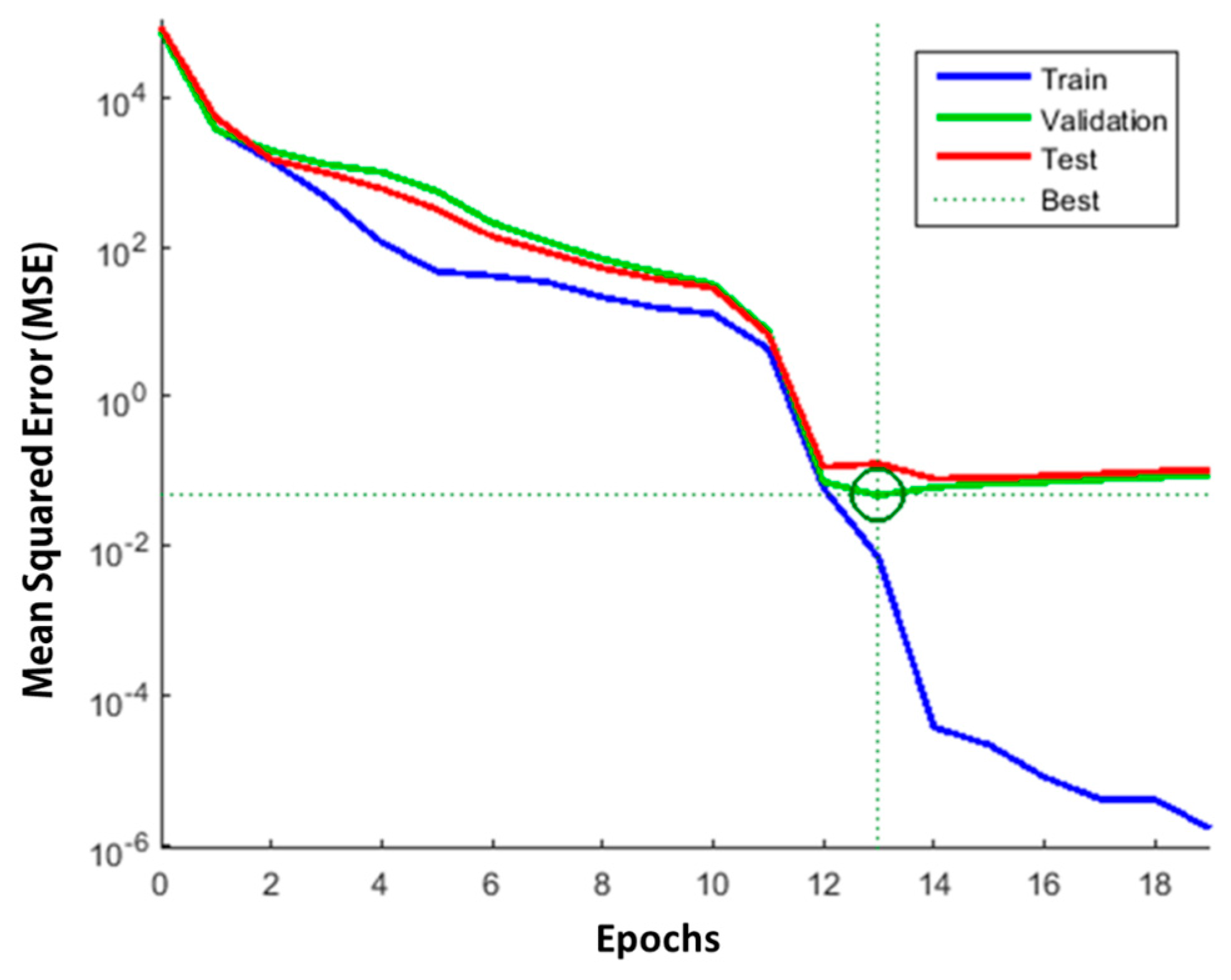
The best result for the ANN modelling was obtained for the network with nine neurons after 19 iterations, while the best validation result was displayed for the network after 13 iterations (Figure 12).
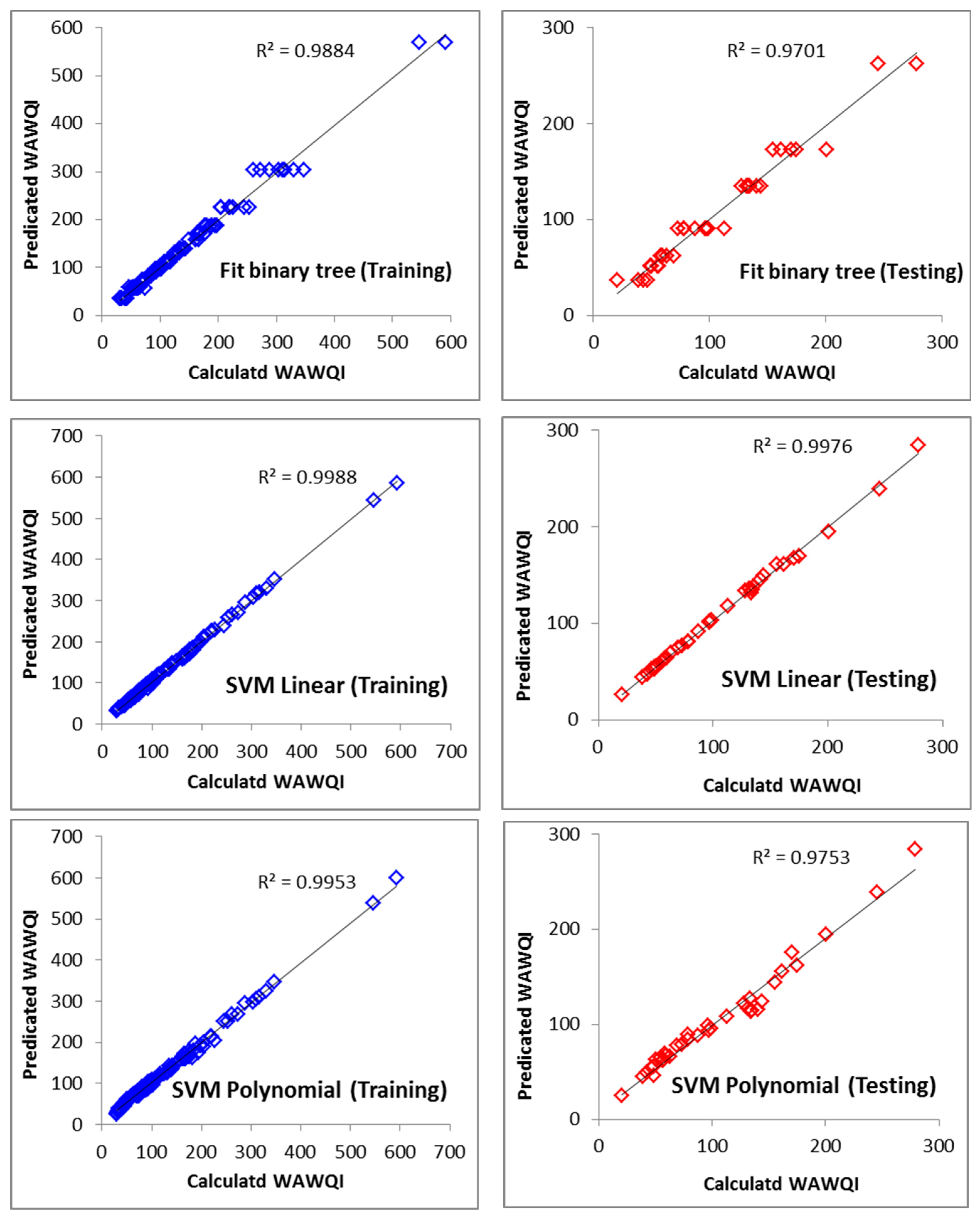
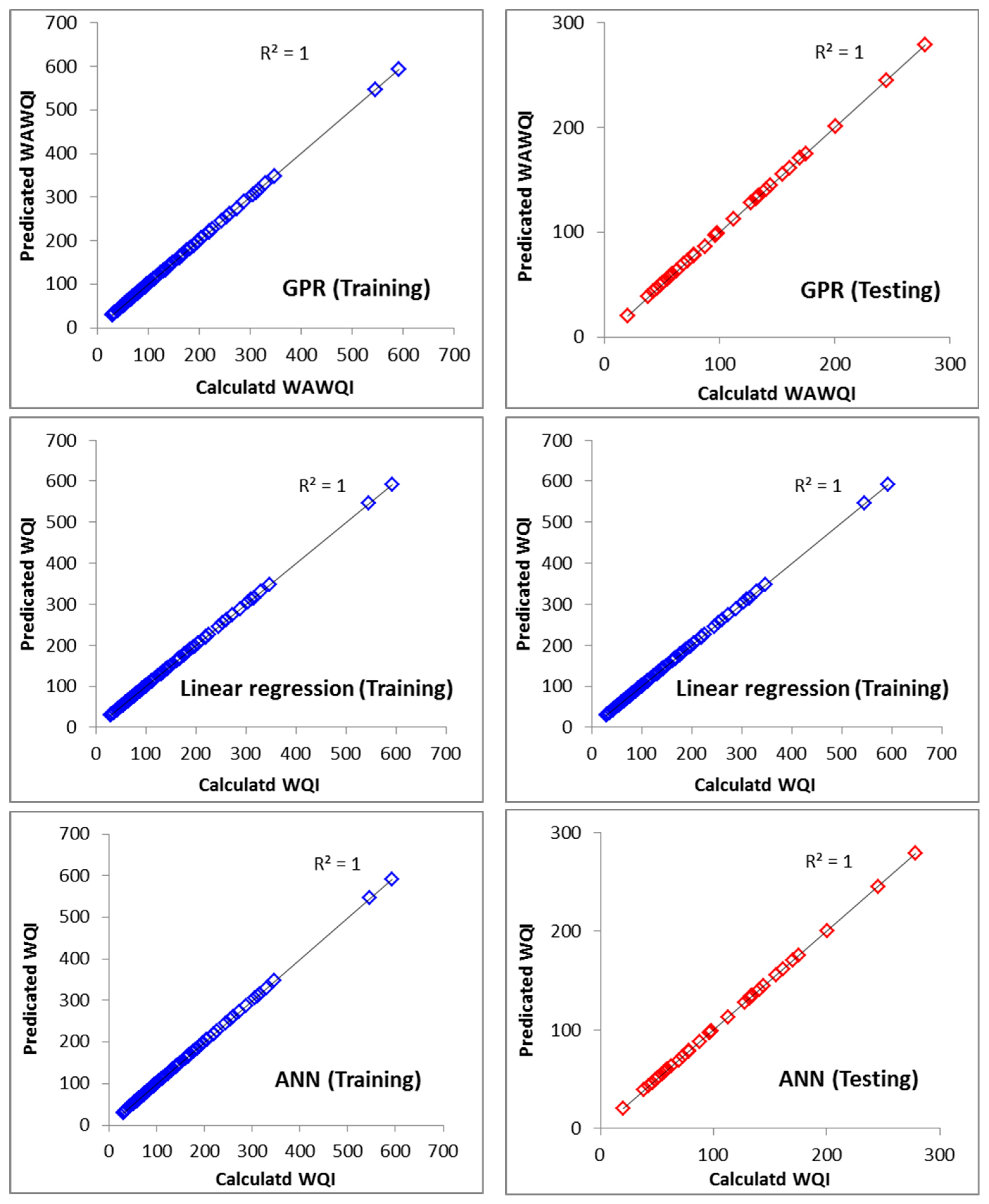
The ME, MAE, RMSE, MAPE, regression factor R, and R2 were used to validate the applied models’ performance (Table 7). The scatterplots of the predicted and calculated WAWQI for the applied models in the training stage (right) and testing stage (left) are shown in Figure 13.
The GPR, linear regression (stepwise), and ANN models all worked perfectly in the training and testing phases, as shown in Table 7. In both phases, these models had a high correlation, nearly to one, and small statistical errors. The linear regression (stepwise) model produced the best results, with MAE = 0.0023, RMSE = 0.0028, MAPE = 0.0025%, R = 1.0, and R2 = 1.0. The ANN model came in second with MAE = 0.088, RMSE = 0.0884, MAPE = 0.0969%, R = 1.0, and R2 = 1.0. At the same time, the GPR model came in third with MAE = 0.194, RMSE = 0.255, MAPE = 0.234%, R = 1.0, and R2 = 1.0. This was followed by the SVM (Linear) model with MAE = 3.39, RMSE = 3.83, MAPE = 3.38%, R = 0.9988, and R2 = 0.9994. The SVM (Gaussian kernel) and Fit binary tree models performed the worst in the training and testing phases of the prediction procedure. For the SVM (polynomial kernel) model, the MAE, RMSE, MAPE, R, and R2 were 6.42, 8.14, 5.45%, 0.9953, and 0.9976, respectively. For the Fit binary tree, the MAE, RMSE, MAPE, R, and R2 were 6.07, 10.09, 4.92%, 0.9884, and 0.9942, respectively (Table 7).
Overall results showed that the proposed methods generated satisfactory outputs for estimating WAWQI close to observed data. The results obtained are highly satisfactory compared with the findings from Sakaa et al. [59], who showed that a combination of all input parameters attained a best predictive performance of R2 testing = 0.82, RMSE testing = 5.17, while a couple of five input parameters, such as pH, EC, TDS, T, and saturation, achieved the second-best predictive precision (R2 testing = 0.81, RMSE testing = 5.55). In addition, the current findings are in agreement with the results of Mokhtar et al. [27], who used SVM, extreme gradient boosting, Random Forest and stepwise regression, principal components regression, partial least squares regression, and ordinary least squares regression for WQI modelling and stated that all models used with values less than 0.1 show good prediction ability for all indices. These findings were extremely acceptable and agreed with those suggested by Elbeltagi et al. [60], who applied additive regression (AR), M5P tree model (M5P), random subspace (RSS), and SVM in WQI modelling and found that AR outperformed the other data-driven models (R2 = 0.9993, MAE = 0.5243, RMSE = 0.06356, RAE% = 3.8449, and RRSE% = 3.9925). The AR was offered as an optimal model with good outcomes due to improved prediction precision with the fewest input parameters. Moreover, eight artificial intelligence algorithms, e.g., multi-linear regression (MLR), random forest (RF), M5P tree (M5P), random subspace (RSS), additive regression (AR), artificial neural network (ANN), support vector regression (SVR), and locally weighted linear regression (LWLR) have been applied by Kouadri et al. [35]. Their results stated that the MLR model performed better than the other models, whereas the RF model performed better. Also, the model results coincide with Kouadri et al. [36], who implemented long short-term memory (LSTM), multi-linear regression (MLR), and ANN and stated that the results are highly accurately predicted using ANN and MLR models compared to LSTM model. These models also generated more favourable outcomes than those achieved by Iqbal et al. [61], who used the WASP8 for water quality simulations. Their results clarified that Pearson correlation coefficient values are around 0.66, 0.68, and 0.58, respectively.

3.6. Best Subset Regression for Selecting the Most Important Parameters

Feature selection is one of the most important stages in a soft computing model to forecast and predict phenomena with many input variables. There are several approaches to specify the best combinations among all possible, including best subset regression, mutual information, and forward stepwise selection. The best subset regression analysis was performed in the current study to determine the best input combinations for the WAWQI model. For this purpose, six statistical criteria, including MSE, determination coefficients (R2), adjusted R2, Mallows’ Cp, Akaike’s AIC, and Amemiya’s prediction criterion (PC), were computed, and the results are shown in Table 8. As can be seen, the eight bold input combinations have the lowest values of Amemiya’s PC (from 0.00 to 0.027) among all input combinations. These eight input combinations have a high R2 (from 0.975 to 1.00) and high Adj-R2 (from 0.974 to 1.00) and were identified as the best input combination for the prediction of the WAWQI model. It is noteworthy that a total of 145 datasets were randomly split into two training and testing subsets. Moreover, 75% of the datasets were allocated for training the models, and the remaining were considered for testing and validating the models.

4. Conclusions and Outlook

This study analysed the ability of six different AI techniques and regressions, such as linear regression (stepwise), support vector regression SVM (linear and polynomial kernels), Gaussian process regression (GPR), Fit binary tree, and artificial neural network ANN (Bayesian) for forecasting a WQI based on 11 physicochemical parameters (pH, TDS, Ca2+, Mg2+, Na+, K+, Cl, SO42−, HCO3, NO3, and TH) collected from 145 groundwater wells in Jizan, Saudi Arabia.
The outcome of the resultant WQI model clearly identified (forecasted and predicted) the best input combination for the prediction of the WAWQI model. This might contribute significantly to the knowledge and understanding of the groundwater quality within the study area and its impact on any agricultural investments and sustainable development, as the study area has high importance to national and regional economic development especially agricultural and industrial activities.
In addition, ArcGIS was used to create maps of the spatial distribution of groundwater quality parameters. The best subset regression analysis was used to find the optimum input combinations for the WQI model.
The following findings have been obtained:
-
Higher levels of Cl and SO42− were found near the coast, which is indicative of seawater intrusion and serves as a proxy for salinisation. Furthermore, seven wells had a WAWQI of more than 300, suggesting that the water is unsafe for human consumption.
-
The results of the stepwise fit model revealed that pH, K+, and NO3 are the most important variables, while HCO3 is a non-significant variable. The best results were obtained from the simulated ANN modeling for the nine-neuron network after 19 iterations, whereas the best validation performance was 0.048016 at iteration 13.
-
The GPR, linear regression (Stepwise), and ANN models worked flawlessly during the training and testing stages, with a high correlation of 1 and low statistical errors.
-
The linear regression (stepwise) model generated the best results, with MAE = 0.0023, RMSE = 0.0028, and R = 1.0. This good performance is due to its special mechanism with repeated regressions, each time deleting the weakest associated variable until the observed and measured values fully match. The ANN model came in second with MAE = 0.088, RMSE = 0.0884, and R = 1.0. The GPR model finished in third with MAE = 0.194, RMSE = 0.255, and R = 1.0. The SVM (Linear) model was next, with MAE = 3.39, RMSE = 3.83, R = 0.9988.
-
The SVM (polynomial kernel) and Fit binary tree models performed the worst during the training and testing phases of the prediction procedure.
-
The optimum input combination for WAWQI model prediction was the eight input combinations with high R2 (from 0.975 to 1.00) and high Adj-R2 (from 0.974 to 1.00).
These findings are of importance to water planners in terms of WQI for enhancing sustainable groundwater resource management policies.
In conclusion, the best subset regression analysis is useful, and when only a portion of the relevant data are available, we can use the best subset regression model to determine which input parameters will best match the ML model for WQ prediction.
This study recommends not using SVM (polynomial kernel) and Fit binary tree models because of performing the worst during the training and testing phases of the prediction procedure. It can be recommended, in future works, standalone and hybrid artificial intelligence models for predicting WQIs in several regions under different conditions should be developed to recommend which model is most suitable for all these regions based on limited input variables. Future research can also incorporate depth to groundwater variation data into AI/ML methods to investigate its effects on groundwater quality. It is also recommended that seawater intrusion be controlled in the study area by implementing one of the following techniques: decreasing pumping rates, hydraulic barriers, artificial recharge using treated wastewater [62,63,64], using a freshwater surface recharge canal [65], cutoff walls [66,67], and brackish water pumping [68].

Author Contributions

Conceptualization, M.E.-R.; methodology, M.E.-R., O.B. and A.E.; software, M.E.-R.; validation, M.E.-R. and A.E.; formal analysis, M.E.-R. and A.E.; investigation, M.E.-R.; resources, M.E.-R.; data curation, M.E.-R.; writing—original draft preparation, M.E.-R. writing—review and editing, M.E.-R., O.B., F.A., S.A., M.S.A. and A.E.; visualization, M.E.-R. and A.E. All authors have read and agreed to the published version of the manuscript.

Funding

This research was funded by the Deputyship for Research and Innovation, Ministry of Education in Saudi Arabia, project no. (IFKSURC-1-7314).

Data Availability Statement

Data available based on request from first author.

Acknowledgments

The authors extend their appreciation to the Deputyship for Research & Innovation, Ministry of Education in Saudi Arabia, for funding this research. (IFKSURC-1-7314).

Conflicts of Interest

The authors declare no conflict of interest.

Abbreviations

AdaBoostAdaptive Boosting
AIArtificial Intelligence
ANNArtificial Neural Network
APHAAmerican Public Health Association
ARAdditive Regression
BRBPBayesian Regularisation Back Propagation
BSTA Binary Search Tree
Ca2+Calcium Ion
CCMEWQICanadian Council of Ministers of the Environment Water Quality Index
ClChlorine Ion
GAGenetic Algorithms
GISGeographic Information System
GPRGaussian Process Regression
HCO3Bicarbonate Ion
IDWInverse Distance Weighted
IWQIrrigation Water Quality
K+Potassium Ion
kNNK-Nearest Neighbour
LSTMLong Short-Term Memory
LWLRLocally Weighted Linear Regression
MAEMean Absolute Error
MAPEMean Absolute Percentage Error
MEMean Error
Mg2+Magnesium Ion
MLMachine Learning
MLRMultiple Linear Regression
MLRMulti-Linear Regression
Na+Sodium Ion
NO3Nitrate Ion
NSFWQINational Sanitation Foundation Water Quality Index
OWQIOregon Water Quality Index
pHPotential Of Hydrogen
Poly kernelPolynomial Kernel
RCoefficient of Correlation
RFRandom Forest
RMSERoot Mean Square Error
R-squaredCoefficient of Determination
RSSRandom Subspace
RSSRandom Subspace
SGDStochastic Gradient Descent
SO42–Sulfate Ion
St. Dev.Standard Deviation
SVMSupport Vector Machine
TDSTotal Dissolved Solids
THTotal Hardness
WAWQIWeighted Arithmetic Water Quality Index
WHOWorld Health Organization
WQIWater Quality Index

References

  1. Al-Turki, A.; Abdel-Nasser, G.; Al-Faraj, A.; Shahwan, A.; Al-Malik, A. Evaluation of well water quality in Southern Tihama plain, Saudi Arabia. Resour. Bull. 2011, 172, 5–47. [Google Scholar]
  2. Abdalla, F.; Al-Turki, A.; Al Amri, A. Evaluation of groundwater resources in the Southern Tihama plain, Saudi Arabia. Arab. J. Geosci. 2015, 8, 3299–3310. [Google Scholar] [CrossRef]
  3. Warner, K.L.; Barataud, F.; Hunt, R.J.; Benoit, M.; Anglade, J.; Borchardt, M.A. Interactions of water quality and integrated groundwater management: Examples from the United States and Europe. In Integrated Groundwater Management; Jakeman, A.J., Barreteau, O., Hunt, R.J., Rinaudo, J.-D., Ross, A., Eds.; Springer: Cham, Switzerland, 2016; pp. 347–376. [Google Scholar]
  4. Akinbile, C.O.; Yusoff, M.S. Environmental Impact of Leachate Pollution on Groundwater Supplies in Akure, Nigeria. Int. J. Environ. Sci. Dev. 2011, 2, 81. [Google Scholar] [CrossRef]
  5. Fernández, N.; Ramírez, A.; Solano, F. Physico-chemical Water Quality indices a comparative review. Bistua Rev. De La Fac. De Cienc. Básicas 2004, 2, 19–30. [Google Scholar]
  6. Amer, R.; Ripperdan, R.; Wang, T.; Encarnación, J. Groundwater quality and management in arid and semi-arid regions: Case study, Central Eastern Desert of Egypt. J. Afr. Earth Sci. 2012, 69, 13–25. [Google Scholar] [CrossRef]
  7. Ismail, E.; El-Rawy, M. Assessment of groundwater quality in West Sohag, Egypt. Desalination Water Treat. 2018, 123, 101–108. [Google Scholar] [CrossRef]
  8. El-Rawy, M.; Ismail, E.; Abdalla, O. Assessment of groundwater quality using GIS, hydrogeochemistry, and factor statistical analysis in Qena Governorate, Egypt. Desalin. Water Treat. 2019, 162, 14–29. [Google Scholar] [CrossRef]
  9. Sadat-Noori, S.M.; Ebrahimi, K.; Liaghat, A.M. Groundwater quality assessment using the Water Quality Index and GIS in Saveh-Nobaran aquifer, Iran. Environ. Earth Sci. 2014, 71, 3827–3843. [Google Scholar] [CrossRef]
  10. Masoud, A.A. Groundwater quality assessment of the shallow aquifers west of the Nile Delta (Egypt) using multivariate statistical and geostatistical techniques. J. Afr. Earth Sci. 2014, 95, 123–137. [Google Scholar] [CrossRef]
  11. El-Rawy, M.; Abdalla, F.; Negm, A.M. Groundwater Characterisation and Quality Assessment in Nubian Sandstone Aquifer, Kharga Oasis, Egypt. In Groundwater in Egypt’s Deserts; Springer: Cham, Switzerland, 2021; pp. 177–199. [Google Scholar]
  12. Gundaz, O.; Simsek, C. Assessment of three wastewater treatment plants in Turkey. In Wastewater Reuse–Risk Assessment, Decision-Making and Environmental Security; Springer: Dordrecht, The Netherlands, 2007; pp. 159–167. [Google Scholar]
  13. Usali, N.; Ismail, M.H. Use of Remote Sensing and GIS in Monitoring Water Quality. J. Sustain. Dev. 2010, 3, 228. [Google Scholar] [CrossRef]
  14. Akter, T.; Jhohura, F.T.; Akter, F.; Chowdhury, T.R.; Mistry, S.K.; Dey, D.; Barua, M.K.; Islam, A.; Rahman, M. Water Quality Index for measuring drinking water quality in rural Bangladesh: A cross-sectional study. J. Health Popul. Nutr. 2016, 35, 4. [Google Scholar] [CrossRef] [Green Version]
  15. Sharma, D.; Kansal, A. Water quality analysis of River Yamuna using water quality index in the national capital territory, India (2000–2009). Appl. Water Sci. 2011, 1, 147–157. [Google Scholar] [CrossRef] [Green Version]
  16. Fathi, H.; El-Rawy, M. GIS-based evaluation of water quality index for groundwater resources nearby wastewater treatment plants, Egypt. Poll. Res. 2018, 37, 105–116. [Google Scholar]
  17. Lumb, A.; Halliwell, D.; Sharma, T. Application of CCME Water Quality Index to Monitor Water Quality: A Case Study of the Mackenzie River Basin, Canada. Environ. Monit. Assess. 2006, 113, 411–429. [Google Scholar] [CrossRef]
  18. Chaturvedi, M.K.; Bassin, J.K. Assessing the water quality index of water treatment plant and bore wells, in Delhi, India. Environ. Monit. Assess. 2010, 163, 449–453. [Google Scholar] [CrossRef]
  19. Sharma, P.; Meher, P.K.; Kumar, A.; Gautam, Y.P.; Mishra, K.P. Changes in water quality index of Ganges river at different locations in Allahabad. Sustain. Water Qual. Ecol. 2014, 3, 67–76. [Google Scholar] [CrossRef]
  20. Hameed, M.; Sharqi, S.S.; Yaseen, Z.M.; Afan, H.A.; Hussain, A.; Elshafie, A. Application of artificial intelligence (AI) techniques in water quality index prediction: A case study in tropical region, Malaysia. Neural Comput. Appl. 2017, 28, 893–905. [Google Scholar] [CrossRef]
  21. Aldhyani, T.H.H.; Al-Yaari, M.; Alkahtani, H.; Maashi, M. Water Quality Prediction Using Artificial Intelligence Algorithms. Appl. Bionics Biomech. 2020, 2020, 6659314. [Google Scholar] [CrossRef]
  22. Agrawal, P.; Sinha, A.; Kumar, S.; Agarwal, A.; Banerjee, A.; Villuri, V.G.K.; Annavarapu, C.S.R.; Dwivedi, R.; Dera, V.V.R.; Sinha, J.; et al. Exploring Artificial Intelligence Techniques for Groundwater Quality Assessment. Water 2021, 13, 1172. [Google Scholar] [CrossRef]
  23. Prasad, D.V.V.; Kumar, P.S.; Venkataramana, L.Y.; Prasannamedha, G.; Harshana, S.; Srividya, S.J.; Indraganti, S. Automating water quality analysis using ML and auto ML techniques. Environ. Res. 2021, 202, 111720. [Google Scholar] [CrossRef]
  24. Ubah, J.I.; Orakwe, L.C.; Ogbu, K.N.; Awu, J.I.; Ahaneku, I.E.; Chukwuma, E.C. Forecasting water quality parameters using artificial neural network for irrigation purposes. Sci. Rep. 2021, 11, 24438. [Google Scholar] [CrossRef]
  25. Abduljaleel, H.Y.; Schüttrumpf, H.; Azzam, R. A GIS-Based Water Quality Management for Shatt Al-Arab River System, South of Iraq; No. RWTH-2020-09237; Lehrstuhl für Ingenieurgeologie und Hydrogeologie: Aachen, Germany, 2020. [Google Scholar]
  26. Setshedi, K.J.; Mutingwende, N.; Ngqwala, N.P. The Use of Artificial Neural Networks to Predict the Physicochemical Characteristics of Water Quality in Three District Municipalities, Eastern Cape Province, South Africa. Int. J. Environ. Res. Public Health 2021, 18, 5248. [Google Scholar] [CrossRef]
  27. Mokhtar, A.; Elbeltagi, A.; Gyasi-Agyei, Y.; Al-Ansari, N.; Abdel-Fattah, M.K. Prediction of irrigation water quality indices based on machine learning and regression models. Appl. Water Sci. 2022, 12, 76. [Google Scholar] [CrossRef]
  28. Wang, W.; Men, C.; Lu, W. Online prediction model based on support vector machine. Neurocomputing 2008, 71, 550–558. [Google Scholar] [CrossRef]
  29. Noori, R.; Safavi, S.; Shahrokni, S.A.N. A reduced-order adaptive neuro-fuzzy inference system model as a software sensor for rapid estimation of five-day biochemical oxygen demand. J. Hydrol. 2013, 495, 175–185. [Google Scholar] [CrossRef]
  30. Gazzaz, N.M.; Yusoff, M.K.; Aris, A.Z.; Juahir, H.; Ramli, M.F. Artificial neural network modeling of the water quality index for Kinta River (Malaysia) using water quality variables as predictors. Mar. Pollut. Bull. 2012, 64, 2409–2420. [Google Scholar] [CrossRef]
  31. El Bilali, A.; Taleb, A. Prediction of irrigation water quality parameters using machine learning models in a semi-arid environment. J. Saudi Soc. Agric. Sci. 2020, 19, 439–451. [Google Scholar] [CrossRef]
  32. Gupta, A.N.; Kumar, D.; Singh, A. Evaluation of Water Quality Based on a Machine Learning Algorithm and Water Quality Index for Mid Gangetic Region (South Bihar plain), India. J. Geol. Soc. India 2021, 97, 1063–1072. [Google Scholar] [CrossRef]
  33. Kulisz, M.; Kujawska, J.; Przysucha, B.; Cel, W. Forecasting Water Quality Index in Groundwater Using Artificial Neural Network. Energies 2021, 14, 5875. [Google Scholar] [CrossRef]
  34. El-Rawy, M.; Abd-Ellah, M.K.; Fathi, H.; Ahmed, A.K.A. Forecasting effluent and performance of wastewater treatment plant using different machine learning techniques. J. Water Process. Eng. 2021, 44, 102380. [Google Scholar] [CrossRef]
  35. Kouadri, S.; Elbeltagi, A.; Islam, A.R.M.T.; Kateb, S. Performance of machine learning methods in predicting water quality index based on irregular data set: Application on Illizi region (Algerian southeast). Appl. Water Sci. 2021, 11, 190. [Google Scholar] [CrossRef]
  36. Kouadri, S.; Pande, C.B.; Panneerselvam, B.; Moharir, K.N.; Elbeltagi, A. Prediction of irrigation groundwater quality parameters using ANN, LSTM, and MLR models. Environ. Sci. Pollut. Res. 2022, 29, 21067–21091. [Google Scholar] [CrossRef] [PubMed]
  37. Horton, R.K. An Index Number System for Rating Water Quality. J Water Pollut. Control Fed. 1965, 37, 300–306. [Google Scholar]
  38. The Climate Change Knowledge Portal (CCKP). Current Climate: Climatology. Saudi Arabia. Available online: https://climateknowledgeportal.worldbank.org/country/saudi-arabia/climate-data-historical (accessed on 13 January 2023).
  39. Sulaiman, A.; Elawadi, E.; Mogren, S. Gravity interpretation to image the geologic structures of the coastal zone in al Qunfudhah area, southwest Saudi Arabia. Geophys. J. Int. 2018, 214, 1623–1632. [Google Scholar] [CrossRef]
  40. Alshehri, F.; Sultan, M.; Karki, S.; Alwagdani, E.; Alsefry, S.; Alharbi, H.; Sahour, H.; Sturchio, N. Mapping the Distribution of Shallow Groundwater Occurrences Using Remote Sensing-Based Statistical Modeling over Southwest Saudi Arabia. Remote Sens. 2020, 12, 1361. [Google Scholar] [CrossRef]
  41. Alarifi, S.S.; Abdelkareem, M.; Abdalla, F.; Alotaibi, M. Flash Flood Hazard Mapping Using Remote Sensing and GIS Techniques in Southwestern Saudi Arabia. Sustainability 2022, 14, 14145. [Google Scholar] [CrossRef]
  42. Abdalla, F. Ionic ratios as tracers to assess seawater intrusion and to identify salinity sources in Jazan coastal aquifer, Saudi Arabia. Arab. J. Geosci. 2018, 9, 40. [Google Scholar] [CrossRef]
  43. APHA. Standard Methods for the Examination of Water and Wastewater, 21st ed.; American Public Health Association: Washington, DC, USA, 2005. [Google Scholar]
  44. WHO. Guidelines or Drinking-Water Quality, 4th ed.; World Health Organization: Geneva, Switzerland, 2011. [Google Scholar]
  45. Kumar, S.K.; Bharani, R.; Magesh, N.S.; Godson, P.S.; Chandrasekar, N. Hydrogeochemistry and groundwater quality appraisal of part of south Chennai coastal aquifers, Tamil Nadu, India using WQI and fuzzy logic method. Appl. Water Sci. 2014, 4, 341–350. [Google Scholar] [CrossRef] [Green Version]
  46. Chatterjee, S.; Hadi, A.S. Regression Analysis by Example; John Wiley & Sons: Hoboken, NJ, USA, 2013. [Google Scholar]
  47. Sarkar, A.; Pandey, P. River Water Quality Modelling Using Artificial Neural Network Technique. Aquat. Procedia 2015, 4, 1070–1077. [Google Scholar] [CrossRef]
  48. MacKay, D.J. Bayesian interpolation. Neural Comput. 1992, 4, 415–447. [Google Scholar] [CrossRef]
  49. Foresee, F.D.; Hagan, M.T. Gauss-Newton approximation to Bayesian learning. In Proceedings of the International Conference on Neural Networks (ICNN’97), Houston, TX, USA, 9–12 June 1997; pp. 1930–1935. [Google Scholar]
  50. Vapnik, V. The Nature of Statistical Learning Theory; Springer: New York, NY, USA, 1995. [Google Scholar]
  51. Cantillo-Luna, S.; Moreno-Chuquen, R.; Chamorro, H.R.; Riquelme-Dominguez, J.M.; Gonzalez-Longatt, F. Locational Marginal Price Forecasting Using SVR-Based Multi-Output Regression in Electricity Markets. Energies 2022, 15, 293. [Google Scholar] [CrossRef]
  52. Awad, M.; Khanna, R. Efficient Learning Machines: Theories, Concepts, and Applications for Engineers and System Designers; Springer nature: Berlin/Heidelberg, Germany, 2015; p. 268. [Google Scholar]
  53. Rasmussen, C.E.; Williams, C.K.I. Gaussian Processes for Machine Learning; The MIT Press: Boston, MA, USA, 2006; pp. 69–106. [Google Scholar]
  54. Markonis, Y.; Koutsoyiannis, D. Scale-dependence of persistence in precipitation records. Nat. Clim. Chang. 2015, 6, 399–401. [Google Scholar] [CrossRef]
  55. Goldberg, Y.; Elhadad, M. SplitSVM: Fast, Space-Efficient, non-Heuristic, Polynomial Kernel Computation for NLP Applications. In Proceedings of the 46th Annual Meeting of the Association for Computational Linguistics on Human Language Technologies: Short Papers, Columbus, OH, USA, 16–17 June 2008. [Google Scholar]
  56. Hussein, M.; Bazuhair, A. Groundwater in Haddat Al Sham-Al Bayada area, western Saudi Arabia. Arab. Gulf J. Sci. Res. 1992, 1, 23–43. [Google Scholar]
  57. Al-Bassam, A.; Hussein, M. Combined geo-electrical and hydrochemical methods to detect salt-water intrusions: A case study from southwestern Saudi Arabia. Manag. Environ. Qual. 2008, 19, 179–193. [Google Scholar] [CrossRef]
  58. Al Trbag, A.; Al-Amri, A.; El Derby, A. Assessment of Groundwater at the Sites of the Jazan for Agricultural Development—Report Prepared for the Benefit of Jazan Development Co. Agricultural, Jazan—Saudi Arabia, College of Science, King Saud University: Riyadh, Saudi Arabia, 1997; unpublished. (In Arabic)
  59. Sakaa, B.; Elbeltagi, A.; Boudibi, S.; Chaffaï, H.; Islam, A.R.M.T.; Kulimushi, L.C.; Choudhari, P.; Hani, A.; Brouziyne, Y.; Wong, Y.J. Water quality index modeling using random forest and improved SMO algorithm for support vector machine in Saf-Saf river basin. Environ. Sci. Pollut. Res. 2022, 29, 48491–48508. [Google Scholar] [CrossRef]
  60. Elbeltagi, A.; Pande, C.B.; Kouadri, S.; Islam, A.R.M.T. Applications of various data-driven models for the prediction of groundwater quality index in the Akot basin, Maharashtra, India. Environ. Sci. Pollut. Res. 2021, 29, 17591–17605. [Google Scholar] [CrossRef]
  61. Iqbal, M.M.; Li, L.; Hussain, S.; Lee, J.L.; Mumtaz, F.; Elbeltagi, A.; Waqas, M.S.; Dilawar, A. Analysis of Seasonal Variations in Surface Water Quality over Wet and Dry Regions. Water 2022, 14, 1058. [Google Scholar] [CrossRef]
  62. Al-Maktoumi, A.; El-Rawy, M.; Zekri, S. Management options for a multipurpose coastal aquifer in Oman. Arab. J. Geosci. 2016, 9, 636. [Google Scholar] [CrossRef]
  63. Al-Maktoumi, A.; Zekri, S.; El-Rawy, M.; Abdalla, O.; Al-Wardy, M.; Al-Rawas, G.; Charabi, Y. Assessment of the impact of climate change on coastal aquifers in Oman. Arab. J. Geosci. 2018, 11, 501. [Google Scholar] [CrossRef]
  64. El-Rawy, M.; Al-Maktoumi, A.; Zekri, S.; Abdalla, O.; Al-Abri, R. Hydrological and economic feasibility of mitigating a stressed coastal aquifer using managed aquifer recharge: A case study of Jamma aquifer, Oman. J. Arid. Land 2019, 11, 148–159. [Google Scholar] [CrossRef] [Green Version]
  65. Motallebian, M.; Ahmadi, H.; Raoof, A.; Cartwright, N. An alternative approach to control saltwater intrusion in coastal aquifers using a freshwater surface recharge canal. J. Contam. Hydrol. 2019, 222, 56–64. [Google Scholar] [CrossRef] [PubMed]
  66. Abdoulhalik, A.; Ahmed, A.A. The effectiveness of cutoff walls to control saltwater intrusion in multi-layered coastal aquifers: Experimental and numerical study. J. Environ. Manag. 2017, 199, 62–73. [Google Scholar] [CrossRef] [PubMed] [Green Version]
  67. Laabidi, E.; Bouhlila, R. A new technique of seawater intrusion control: Development of geochemical cutoff wall. Environ. Sci. Pollut. Res. 2021, 28, 41794–41806. [Google Scholar] [CrossRef] [PubMed]
  68. Sherif, M.M.; Hamza, K. Mitigation of Seawater Intrusion by Pumping Brackish Water. Transp. Porous Media 2001, 43, 29–44. [Google Scholar] [CrossRef]
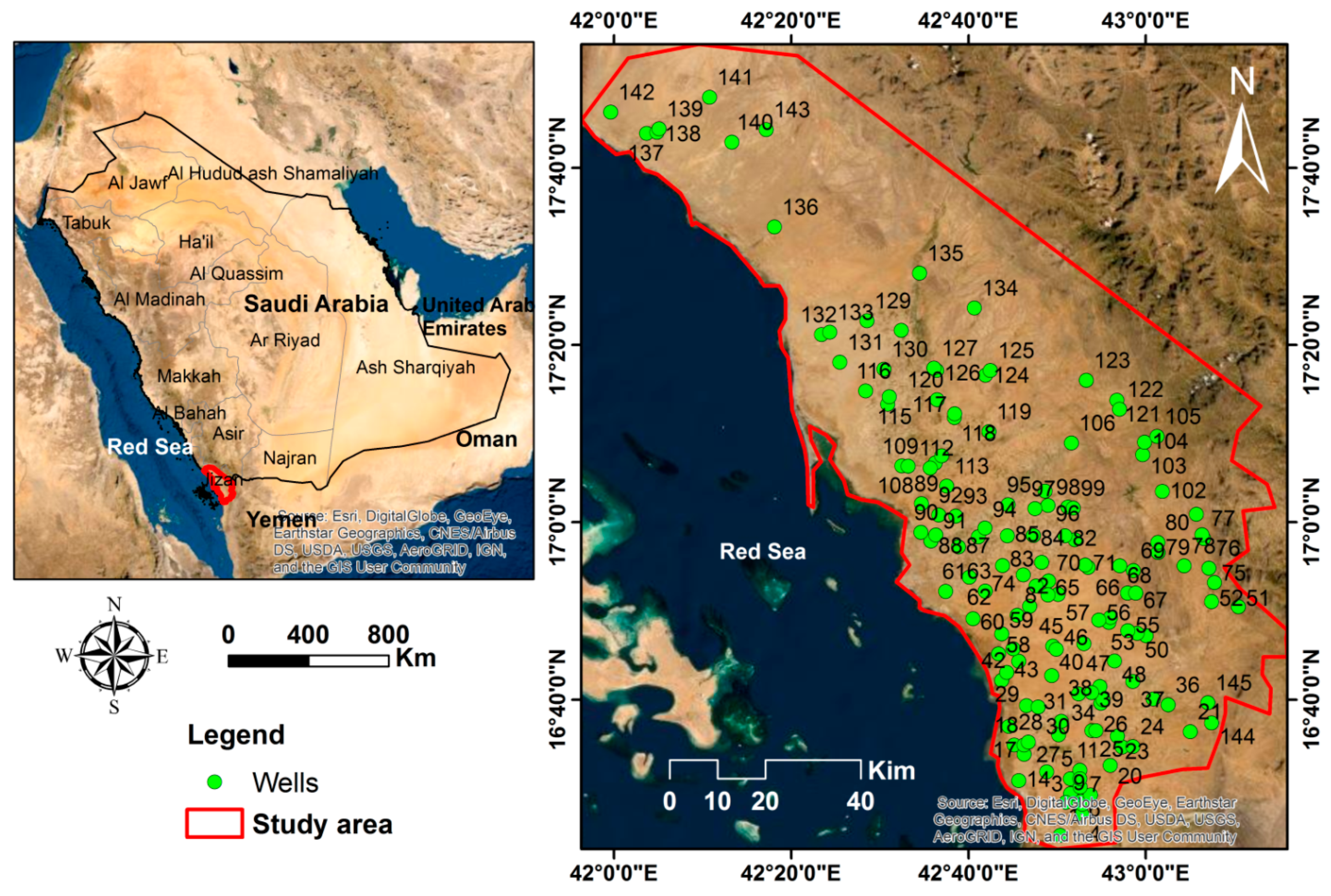
Figure 1. Location of the study area and wells.
Water 15 02448 g001
Figure 2. Average temperatures, precipitation, and relative humidity in the study area (Station Jizan, 2021).
Water 15 02448 g002
Figure 3. The description of the ANN model for modelling the WAWQI.
Water 15 02448 g003
Figure 4. The typical architecture of SVM (one-dimensional linear). ε is the tolerance margin, ξ and ξ* are the control or slack variables of the error from the regression function, points on margins are called support vectors (figure adapted after Cantillo-Luna et al. [51]).
Water 15 02448 g004
Figure 5. (a) Groundwater level (m.asl), (b) depth to groundwater in the study area.
Water 15 02448 g005
Figure 6. Total dissolved solids (TDS) zonation map for the study area.
Water 15 02448 g006
Figure 7. K+ (a) Na+ (b) Ca2+ (c) Mg2+ (d) distribution (zonation map) for the study area.
Water 15 02448 g007aWater 15 02448 g007b
Figure 8. SO42– (a) Cl (b) HCO3 (c) NO3 (d) distribution (zonation map) for the study area.
Water 15 02448 g008aWater 15 02448 g008b
Figure 9. Classification of water quality according to the WAWQI.
Water 15 02448 g009
Figure 10. WAWQIs spatial distribution in the study area.
Water 15 02448 g010
Figure 11. Observed and predicted WAWQI values.
Water 15 02448 g011
Figure 12. ANN modelling validation with a best performance MSE of 0.048016 at iteration 13.
Water 15 02448 g012
Figure 13. Predicted vs. calculated WAWQI for the applied models in the training stage (right) and testing stage (left).
Water 15 02448 g013aWater 15 02448 g013b
Table 1. Descriptive statistics for physicochemical variables and WHO standards for drinking water.
ElementMin.Max.AverageStandard DeviationWHO Guidelines [44]
pH6.38.77.70.37
TDS (mg/L)128.08320.01709.61293.01000
TH (mg/L)90.63676.6640.8526.7500
Ca2+ (mg/L)23.5831.7157.7131.6200
Mg2+ (mg/L)4.4388.860.055.930
Na+ (mg/L)1.61291.4307.6276.3200
K+ (mg/L)1.2188.512.427.612
Cl (mg/L)12.83669.1571.6602.3250
HCO3 (mg/L)9.2518.1217.589.4350
SO42− (mg/L)7.21098.5319.8221.9350
NO3 (mg/L)0.0034.11.84.450
Table 2. Physicochemical parameters’ weights and relative weights [33].
ParametersWeight (wi)Relative Weight (Wi)
pH40.100
TDS50.125
TH30.075
Ca2+30.075
Mg2+30.075
Na+40.100
K+20.050
Cl50.125
HCO310.025
SO42−50.125
NO350.125
Table 3. Classification of water quality according to the WQI type and range [45].
WAWQIWater Type
<50Excellent
50–100Good
100.1–200Poor
200.1–300Very poor
>300.1Unsuitable
Table 4. Descriptive statistics for all input and output variables.
VariableMeanSE MeanStDevMinimumQ1MedianQ3Maximum
pH7.660.030.316.337.487.677.828.68
TDS17101081298128803140821288320
TH640.843.9528.590.6303.4473.2864.03676.6
Ca2+157.711.0132.023.473.5116.6193.0831.7
Mg2+60.024.6656.084.3727.0339.0083.11388.80
Na+307.623.0277.31.6116.4242.1365.11291.3
K+12.442.3027.681.173.525.477.62188.46
Cl571.650.2604.412.8173.4427.9691.63669.1
HCO3217.457.4589.699.15151.94206.25266.05518.06
SO42–319.818.5222.77.2141.2287.2427.51098.4
NO31.8370.3634.3740.0000.3300.8001.46534.140
WAWQI125.417.2687.4020.3064.6199.46161.33592.31
SE Mean: standard error of mean, St Dev: standard deviation, Q1: first quartile, Median: middle number, Q3: third quartile.
Table 5. The Pearson correlation coefficient of the variables, values of R > 0.5, are shown in bold.
pHTDSTHCa2+Mg2+Na+K+ClHCO3SO42–NO3
pH1
TDS−0.0981
TH−0.2030.8731
Ca2+−0.1980.8370.9611
Mg2+−0.1820.8030.9180.7711
Na+0.0140.9060.5860.5670.5331
K+−0.004−0.0450.003−0.0040.012−0.1081
Cl−0.0530.9770.8470.8180.7700.891−0.0561
HCO3−0.2200.0070.0210.0110.033−0.0040.045−0.1021
SO42–−0.1400.7530.6750.6290.6480.6680.0080.6100.0911
NO3−0.2730.1520.2610.2890.1850.0300.0090.0910.2350.2531
Table 6. Model coefficients from multiple regressions.
EstimateSEp Value
Intercept −0.0057310.00707810.41958
pH1.42920.0008888<0.00000
TDS0.0124811.18 × 10−5<0.00000
TH0.0695230.0186680.0002884
Ca2+−0.0986390.0466130.036195
Mg2+0.0256490.0768170.73898
Na+0.0500021.91 × 10−5<0.00000
K+0.416671.09 × 10−50
Cl0.0500321.73 × 10−5<0.00000
HCO30.0071651.02 × 10−5<0.00000
SO42–0.035741.30 × 10−5<0.00000
NO30.249986.28 × 10−50
Table 7. The performance indices of the developed models for the WAWQI during the training and testing stages.
Model/IndicesMEMAERMSEMAPE %RR2
Fit binary treeTraining0.006.06610.0854.9200.98840.9942
Testing0.007.72310.2228.7720.97010.9849
SVM (linear)Training1.9203.3883.8253.3800.99880.9994
Testing3.1854.4694.6885.6420.99760.9988
SVM (polynomial kernel)Training−0.2346.4248.1445.4530.99530.9976
Testing−1.0788.30210.0409.3430.97530.9876
Gaussian process regression (GPR)Training0.000.19350.25520.2341.001.00
Testing0.000.25290.3260.3911.001.00
Linear regression (stepwise)Training0.000.00230.00280.00251.001.00
Testing0.000.00240.00290.00141.001.00
ANNTraining0.0880.0880.08840.09691.001.00
Testing0.0740.0740.0750.09821.001.00
Table 8. The best subset regression analysis for determining the best input combinations to model WQI.
No. of VariablesVariablesMSER2Adjusted R2Akaike’s AICSchwarz’s SBCAmemiya’s PC
1NO37467.340.020.0231295.1391301.0920.984
2SO4/NO33356.680.560.5611180.1811189.1120.445
3HCO3/SO4/NO33342.150.570.5631180.5271192.4340.446
4Cl/HCO3/SO4/NO3197.3590.9750.974771.240786.1240.027
5K/Cl/HCO3/SO4/NO360.9570.9920.992601.848619.7080.008
6Na/K/Cl/HCO3/SO4/NO317.2200.9980.998419.503440.3400.002
7Mg/Na/K/Cl/HCO3/SO4/NO31.7731.0001.00090.825114.6390.000
8Ca/Mg/Na/K/Cl/HCO3/SO4/NO30.1841.0001.000−236.474−209.6840.000
9TH/Ca/Na/K/Cl/HCO3/SO4/NO30.1841.0001.000−236.474−209.6840.000
10TDS/TH/Ca/Na/K/Cl/HCO3/SO4/NO30.1611.0001.000−255.097−225.3300.000
11pH/TDS/TH/Ca/Na/K/Cl/HCO3/SO4/NO30.0001.0001.0000.0000.0000.000
The best models for the selection criteria are displayed in bold.
Disclaimer/Publisher’s Note: The statements, opinions and data contained in all publications are solely those of the individual author(s) and contributor(s) and not of MDPI and/or the editor(s). MDPI and/or the editor(s) disclaim responsibility for any injury to people or property resulting from any ideas, methods, instructions or products referred to in the content.