Article

Utility of Open-Access Long-Term Precipitation Data Products for Correcting Climate Model Projection in South China

1
China Institute of Water Resources and Hydropower Research, Beijing 100038, China
2
Research Center on Flood & Drought Disaster Reduction of the Ministry of Water Resources, Beijing 100038, China
3
Guangdong Engineering Technology Research Center of Smart and Ecological River, Shenzhen 518020, China
4
School of Civil Engineering and Transportation, South China University of Technology, Guangzhou 510641, China
*
Author to whom correspondence should be addressed.
Water 2023, 15(16), 2906; https://doi.org/10.3390/w15162906
Submission received: 4 July 2023 / Revised: 6 August 2023 / Accepted: 9 August 2023 / Published: 11 August 2023

Abstract

:
Insufficient precipitation observations hinder the bias-correction of Global Climate Model (GCM) precipitation outputs in ungauged and remote areas. As a result, the reliability of future precipitation and water resource projections is restricted for these areas. Open-access quantitative precipitation estimation (QPE) products offer a potential solution to this challenge. This study assesses the effectiveness of three widely used, long-term QPEs, including ERA5, PERSIANN-CDR, and CHIRPS, in bias-correcting precipitation outputs from the CMIP6 GCMs. The evaluation involves the reproduction of precipitation distribution, streamflow simulation utility based on a hydrological model, and the accuracy of extreme indices associated with rainstorm/flood/drought events. This study selects the Beijiang basin located in the subtropical monsoon area of South China as the case study area. The results demonstrate that bias-correction using QPEs improves the performance of GCM precipitation outputs in reproducing precipitation/streamflow distribution and extreme indices, with a few exceptions. PCDR generally exhibits the most effective bias-correction utility, consistently delivering reasonable performance across various cases, making it a suitable alternative to gauge data for bias-correction in ungauged areas. However, GCM outputs corrected by ERA5 tend to overestimate overall precipitation and streamflow (by up to about 25% to 30%), while the correction results of CHIRPS significantly overestimate certain extreme indices (by up to about 50% to 100%). Based on the revealed performance of QPEs in correcting GCM outputs, this study provides references for selecting QPEs in GCM-based water resource projections in remote and ungauged areas.

1. Introduction

Reliable projection of future precipitation and water resource change is important for sustainable agricultural, ecological, and social economic development under global warming and climate change [1,2,3,4,5]. The climate projections from the Global Climate Models (GCMs) are regarded as one of the most reasonable tools to project the precipitation and hydrological change under the future climate change scenarios [3,6]. The Coupled Model Intercomparison Project (CMIP) proposed by the World Climate Research Programme (WRCP) integrated a large number of GCMs developed from various research institutes worldwide [7,8,9]. The GCMs of the CMIP have provided useful climate projection data supporting many research studies of future precipitation and water resource change, including flood and drought disaster [10,11,12,13], water body and ecosystem change [14,15], and hydropower potential [6,16,17], largely enhancing the knowledge about mitigation policy making concerning climate change for the water resource sectors. In recent years, the latest CMIP phase 6 (CMIP6) has been conducted, which integrates and provides an unprecedented number of GCMs with significantly improved resolution and simulation performance [7,18,19], showing a brighter prospect for the research and applications of water resource projection and planning.
Nevertheless, due to the inadequacies in the model mechanism and structure as well as the initial state of the GCMs, the climate projection outputs from GCMs often exhibit coarse spatial resolution, high uncertainty, and systematic bias compared to reality [20,21,22]. Although regional climate models (RCMs) as an effective tool have been widely applied to downscale the spatial resolution of GCMs [23,24], some studies reported that systematic bias might exist in the RCM outputs and needs correction [25,26,27]. Since precipitation plays a crucial role in water resource applications, the bias in the precipitation projection might be aggravated in hydrological modeling and extreme event reproduction. Therefore, reliable bias-correction on the GCM outputs is typically necessary before the formal applications [19,20,21]. Statistical bias correction approaches are widely used because they offer satisfactory bias correction efficiency at a low computational cost. These approaches typically employ historical gauge observations as references and establish regression relationships with GCM historical outputs [28,29]. However, the application of statistical bias correction approaches is often limited in remote and ungauged areas due to insufficient historical climate observations, particularly for precipitation, which exhibits high heterogeneity and is challenging to be estimated through spatial interpolation [5,30,31].
In recent years, several open-access quantitative precipitation estimation (QPE) products based on satellite remote sensing or reanalysis approaches have been developed. These products aim to provide alternative precipitation data for remote and ungauged areas. Notable QPEs include the Tropical Rainfall Measurement Mission (TRMM) [32], the Climate Prediction Center (CPC) Morphing technique (CMORPH) [33], and the Integrated Multi-satellite Retrievals for Global Precipitation Measurement (IMERG) [34]. These QPEs typically offer wide spatial coverage and high spatiotemporal resolution, fulfilling the data requirements for ungauged areas.
Nevertheless, most current QPEs have relatively short data records that begin in the 2000s, which limits their overlapping period with the historical outputs of GCMs (which end in 2014 for CMIP6) [35]. Consequently, the application of these QPEs for bias-correction of GCM outputs is restricted. To address this issue, several long-term QPEs have been proposed, such as the ERA5 precipitation product [36], the Precipitation Estimation from Remotely Sensed Information using Artificial Neural Networks–Climate Data Record (PERSIANN-CDR) [37,38], and the Climate Hazards Group (CHG) InfraRed Precipitation with Station (CHIRPS) [39]. These long-term QPEs not only have long data records starting from the 1940s to 1980s but also have an adequate overlapping period with GCM historical outputs. Furthermore, they have been validated for their accuracy and performance in conventional hydrological practices [30,40,41], indicating great potential for bias-correction of GCM outputs and other climatic applications.
Some studies have been conducted on the climatic utility of long-term QPEs like GCM output bias-correction. Zhu et al. [28] evaluated the performance of PERSIANN-CDR in bias-correcting 16 GCM outputs from CMIP5 in South China and found that most of the GCMs showed improvement after bias-correction using this QPE. Katiraie-Boroujerdy et al. [29] employed PERSIANN-CDR to correct precipitation outputs from seven CMIP5 GCMs in Iran and assessed the accuracy of the corrected outputs in calculating extreme indices. Babaousmail et al. [42] used CHIRPS to correct precipitation outputs from five CMIP6 GCMs for future precipitation projections over the Mediterranean and Sahara. These studies have contributed to our understanding and confidence in performing reliable precipitation projections for ungauged areas using corrected GCM outputs. However, there are fewer studies that evaluate and compare the abilities of multiple open-access QPEs for bias-correction of GCM precipitation outputs, particularly for the state-of-the-art CMIP6 GCMs.
The research purpose of this study is to evaluate and compare the performance of multiple widely-used, open-access, long-term QPEs in bias-correcting GCM precipitation outputs. Such QPEs include ERA5, PERSIANN-CDR, and CHIRPS. Specifically, this study will focus on improvements of bias-correction in the distribution of precipitation, the utility of hydrological modeling, and the ability to reproduce extreme precipitation and hydrological events of the bias-corrected GCM precipitation outputs. The Beijiang basin, situated in the subtropical monsoon humid region of South China (Figure 1), which experiences frequent flood and drought disasters, was chosen as the case study area. Additionally, four CMIP6 GCMs developed by various institutes worldwide were selected as the cases for analysis, and the GR4J hydrological model was employed to generate the streamflow outputs by the GCM precipitation outputs. Different to the former studies that focused on only a single QPE, this study evaluated and inter-compared the climatic utility of multiple QPEs, revealing their performance differences in GCM correction for different aspects. The findings of this study are expected to provide valuable insights into the selection and application of multiple QPEs for GCM-based water resource projection in remote and ungauged areas.

2. Materials

2.1. Study Area

The Beijiang basin, located in the southeast monsoon humid region of South China in East Asia (Figure 1), was selected as the case study area. The Beijiang River, a major tributary of the Pearl River, has an annual mean streamflow of about 3.4 × 10 10   m 3 , covering a drainage area of 34,039 km2 over the Hengshi hydrological station. The local climate of the Beijiang basin is characterized as a subtropical monsoon humid climate that belongs to the subtropical humid type (Cf) according to the Trewartha climate classification, with an average annual precipitation of over 1700 mm and an annual mean air temperature of 25 °C from 1985 to 2014. The intra-annual distribution of precipitation is highly uneven, with more than 70% occurring during the wet season. As a result, flood and drought disasters frequently occur in the Beijiang basin [40], posing a threat to the downstream Pearl River Delta, which is a densely populated and highly developed area, and resulting in significant economic losses. Therefore, the Beijiang basin serves as a suitable case study for illustrating the climatic utility of QPEs in correcting GCM precipitation outputs, particularly regarding the reproduction of extreme events of the bias-correction results.

2.2. Long-Term Quantitative Precipitation Estimation (QPE) Products

2.2.1. ERA5 Reanalysis

ERA5 (the fifth generation of European Centre for Medium-Range Weather Forecasts (ECMWF) Reanalysis) [36] is the latest open-access global atmospheric reanalysis data developed and maintained by the ECMWF. ERA5 is produced by the latest Integrated Forecasting System (IFS Cycle 41r2) using an advanced four-dimensional variational assimilation algorithm and integrates various observation sources like satellite remote sensing, meteorological stations, and ground-based weather radars. ERA5 provides long-term global atmospheric reanalysis data including precipitation from 1940 to the present, with a high spatial resolution of 0.25° and an hourly temporal resolution. The ERA5 precipitation data is open-access on the website of the Copernicus Climate Change Service (https://doi.org/10.24381/cds.f17050d7, accessed on 6 August 2023). This study used the daily ERA5 precipitation data for the period of 1984 to 2014.

2.2.2. PERSIANN-CDR (PCDR)

The Precipitation Estimation from Remotely Sensed Information using Artificial Neural Networks–Climate Data Record (PERSIANN-CDR, hereafter referred to as PCDR) [38] is an open-access long-term gridded precipitation product developed by the Center of Hydrology and Remote Sensing (CHRS) at the University of California, Irvine. The PCDR is produced by an artificial neural network that establishes regression relationships between the satellite infrared data and ground-based precipitation datasets like the Stage-IV radar data, using the GridSat-B1 long-term satellite infrared data as input; then, the Global Precipitation Climatology Project (GPCP) coarse-resolution precipitation data (2.5°) are used to correct the output precipitation data to obtain the final products. Consequently, the PCDR precipitation product has a long data record spanning from 1983 to the present, covering the latitude band of 60° N–60° S, with the spatial resolution of 0.25° and a daily timescale. The PCDR data is open-access on the CHRS data portal (https://chrsdata.eng.uci.edu/, accessed on 6 August 2023). This study used the daily PCDR data for the period of 1984–2014.

2.2.3. CHIRPS

The Climate Hazards Group (CHG) Infrared Precipitation with Station (CHIRPS) [39] is an open-access, long-term, high-resolution precipitation product based on thermal infrared satellite remote sensing, which is developed by the CHG at the University of California, Santa Barbara. The CHIRPS is designed mainly for the purpose of climate hazard monitoring in ungauged areas.
In the production process performed by CHG, the CHIRPS is generated based on two long-term, high-resolution thermal infrared datasets named the GridSat and the Climate Prediction Center Thermal Infrared (CPC TIR), using the statistical regression relationships between the thermal infrared data and other precipitation products like Tropical Rainfall Measurement Mission (TRMM). Subsequently, the preliminary precipitation data undergo climatological correction by the CHPclim global precipitation climatology and further correction by the global ground-based gauge precipitation observation data, thus generating the final CHIRPS product. The CHIRPS provides long-term, quasi-global daily precipitation data since 1981, with spatial coverage between the latitude band of 50° S–50° N and a high spatial resolution of 0.05°. The CHIRPS data are open-access on the CHG website (https://data.chc.ucsb.edu/products/CHIRPS-2.0/, accessed on 6 August 2023). This study used the daily CHIRPS data for the period of 1984–2014.

2.3. CMIP6 Projection Outputs

The Coupled Model Intercomparison Project phase 6 (CMIP6) is the latest iteration of the CMIP conducted by the WRCP [7,18]. It represents a collaborative international endeavor aimed at advancing people’s understanding of climate dynamics and projections. CMIP6 incorporates a diverse array of GCMs from various institutions worldwide. Compared to its predecessor, CMIP5, the GCMs utilized in CMIP6 have made significant improvements in terms of coupling of geophysical process, spatiotemporal resolution, and simulation accuracy of the global climate [7].
This study utilized the GCM historical outputs from four GCMs in the CMIP6 historical experiment as the cases to evaluate the bias-correction utility of the QPEs. The selected GCMs are CanESM5 [43], INM-CM4-8 [44], IPSL-CM6A-LR [35], and MIROC6 [45] (Table 1). These GCMs were selected according to the data availability of necessary meteorological variables like precipitation and air temperature. The historical period for CMIP6 ranges from 1850 to 2014. To align with the available records of QPEs and ground observations, the GCM precipitation outputs, as well as mean/maximum/minimum air temperature outputs from these four GCMs, were obtained for the period spanning 1985 to 2014, at a daily timescale. Prior to bias-correction, the GCM outputs were converted to a basin-averaged scale using the Thiessen polygon weighted averaging approach. The CMIP6 GCM output data were obtained from the Earth System Grid Federation (ESGF) website (https://esgf-node.llnl.gov/, accessed on 6 August 2023).

2.4. Ground-Based Observation Data

Daily gauge precipitation, as well as daily mean/maximum/minimum air temperature data spanning from 1984 to 2014, were obtained from 30 meteorological stations located over the Beijiang basin (Figure 1) in South China. The gauge precipitation data served as a reference for assessing the performance of the QPEs and the bias-corrected GCM precipitation outputs. It was also used as input for calibrating the GR4J hydrological model. The air temperature data were utilized to calculate the potential evapotranspiration, which is a necessary input for the GR4J model. To ensure consistency, all meteorological data at the station scale were transformed into a basin-averaged scale using the Thiessen-polygon-based weighted averaging approach.
Additionally, ground-based daily streamflow observations from the Hengshi Station spanning from 1985 to 2011 were obtained. These observations served as a benchmark for calibrating the GR4J model and evaluating the simulated streamflow generated by the bias-corrected GCM precipitation outputs.

3. Methods

3.1. Quantile Mapping (QM) Statistical Bias-Correction Approach

The empirical quantile mapping (QM) statistical bias-correction approach was employed to correct the raw GCM precipitation and air temperature outputs in this study. The QM approach is widely recognized as one of the most effective methods for bias-correction, offering advantages such as satisfactory performance, low implementation cost, and low computational requirements when applied to bias-correction [25,27,28,46]. The QM approach typically relies on the availability of observed precipitation data to serve as reference data for bias-correction, alongside historical GCM outputs to establish empirical regression relationships. Considering that geophysical variables often exhibit different distributions across calendar months, the bias-correction process was carried out separately for each calendar month.
The reference data, the corresponding GCM historical outputs, and the GCM outputs that require bias-correction for calendar month m are denoted as X R , m , X H , m , and X G , m , respectively. Their empirical cumulated distribution functions (CDFs) are calculated as:
p X r = r n + 1
where X r is the data record from X R , m , X H , m , or X G , m ; p is the empirical CDF; r is the rank of the value of record X r among all data records; and n is the number of records. The calculated empirical CDFs of X R , m , X H , m , and X G , m are denoted as p R , m , p H , m , and p G , m , respectively, and their reverse functions are denoted as F R , m , F H , m , and F G , m , respectively.
For precipitation, the form of the QM approach can be expressed as:
X G , m = X G , m F R , m p / F H , m p
where X G , m and X G , m are the GCM precipitation output records before and after bias-correction, m determines the calendar month of the GCM output record, and p is the frequency corresponding to X G , m , i.e., p = p G , m ( X G , m ) . Conversely, for air temperature, the form of the QM approach can be expressed as:
X G , m = X G , m + F R , m p X F H , m p X
where X G , m and X G , m denote the GCM air temperature outputs before and after bias-correction.
In this study, bias-correction and evaluation of GCM precipitation outputs were conducted for the 30-year period from 1985 to 2014. The air temperature outputs of the GCMs were also derived and bias-corrected to calculate the potential evapotranspiration data, which served as the input for the GR4J model. Considering that relative studies of GCM output correction used a record length of about 20 years for constructing bias-correction models [28,42], as well as to provide adequate record length for validating bias-correction results of GCM outputs, this study used 20 years for establishing the QM approach, while the residual 10 years were used to validating the bias-correction results. The GCM precipitation outputs, along with the QPE data as the bias-correction reference, were temporally divided into two parts: a 20-year “training set” used to establish the empirical statistical relationship for the QM approach (i.e., F R , m and F H , m in Equation (2)) and a 10-year “validation set” used to evaluate the bias-correction performance. The evaluation was performed solely on the “validation set”.
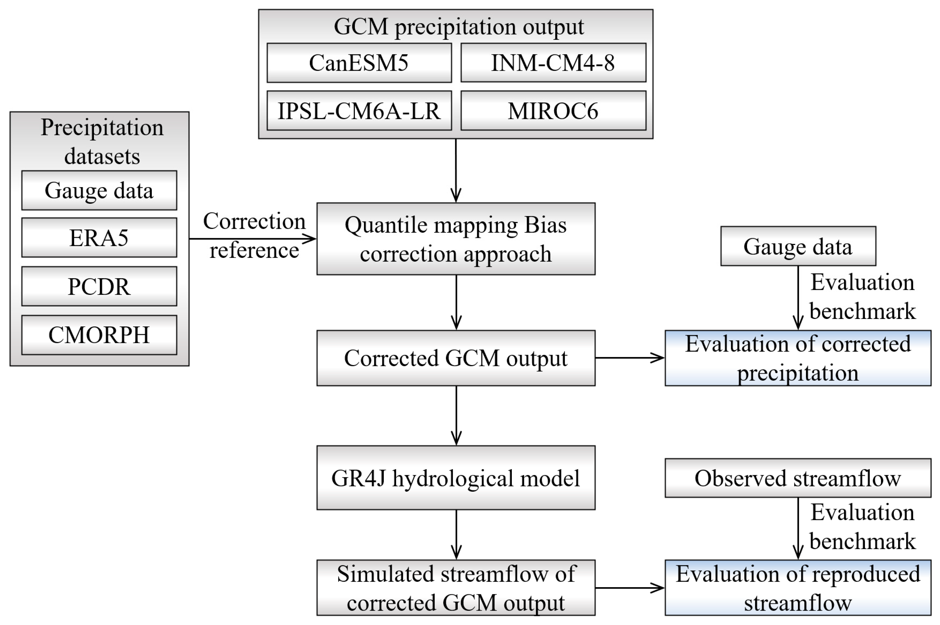
To mitigate the potential impact of temporal partitioning on the bias-correction evaluation, we implemented a cross-validation-like procedure. Instead of simply dividing the GCM precipitation outputs and QPE data into consecutive front and rear parts, we randomly sampled 10 years from the 30-year period of 1985–2014 to create the “validation set”, while the remaining 20 years were designated as the “training set”. This random sampling was repeated 100 times, resulting in 100 sample sets. Subsequently, bias correction and evaluation were performed for each of the 100 sample sets individually. For each of the four GCMs, the precipitation outputs were bias-corrected using three different QPEs, along with the gauge data, enabling the assessment and comparison of the utility of QPEs for bias-correction. The flowchart depicting the evaluation procedure in this study is presented in Figure 2.

3.2. Assessment Metrics

Multiple assessment metrics were employed to evaluate the accuracy of the QPE data and the simulated streamflow generated by the hydrological model. These metrics include the Pearson correlation coefficient (R), the root mean square error (RMSE), the relative bias (RB), the Kling–Gupta efficiency coefficient (KGE) [47], and the Nash–Sutcliffe efficiency coefficient (NSE). The calculations for these metrics are as follows:
R = S S ¯ O O ¯ S S ¯ O O ¯
R M S E = S O n
R B = S ¯ O ¯ 1 × 100 %
N S E = 1 S O 2 O O ¯ 2
K G E = 1 r 1 2 + α 1 2 + β 1 2
where
r = R α = σ S σ O β = S ¯ O ¯
where S and O are the data needing evaluation and the benchmark data, respectively; S ¯ and O ¯ are their mean values, while σ S and σ O are their standard deviations respectively; n is the number of records. The R assesses the linear correlation between estimations and benchmarks. The RMSE measures the deviation between estimations and benchmarks. The RB quantifies the overall systematic bias of estimations. The NSE and KGE evaluate the consistency between the estimation series and the benchmarks, particularly in the context of evaluating the simulated streamflow.
In line with previous CMIPs, the CMIP6 historical experiment aims to reproduce historical climate characteristics and signals under natural and anthropogenic forcings, rather than capturing the exact temporal variation of climate variables in reality. Therefore, the evaluations of bias-correction for CMIP6 GCM outputs in this study primarily focus on the reproduction of the statistical distribution of historical precipitation/streamflow and the ability capturing extreme events. To assess whether the GCM outputs have the same distribution as observations in reality, the D m a x metric of the two-sample Kolmogorov–Smirnov test (K-S test) [48] is employed. The K-S test, as a nonparametric test, measures the maximum distance ( D m a x ) between the empirical cumulative distribution function (CDF) curves of the two samples along the frequency axis, in order to quantify the deviation between the two samples’ distribution. A smaller D m a x value indicates better consistency between the distributions of the two samples.
A total of 11 extreme indices were utilized as cases to evaluate and compare the capability of the GCM precipitation outputs and their simulated streamflow in reproducing extreme events. These indices are listed in Table 2. Among them, 5 precipitation-related extreme indices were selected from the recommended list of the Climdex project from the Australian Research Council (ARC) Centre of Excellence for Climate Extremes (https://www.climdex.org/learn/indices/, accessed on 6 August 2023). Additionally, 6 hydrology-related extreme indices were established based on widely used indicators in hydrological applications like water resource management and flood/drought prevention. The 11 extreme indices encompass indicators for total water resources, rainstorm/flood events, and drought disasters. All the extreme indices are annual scale indices; hence, they were calculated for each year of the 10 years of the “validation set” for the GCM outputs, respectively, and the median and extreme values over the 10 years were used for validation (for details, please see the Section 4).

3.3. GR4J Hydrological Model

The GR4J (Génie Rural à 4 paramètres Journalier) hydrological model [49] was employed to simulate streamflow using the bias-corrected GCM precipitation output, enabling the assessment of the QPE-based bias-corrected GCM outputs in streamflow simulation. The GR4J model is a conceptual lumped hydrological model characterized by its simple structure, requiring only precipitation and potential evapotranspiration as input variables. Despite its simplicity, the model is capable of effectively simulating daily streamflow and has been widely applied in various regions worldwide, including the Beijiang basin employed by this study [50]. Prior to application, the GR4J model necessitates calibration, which involves determining the values of four parameters: the maximum capacity of the production storage X 1 , the groundwater exchange coefficient X 2 , the maximum capacity of the routing storage X 3 , and the unit hydrograph time base coefficient X 4 .
In this study, the calibration of the GR4J model was carried out using the Shuffled Complex Evolution–University of Arizona (SCE-UA) algorithm [51], with the KGE based on streamflow observations serving as the objective function. The calibration period spanned from 1985 to 2000, while the validation period covered 2001 to 2011. It is worth noting that the GR4J model typically requires a “warm-up” period of at least one year in streamflow modeling. For this study, the year 1984 was designated as the “warm-up” period.
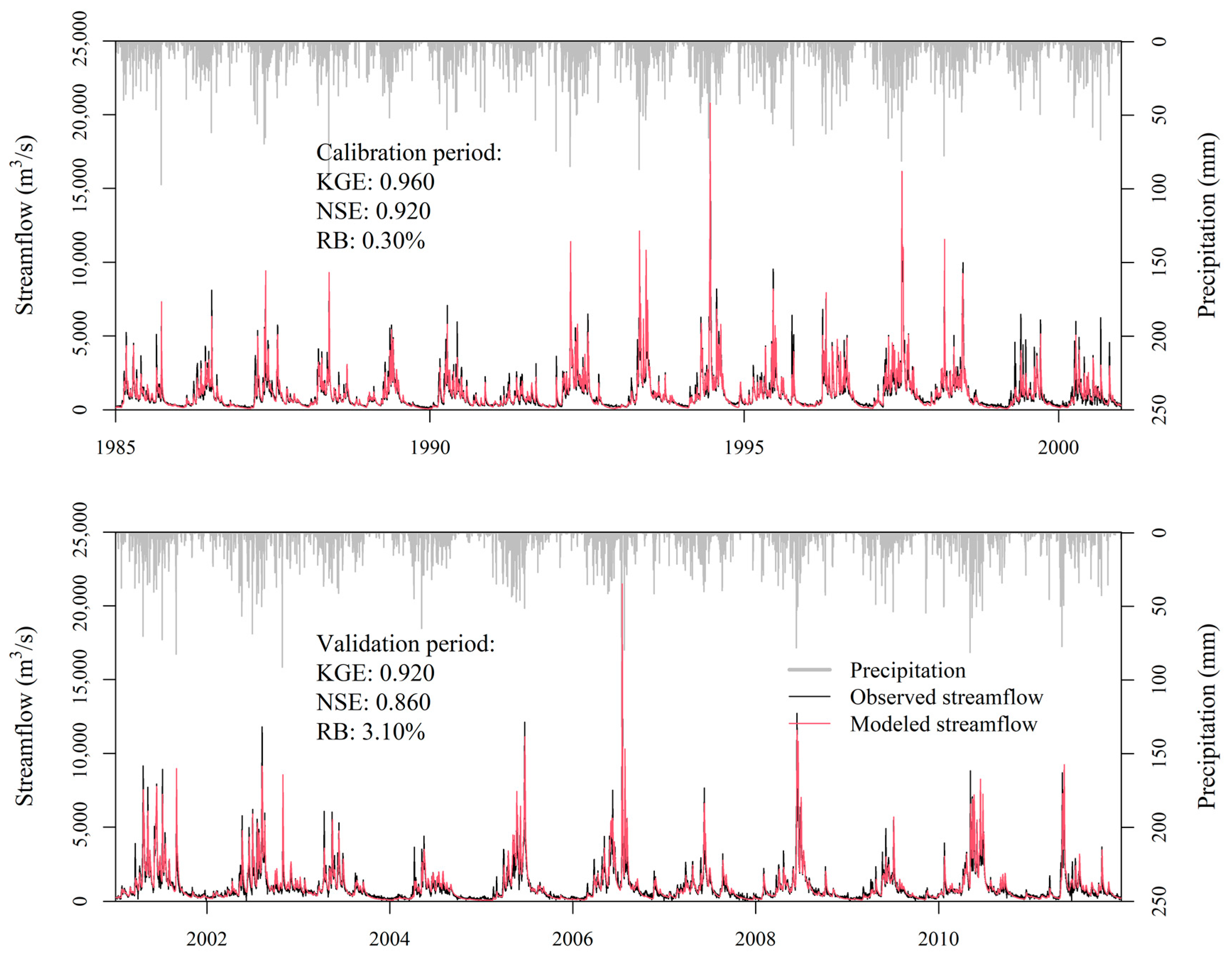
The calibration and validation results of the GR4J model are depicted in Figure A1 in Appendix A. The KGEs and NSEs for both periods surpass 0.9 and 0.85, respectively, while the RBs approach zero. These findings indicate the satisfactory applicability of the GR4J model for the Beijiang basin and its suitability for evaluating the hydrological performance of bias-corrected GCM precipitation outputs.
To evaluate the performance of the calibrated GR4J model in modeling peak flow and low flow, the extreme indices related to flood and drought, i.e., Qx1d, Qx5d, and Qn7d, were calculated for each year from 1985 to 2011, and their medians and high/low values during the period are shown in Table A1 in Appendix A. The results show that the Qx1d and Qx5d modeled by the GR4J model were close to observations, for both median and high values, revealing the acceptable ability of the calibrated GR4J model in modeling flood peaks; nevertheless, the median and low values of Qn7d by the GR4J model show underestimation to observation.

4. Results

4.1. Evaluation of the QPEs

To properly evaluate the bias-correction utility of the QPEs, it is crucial to first assess their characteristics and accuracy. The QPE precipitation data and their simulated streamflow were assessed with reference to gauge data and streamflow observations, respectively. The assessment metrics are presented in Table 3 for QPE precipitation data and Table 4 for the corresponding simulated streamflow.
The results indicate that, at the daily timescale, ERA5 exhibits the highest R with gauge data, surpassing 0.8, and the smallest root mean square error (RMSE) of 5.4 mm. Meanwhile, PCDR and CHIRPS demonstrate lower accuracy, with an R of approximately 0.7 and RMSEs of about 7 mm. However, it is worth noting that ERA5 shows a noticeable overestimation of around 17% of total precipitation, while the RBs of PCDR and CHIRPS are considerably smaller. At the monthly timescale, all QPEs exhibit high correlation coefficients (Rs) exceeding 0.9. Among them, CHIRPS demonstrates the best performance, presenting the highest R and the smallest RMSE.
Regarding streamflow simulation, it can be observed that the systematic bias in ERA5 propagated into the simulated streamflow. During the period of 1985–2000, ERA5-simulated streamflow demonstrates low KGEs and NSEs below 0.5, along with a significantly higher RB exceeding 40%. However, for the period of 2001 to 2011, the RB of ERA5-simulated streamflow decreases, likely due to the reduced bias in ERA5 precipitation during this period. In contrast, the results obtained from PCDR and CHIRPS exhibit consistent performance for both periods, showing acceptable KGEs and Rs around 0.8, as well as NSEs ranging from 0.6 to 0.7. Overall, both PCDR and CHIRPS demonstrate satisfactory accuracy in terms of precipitation and exhibit good performance in streamflow simulation. On the other hand, ERA5’s apparent overestimation of precipitation leads to poor performance in streamflow modeling
Table 5 and Table 6 present the median and 90%/10% percentile values of extreme indices derived from QPEs during the period of 1985 to 2014 for precipitation and simulated streamflow, respectively. It is important to note that only extreme indices related to disasters, such as Rx1d and Qx1d, are included in the tables. The 90% percentile values (90% of data records below or equal to this value) are displayed for most extreme indices, as they indicate flood disasters, while the 10% percentile values (only 10% of data records below this value) are provided for Qn7d, as it represents drought disasters. The results reveal that for rainstorm-related extreme indices (Rx1d, Rx5d, and R50mm), all QPEs exhibit similar magnitudes to the gauge data or streamflow observations. Although CHIRPS tends to overestimate Rx1d and R50mm, the over- or underestimations observed in the QPEs are generally within acceptable ranges. However, for flood-related extreme indices (Qx1d and Qx5d), ERA5 shows a noticeable overestimation in the median values, while CHIRPS demonstrates an apparent overestimation in the high values of Qx1d. In terms of drought-related extreme indices (CDD and Qn7d), all QPEs consistently underestimate these indices. In summary, both ERA5 and CHIRPS exhibit overestimation in extreme events related to rainstorms and floods, whereas PCDR accurately reproduces extreme indices in most cases.

4.2. Evaluation of GCM Precipitation Outputs Bias-Corrected by QPEs

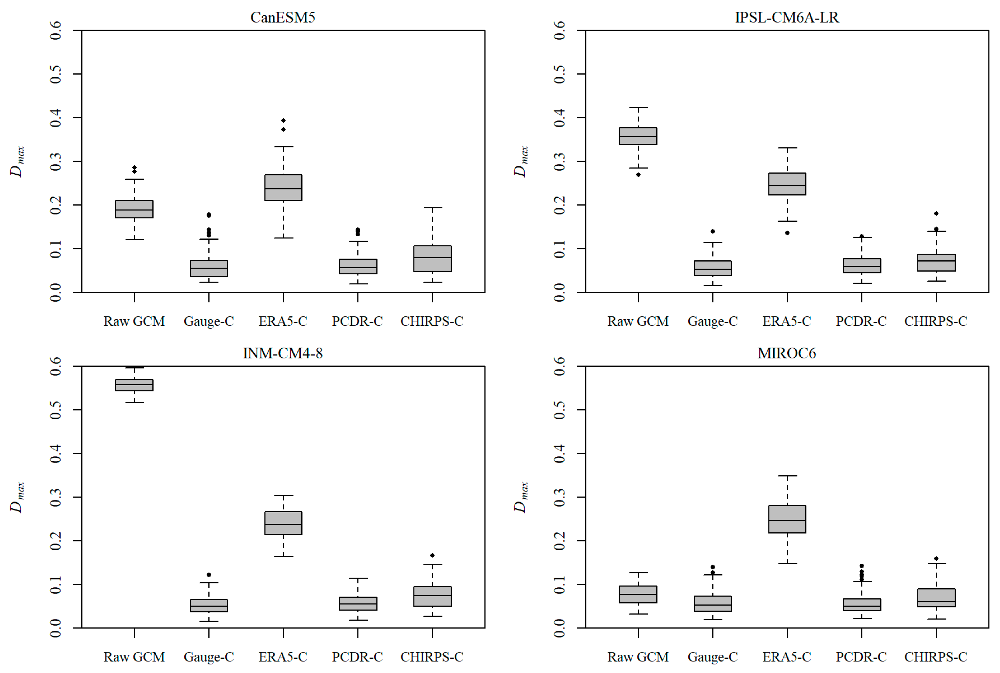
Figure 3 shows D m a x values of the raw and bias-corrected GCM precipitation outputs. The boxplots in the figure represent the distribution of D m a x values among the results of 100 sample sets. The results show that, for the raw GCM outputs, MIROC6 exhibits the best fitness in terms of the distribution of daily precipitation, with generally low D m a x values below 0.1. Nevertheless, the remaining GCM outputs yield much higher D m a x values, in which INM-CM4-8 shows the highest value, close to 0.6. This highlights the need for bias-correction for most GCMs.
Regarding the bias-corrected GCM outputs using QPEs, the results show that PCDR achieves the best performance in improving the distribution of precipitation among the three QPEs, with D m a x values close to those bias-corrected by gauge data. Conversely, the bias-correction results of ERA5 exhibit the poorest performance, with high D m a x values for the corrected GCM precipitation outputs, which even surpass those of the raw GCM outputs. This discrepancy may be primarily attributed to the significant overall overestimation of precipitation by ERA5 itself.
Figure 4 shows the empirical cumulative distribution functions (CDFs) of daily precipitation derived from the raw and bias-corrected GCM outputs. It is important to note that these empirical CDFs were derived from the sample that has median D m a x values among all 100 sample sets. The results reveal that, with the exception of MIROC6, the raw precipitation outputs from all GCMs exhibit noticeable deviations from the empirical CDF curves of the gauge data. For example, CanESM5 underestimates daily precipitation ranging from 10 to 50 mm, IPSL-CM6A-LR overestimates daily precipitation below 10 mm, and INM-CM4-8 significantly overestimates daily precipitation below 7 mm.
Upon applying bias-correction, the precipitation outputs of all GCMs demonstrate improvement in fitness with the empirical CDF curves of the gauge data. Specifically, the results corrected by PCDR and CHIRPS exhibit the best agreement with the gauge data for all GCMs. However, it is worth noting that the results based on ERA5 show overestimation of precipitation in the empirical CDFs due to positive bias of ERA5 itself.
Figure 5 illustrates the median values of SDII for precipitation over the 10 years of “validation sets” from each GCM precipitation outputs, before and after bias-correction using QPEs. The SDII is a measure of overall precipitation intensity. The results reveal that all GCMs exhibit deviations in SDII compared to the gauge data, with INM-CM4-8 showing the most significant overestimation. Upon applying bias-correction using the QPEs, the results indicate that the results of PCDR generally achieve the best reproduction of SDII among the three QPEs, with slight underestimation observed in some cases. The results of CHIRPS also demonstrate similar performance to PCDR but tend to overestimate SDII. The results based on ERA5 exhibit significant overestimation of SDII by up to about 25% (according to the medians of 100 sample sets), surpassing even the raw GCM outputs in certain conditions.
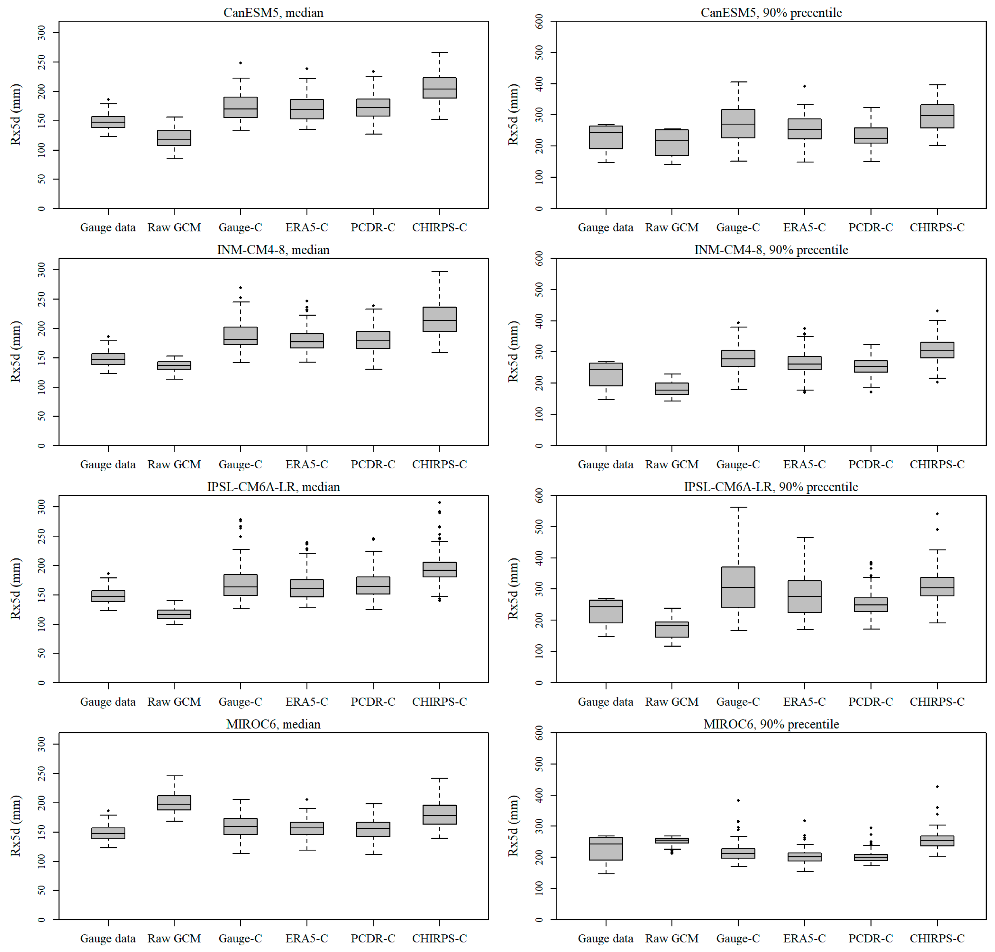
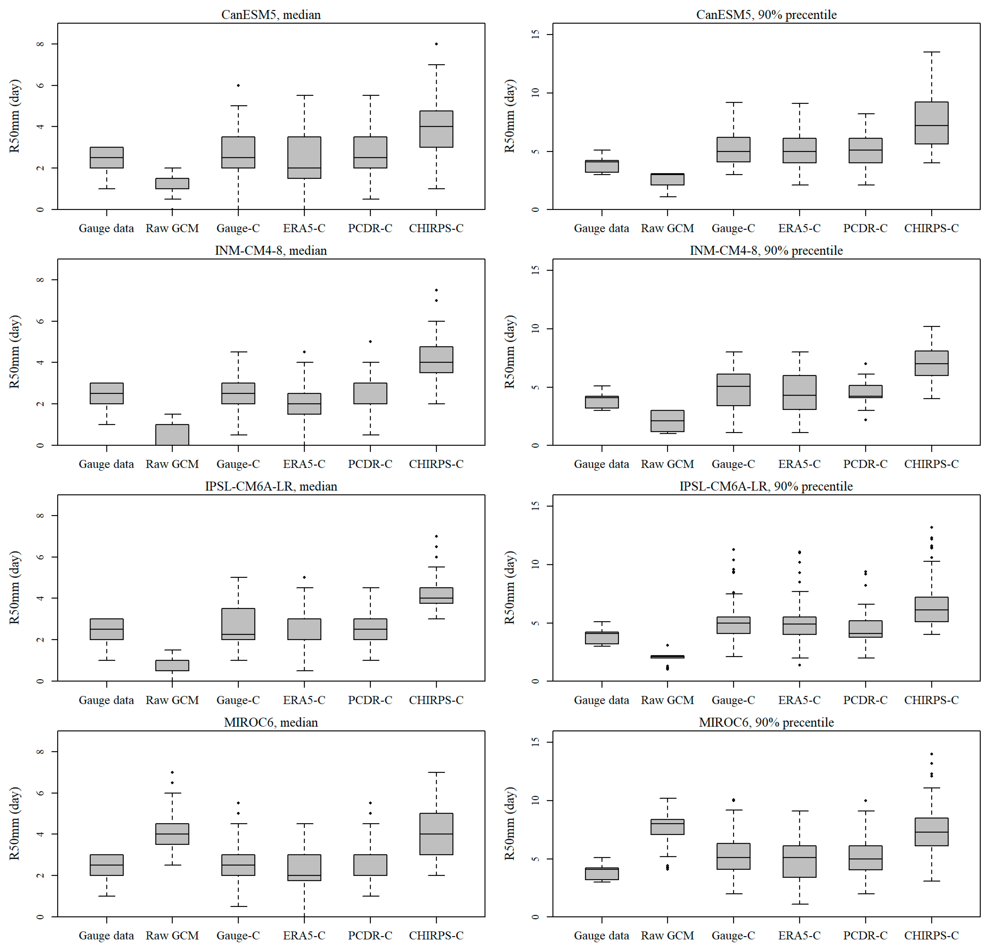
For the rainstorm-related extreme indices, the medians and high values (90% percentile) of Rx1d obtained from both the raw and bias-corrected GCM precipitation outputs are shown in Figure 6, while the results of Rx5d and R50mm are shown in Figure A2 and Figure A3 in Appendix A. In terms of the raw GCM precipitation output, most GCMs tend to underestimate the extreme indices, with the exception of MIROC, which tends to overestimate them. However, after applying bias-correction using QPEs as well as the gauge data, the extreme indices of all GCMs show overestimation for both medians and high values. Interestingly, despite the poor performance in reproducing overall precipitation intensity, the bias-correction results of ERA5 generally exhibit the best reproduction of extreme indices. ERA5 demonstrates smaller deviations in Rx1d, Rx5d, and R50mm compared to the gauge data, although overestimations are still present. On the other hand, the results obtained from PCDR show slightly poorer performance, with relatively larger deviations of extreme indices from the gauge data in more cases compared to ERA5. Notably, CHIRPS displays the poorest performance in bias-correcting GCMs for the reproduction of extreme rainstorm events, as its Rx1d and Rx5d values are significantly overestimated by up to about 50% to 100% for both medians and high values.
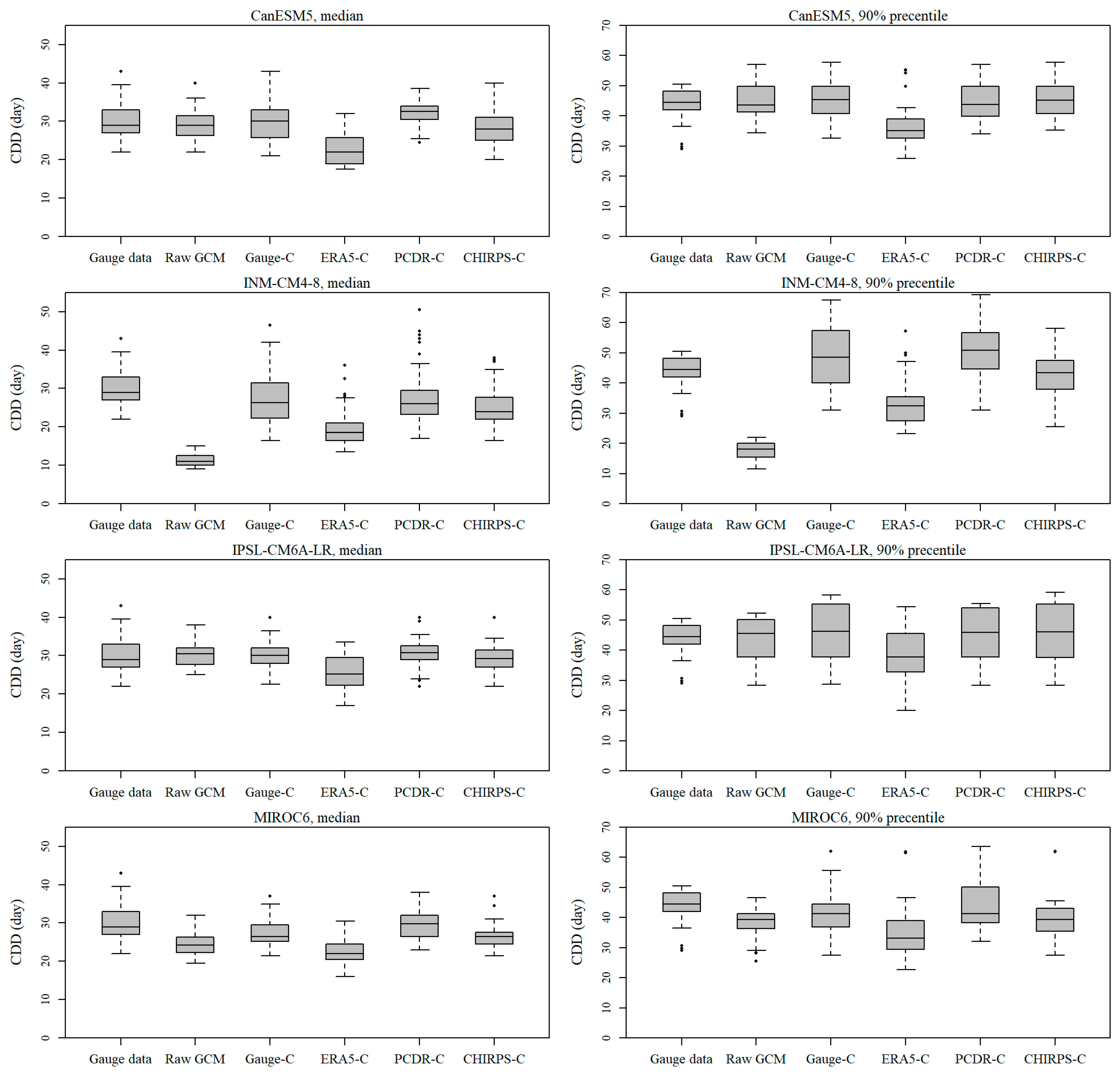
Figure 7 illustrates the medians and high values (90% percentile) of the drought-related extreme index, CDD, obtained from both the raw and bias-corrected GCM precipitation outputs. Longer CDDs typically indicate severer drought conditions. In the case of the raw GCM outputs, most GCMs exhibit a small deviation for CDD, except for INM-CM4-8, which shows significant underestimation of CDD for both medians and high values. This underestimation might be attributed to the overestimation of small precipitation events by this particular GCM. Upon applying bias-correction to the GCM outputs, the results obtained from PCDR and CHIRPS display relatively small deviations of CDD when compared to the gauge data. However, the bias-correction results from ERA5 indicate apparent underestimation of CDD.
In summary, in terms of bias-correction for GCM precipitation outputs, PCDR generally exhibits the best and most consistent performance. The bias-corrected GCM outputs using ERA5 tend to overestimate the overall precipitation amount while underestimating the CDD values; the bias-correction results obtained from CHIRPS tend to overestimate the rainstorm-related extreme indices.

4.3. Evaluation of Simulated Streamflow of GCM Precipitation Outputs Bias-Corrected by QPEs

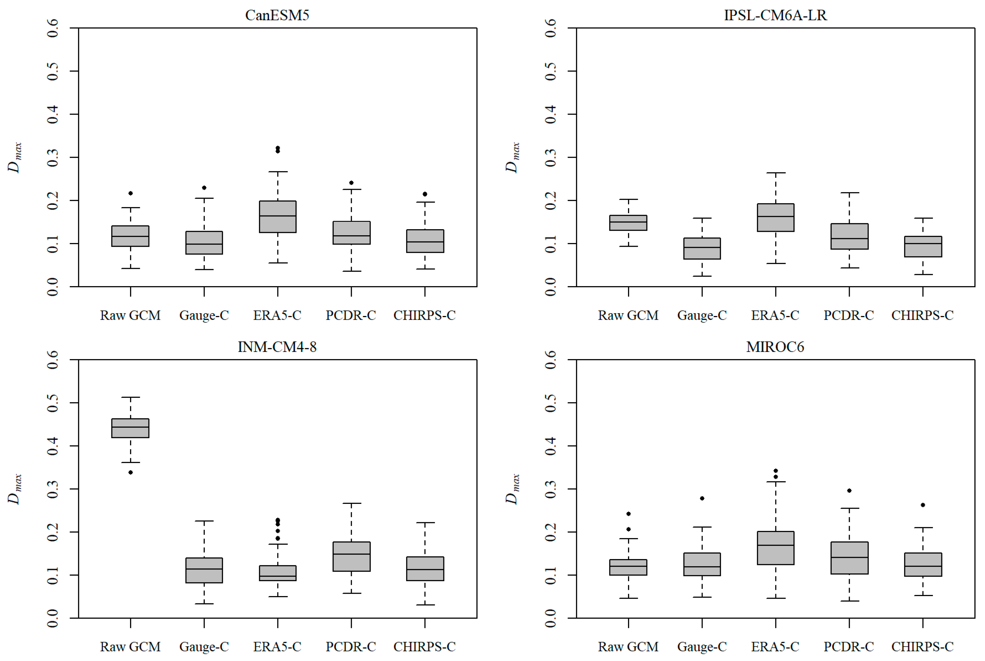
Figure 8 shows the D m a x values of the simulated streamflow obtained from both the raw and bias-corrected GCM precipitation outputs. The boxplots in the figure represent the distribution of D m a x values among the results of 100 sample sets. Regarding the raw GCM output, CanESM5 and MIROC6 exhibit a good fit to the distribution of simulated streamflow, as indicated by their low D m a x values. However, INM-CM4-8 demonstrates the highest D m a x value for simulated streamflow, which might be attributed to the substantial deviation of its precipitation outputs from reality. After applying bias-correction to the GCM outputs using QPEs, the results of CHIRPS demonstrate the smallest D m a x values among the three QPEs, indicating the most significant improvement in the overall distribution of the simulated streamflow. D m a x values of PCDR’s results generally rank second in terms of performance. Once again, the results of ERA5 exhibit the poorest performance, except for the case of INM-CM4-8, with high D m a x values for the simulated streamflow produced by the bias-corrected GCM outputs. This could be attributed to the less accurate distribution of ERA5-corrected precipitation outputs.
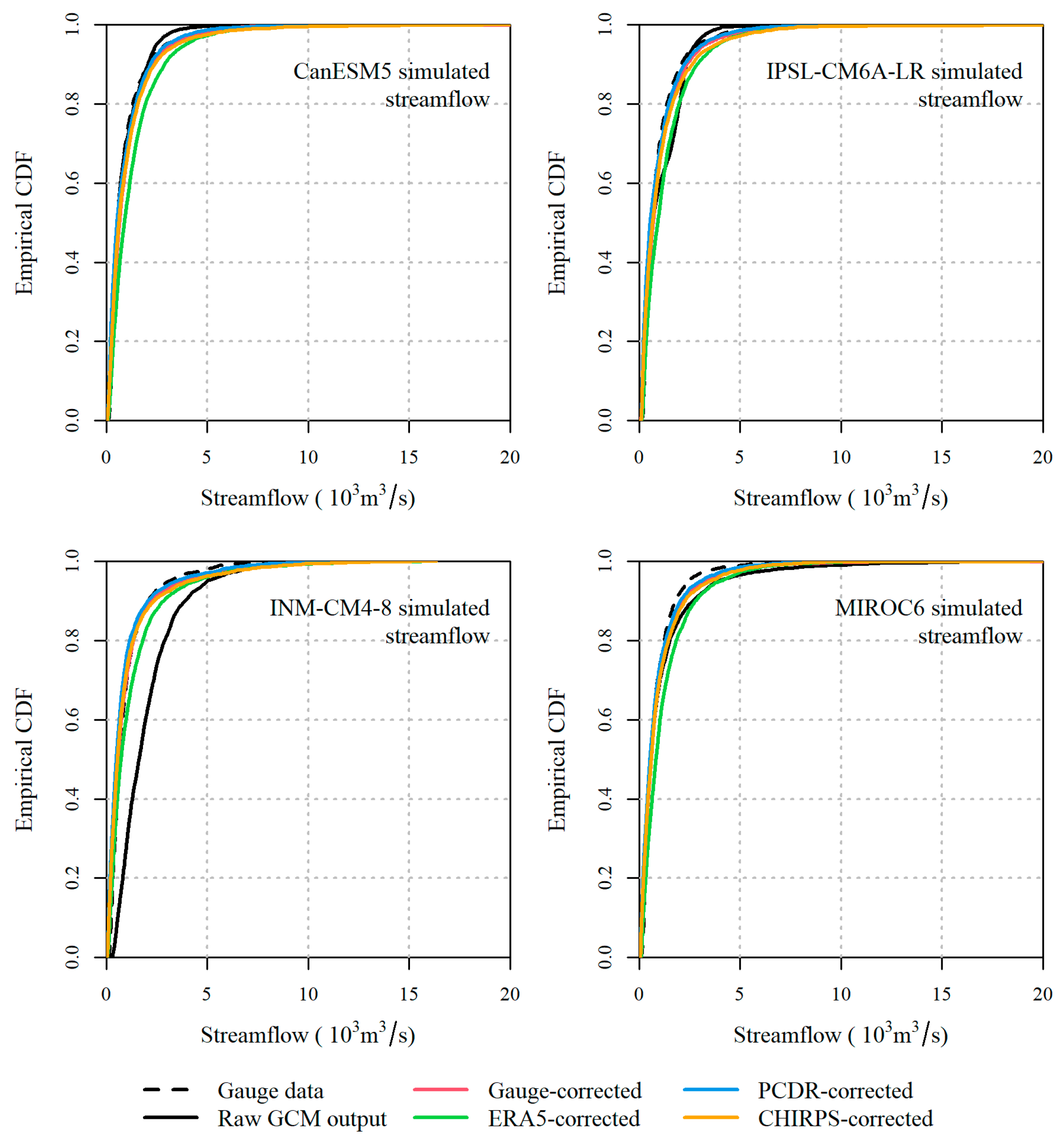
Figure 9 shows the empirical CDFs of the simulated streamflow obtained from both the raw and bias-corrected GCM precipitation outputs. These empirical CDFs were derived from the sample that has the median D m a x values of simulated streamflow among all 100 sample sets. Similar to the precipitation outputs, the raw GCM outputs for simulated streamflow exhibit noticeable deviations from the observed streamflow data in the empirical CDF curves. The shapes of these CDFs closely resemble those of the precipitation outputs. Notably, INM-CM4-8 shows significant overestimation for low and medium streamflow values (below 10 × 10 3   m 3 / s ). Again, the bias-corrected GCM outputs generally show improved agreement with the observed streamflow in terms of the empirical CDF curves. Both the PCDR and CHIRPS bias-correction results exhibit good fitness to the gauge data for all GCMs, while the ERA5 results show apparent overestimation for the simulated streamflow.
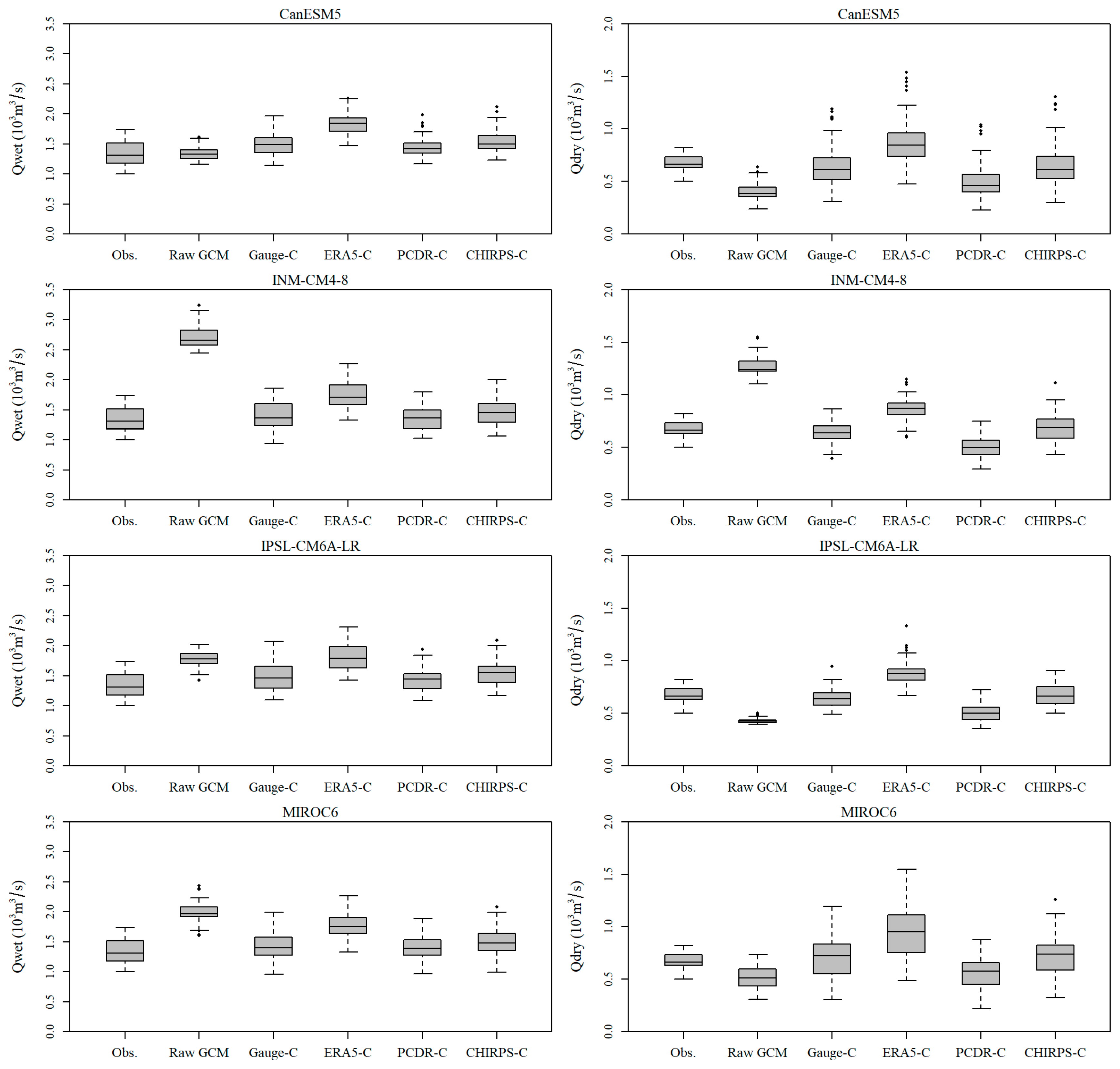
For the extreme indices related to overall streamflow (Qmean, Qwet, and Qdry), the median values of Qmeans simulated by the GCM precipitation outputs before and after bias-correction using QPEs are shown in Figure 10, while the results of Qwet and Qdry are shown in Figure A4 in Appendix A. The accuracy of the Qmeans by the raw and bias-corrected GCMs is similar to the results shown in Figure 6 for SDII. This similarity can be attributed to the close relationship between total precipitation and total streamflow within a single basin. INM-CM4-8 also demonstrates the most significant overestimation for Qmeans. Regarding the bias-corrected GCM results, similar to the SDII results, ERA5 still shows significant overestimation for Qmeans by up to about 30% (according to the medians of 100 sample sets). The reproduced Qmeans by the PCDR-corrected GCMs exhibit the least discrepancies compared to the observed streamflow, albeit with slight underestimation. The Qmeans of the CHIRPS-corrected GCMs show slightly larger deviations from the observed streamflow compared to the PCDR results and tend to show overestimation.
For Qwet and Qdry, regarding the simulated streamflow from the raw GCM outputs, CanESM5 accurately reproduces Qwet but underestimates Qdry. INM-CM4-8 shows significant overestimation for both Qwet and Qdry. IPSL-CM6A-LR and MIROC6 both overestimate Qwet but underestimate Qdry. After bias-correction by PCDR and CHIRPS, the reproduced Qwet and Qdry by the GCMs generally exhibit closer agreement with the observations. The PCDR-corrected results tend to underestimate Qdry, while CHIRPS tends to overestimate Qwet. Similar to the results of SDII and Qmean, the bias-correction results by ERA5 also show significant overestimation for both Qwet and Qdry.
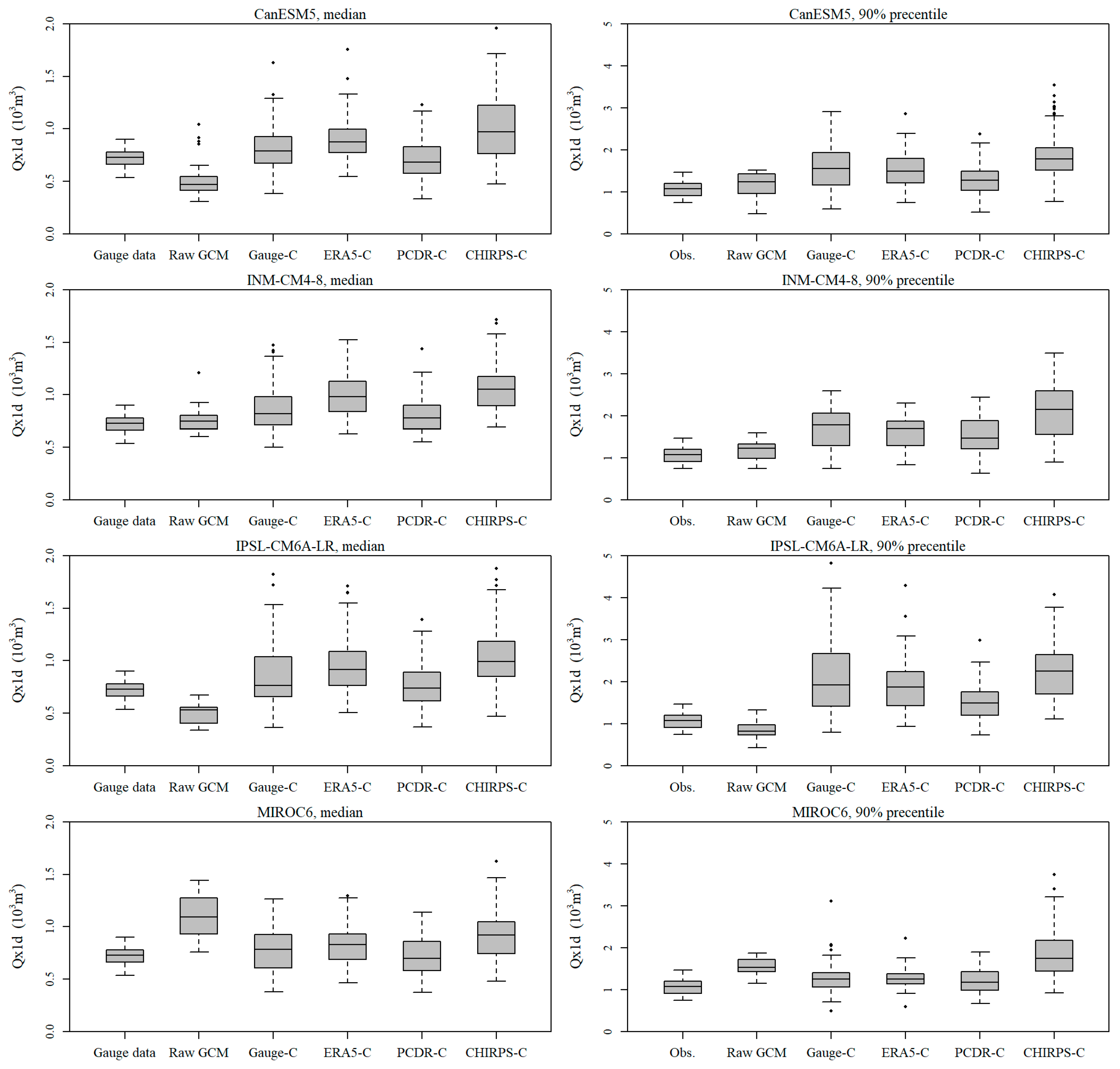
For the flood-related extreme indices, the medians and high values (at the 90% quantile) of Qx1d over the 10 years of “validation sets” obtained from both the raw and bias-corrected GCM precipitation outputs are shown in Figure 11, while the results of Qx5d are shown in Figure A5 in Appendix A. These indices serve as indicators for the reproduction of extreme flood events. In the case of the raw GCM precipitation output, CanESM5 and IPSL-CM6A-LR tend to underestimate both Qx1d and Qx5d, while INM-CM4-8 and MIROC6 tend to exhibit overestimation, albeit to a lesser extent.
Regarding the bias-corrected GCM outputs, similar to the results observed for Rx1d and Rx5d, the Qx1d and Qx5d values of all QPE-corrected GCMs generally show overestimation, especially for the high values of these indices. The PCDR-corrected GCMs generally demonstrate the best reproduction of Qx1d and Qx5d, as their values are closer to the observed streamflow. The results obtained from ERA5 display larger deviations compared to PCDR when reproducing the two flood-related extreme indices, despite ERA5 outperforming PCDR in reproducing Rx1d and Rx5d. The results obtained from CHIRPS exhibit the poorest performance, with the reproduced Qx1d and Qx5d values showing the largest overestimation in most cases, even over 100% according to the median of 100 sample sets, and larger than the overestimation in Rx1d and Rx5d.
Figure 12 illustrates the medians and low values (at the 10% percentile) of the extreme index related to river water drought, i.e., Qn7d, obtained from both the raw and bias-corrected GCM precipitation outputs. The 10% percentile is utilized because a smaller Qn7d value indicates a more severe drought condition. In the case of the raw GCM outputs, most GCMs exhibit a slight underestimation of Qn7d, while INM-CM4-8 demonstrates a significant overestimation of Qn7d for both the median and low values, thereby indicating an underestimation of the severity of extreme drought events. Regarding the bias-corrected GCM outputs, in contrast to the results observed for CDD, the correction results obtained from ERA5 showcase the closest reproduction of Qn7d when compared to the observed streamflow. Conversely, both PCDR and CHIRPS exhibit an underestimation of Qn7d, suggesting an overestimated drought severity. Considering that the calibrated GR4J model was found to produce underestimated low flow, the results of ERA5 might be caused by the compensation for the overestimation of precipitation of ERA5 by the GR4J model.
Overall, in the context of bias-correction for GCM outputs in streamflow simulation, PCDR generally demonstrates the best performance. The simulated streamflow consistently exhibits reasonable performance in reproducing the streamflow distribution and extreme indices. The results obtained from ERA5 display less accurate reproduction of the streamflow distribution and an overestimation of overall streamflow. The results derived from CHIRPS tend to overestimate extreme floods.

5. Discussion

Our results reveal that the performance of bias-corrected GCM precipitation outputs highly depends on the accuracy, particularly the bias, of the QPEs used as correction references. ERA5 demonstrates high correlation (R) and low RMSE for daily precipitation, outperforming PCDR and CHIRPS in this study. However, it exhibits a high systematic bias, resulting in poorer bias-correction results compared to the other two QPEs. Several studies, such as Jiang et al. [52], Islam and Cartwright [53], and Jiao et al. [54], have also found overestimation in overall precipitation by ERA5. Nevertheless, bias correction for GCM precipitation outputs aims to improve the reproduction of climatic characteristics of precipitation by GCMs, with less consideration given to the reproduction of temporal trends and variations in reality [23]. As a result, the systematic bias of QPEs plays a more significant role in bias-correction performance than correlation and RMSE. Therefore, ERA5 is outperformed by the two satellite-based QPEs in this study, which have undergone error-correction. It is important to note that the results of this study were derived from the southern subtropical monsoon area, and the performance of ERA5 may differ in the northern temperate areas, as several studies have shown higher accuracy of ERA5 in those regions. Nevertheless, when choosing suitable QPEs for GCM bias-correction, referencing evaluation results from published works, the systematic bias of ERA5 should be carefully considered [52,54]. The same attention should also be paid to satellite-based QPEs if they are corrected using ground-based gauge data, as the improvement in bias may depend largely on the density of the gauges used, such as the CHIRPS used in this study [55,56,57].
As shown in the results, PCDR demonstrates the most stable performance in bias-correction of GCM precipitation outputs. Even though the correction results by PCDR may not always show apparent superiority to other QPEs in all cases, they do not exhibit significant deviations from observations in terms of both reproduced distribution and extreme values. This indicates the applicability of PCDR for various purposes related to GCM-based future water resource projection, such as available water resource prediction, hydropower planning, and flood/drought disaster prediction. Zhu et al. [28] and Katiraie-Boroujerdy et al. [29] have also showed the reasonable performance of PCDR in improving the GCM outputs by bias-correction in different areas. Compared to these studies that only focus on PCDR, this study reveals more information about the differences of bias-correction utility between QPEs by comparing multiple QPEs. In comparison with PCDR, the results from ERA5 often show substantial overestimation in overall precipitation/streamflow, while CHIRPS shows significant overestimation in rainstorm/flood-related extreme indices. Some studies attribute the superiority of PCDR over other infrared-based satellite QPEs, such as CHIRPS, to the GPCP dataset used for error-correction of PCDR, which includes more satellite data sources, including microwave remote sensing [30,56]. PCDR has also already been used in climatical studies, including bias-correction of GCM outputs in previous studies [28,29,58,59], and it has been found suitable for substituting ground observations in ungauged areas [28]. However, these studies did not compare PCDR with other QPEs. One might wonder if there are QPEs more suitable than PCDR for certain aspects of GCM bias-correction, which is also addressed in this study. Our results not only further demonstrate the capability of PCDR for bias-correcting GCM precipitation outputs but also reveal discrepancies between PCDR and other QPEs in various aspects of GCM bias-correction, providing additional information for choosing suitable QPEs to meet the requirements of GCM-based water resource projection practices over ungauged areas.
Besides the PCDR, CHIRPS also has the potential to substitute gauge observations for GCM bias-correction, as it shows similar performance to PCDR, except for significant overestimations in rainstorm/flood-related extreme indices like Rx1d. Bias-corrected GCM precipitation by CHIRPS performs well in reproducing overall precipitation and drought-related indices, demonstrating the applicability of CHIRPS for GCM-based applications, including water resource planning and drought prediction. It is worth noting that CHIRPS has a much finer spatial resolution (0.05°) than PCDR and ERA5 [39], and PCDR has been found to have weaknesses in revealing the spatial pattern of precipitation [30,41]. Therefore, CHIRPS might be more suitable for practices requiring accurate spatial precipitation patterns.
Our results also reveal that the hydrological model might also influence the streamflow projection performance of bias-corrected GCMs. Zhu et al. [28] indicated that the modeled streamflow by GCMs generally has consistence with their behaviors in precipitation. Nevertheless, our results show that the GR4J model tends to produce smaller low flow than observations, enhancing the performance of bias-corrected GCMs in reproducing extreme low-flow events, even though the GR4J model performs satisfactorily in reproducing overall streamflow and peak values. This indicates that caution should be paid for the modeling performance of hydrological models for the considered aspects (like flood or drought projection). Moreover, our results also show that, for some occasions, the overestimation of flood-related extreme indices by corrected GCM via GR4J model is severer than the rainstorm-related extreme indices, especially for the cases of CHIRPS. Similarly, related studies [28,60] also pointed out that, due to the nonlinearities in hydrological process, the hydrological models have the potential to enlarge the error in precipitation inputs. As a result, attention should be paid that great improvement of GCM precipitation output after bias-correction is not necessary to produce the same effects on the streamflow simulations [28].

6. Conclusions

Under the global climate change background, it is urgent to develop reliable approaches to conduct bias-correction of GCM outputs and projection of future precipitation for the ungauged areas. To provide references for this issue, this study evaluated and compared the utility of three open-access long-term QPEs for bias-correcting GCM precipitation outputs. The evaluation included the assessments of precipitation distribution, streamflow simulation, and reproduced extreme indices for the bias-corrected GCM outputs. The quantile mapping (QM) approach, which bias-corrects the GCM outputs by establishing the statistical relationships between GCM outputs and historical observations like QPEs, was used to correct the GCM precipitation outputs based on QPEs. In total, 11 extreme indices were used as cases to evaluate the ability of GCM in reproducing extreme events after bias-correction. The main conclusions derived from this study are summarized as follows:
In terms of the performance of the QPEs themselves, both PCDR and CHIRPS exhibit satisfactory accuracy in precipitation estimation and streamflow simulation. However, ERA5 shows noticeable overestimation in precipitation amounts. PCDR demonstrates accurate reproduction of extreme indices related to floods and droughts, whereas ERA5 and CHIRPS exhibit significant overestimation.
When considering the raw GCM precipitation outputs, all GCMs demonstrate varying degrees of deviation in the statistical distribution of precipitation and streamflow, as well as in the reproduction of extreme indices compared to the observations. Notably, INM-CM4-8 exhibits substantial overestimation of overall precipitation and streamflow amounts, underestimation of drought severity indices, and underestimation of rainstorm-related extreme indices; MIROC6 underestimates flood-related extreme indices.
Regarding the bias-corrected GCM outputs, among the three QPEs, PCDR generally shows the most effective bias-correction utility for GCM outputs. It consistently demonstrates reasonable performance in reproducing the distribution of precipitation and streamflow, as well as the extreme indices in most cases. This suggests that PCDR is a suitable alternative to gauge data for bias-correction in remote and ungauged areas. Conversely, the GCM outputs corrected by ERA5 exhibit noticeable overestimation in the reproduction of overall precipitation and streamflow, while the correction results from CHIRPS significantly overestimate rainstorm/flood-related extreme indices.

Author Contributions

Conceptualization, D.C. and C.L.; methodology, D.C.; software, D.C.; validation, X.J., S.L. and F.C.; formal analysis, D.C.; investigation, D.C.; resources, C.L.; data curation, D.C.; writing—original draft preparation, D.C.; writing—review and editing, C.L.; visualization, Y.L.; supervision, C.L.; project administration, D.C. and C.L.; funding acquisition, C.L. All authors have read and agreed to the published version of the manuscript.

Funding

The Flood & Drought Disaster Prevention Capability Improvement Project of Sichuan Province (N5100012023000037); the Natural Science Foundation of Guangdong Province (2023B1515020087).

Institutional Review Board Statement

Not applicable.

Informed Consent Statement

Not applicable.

Data Availability Statement

Not applicable.

Conflicts of Interest

The authors declare no conflict of interest.

Abbreviations

CDFCumulated distribution functions
CHIRPSClimate Hazards Group (CHG) Infrared Precipitation with Station
CMIPCoupled Model Intercomparison Project
CMIP6CMIP phase 6
ERA5The fifth generation of European Centre for Medium-Range Weather
Forecasts (ECMWF) Reanalysis
GCMGlobal Climate Model
GR4JGénie Rural à 4 paramètres Journalier
K-S testKolmogorov–Smirnov test
KGEKling–Gupta efficiency coefficient
NSENash–Sutcliffe efficiency
PERSIANN-CDRPrecipitation Estimation from Remotely Sensed Information using
Artificial Neural Networks–Climate Data Record
QMQuantile mapping
QPEQuantitative precipitation estimation
RPearson correlation coefficient
RBRelative bias
RMSERoot mean square error
SCE-UAShuffled Complex Evolution-University of Arizona
WRCPWorld Climate Research Programme

Appendix A

Figure A1. Calibration results of the GR4J hydrological model. Note that the hydrographs are only used to illustrate the overall fitness of the modeled streamflow by calibrated hydrological model with observations.
Water 15 02906 g0a1
Figure A2. Comparison of the median (left column) and 90% percentile (right column) of Rx5d from gauge data and raw/bias-corrected GCM daily precipitation outputs. Note: the boxplots show the distribution of Rx5d from the 100 sample sets: in the boxplots, the upper and lower bounds of the box indicate the 75% and 25% percentiles, respectively, while the horizontal line inside represents the median. The upper and lower horizontal lines outside the box indicate the maximum and minimum values, respectively, and points outside the box represent outliers.
Water 15 02906 g0a2
Figure A3. Comparison of the median (left column) and 90% percentile (right column) of R50mm from gauge data and raw/bias-corrected GCM daily precipitation outputs. Note: the boxplots show the distribution of R50mm from the 100 sample sets: in the boxplots, the upper and lower bounds of the box indicate the 75% and 25% percentiles, respectively, while the horizontal line inside represents the median. The upper and lower horizontal lines outside the box indicate the maximum and minimum values, respectively, and points outside the box represent outliers.
Water 15 02906 g0a3
Figure A4. Comparison of the Qwet (left column) and Qdry (right column) of gauge data and raw/bias-corrected GCM daily precipitation outputs. Note: the boxplots show the distribution of Qwet/Qdry from the 100 sample sets: in the boxplots, the upper and lower bounds of the box indicate the 75% and 25% percentiles, respectively, while the horizontal line inside represents the median. The upper and lower horizontal lines outside the box indicate the maximum and minimum values, respectively, and points outside the box represent outliers.
Water 15 02906 g0a4
Figure A5. Comparison of the median (left column) and 90% percentile (right column) of Qx5d from gauge data and raw/bias-corrected GCM daily precipitation outputs. Note: the boxplots show the distribution of Qx5d from the 100 sample sets: in the boxplots, the upper and lower bounds of the box indicate the 75% and 25% percentiles, respectively, while the horizontal line inside represents the median. The upper and lower horizontal lines outside the box indicate the maximum and minimum values, respectively, and points outside the box represent outliers.
Water 15 02906 g0a5
Table A1. Comparison of hydrological extreme indices of observation data and calibration results of GR4J during 1985 to 2011. Note: the high value of Qx1d and Qx5d (representing flood) were illustrated by the 90% percentiles, while low values of Qn7d (representing drought) were illustrated by the 10% percentiles.
Extreme IndexQx1d (m3)Qx5d (m3)Qn7d (m3)
MedianObservation738.72438.9116.3
Modeled streamflow712.32581.677.7
90% percentile
(10% percentile for Qn7d)
Observation1132.34331.779.3
Modeled streamflow1185.94455.452.2

References

  1. Milly, P.C.D.; Betancourt, J.; Falkenmark, M.; Hirsch, R.M.; Kundzewicz, Z.W.; Lettenmaier, D.P.; Stouffer, R.J. Stationarity Is Dead: Whither Water Management? Science 2008, 319, 573–574. [Google Scholar] [CrossRef]
  2. Valjarević, A.; Milanović, M.; Gultepe, I.; Filipović, D.; Lukić, T. Updated Trewartha climate classification with four climate change scenarios. Geogr. J. 2022, 188, 506–517. [Google Scholar] [CrossRef]
  3. Madakumbura, G.D.; Thackeray, C.W.; Norris, J.; Goldenson, N.; Hall, A. Anthropogenic influence on extreme precipitation over global land areas seen in multiple observational datasets. Nat. Commun. 2021, 12, 3944. [Google Scholar] [CrossRef] [PubMed]
  4. Immerzeel, W.W.; Lutz, A.F.; Andrade, M.; Bahl, A.; Biemans, H.; Bolch, T.; Hyde, S.; Brumby, S.; Davies, B.J.; Elmore, A.C.; et al. Importance and vulnerability of the world’s water towers. Nature 2020, 577, 364–369. [Google Scholar] [CrossRef]
  5. Wang, Z.; Zhong, R.; Lai, C.; Chen, J. Evaluation of the GPM IMERG satellite-based precipitation products and the hydrological utility. Atmos. Res. 2017, 196, 151–163. [Google Scholar] [CrossRef]
  6. Zhong, R.; Zhao, T.; He, Y.; Chen, X. Hydropower change of the water tower of Asia in 21st century: A case of the Lancang River hydropower base, upper Mekong. Energy 2019, 179, 685–696. [Google Scholar] [CrossRef]
  7. Eyring, V.; Bony, S.; Meehl, G.A.; Senior, C.A.; Stevens, B.; Stouffer, R.J.; Taylor, K.E. Overview of the Coupled Model Intercomparison Project Phase 6 (CMIP6) experimental design and organization. Geosci. Model. Dev. 2016, 9, 1937–1958. [Google Scholar] [CrossRef] [Green Version]
  8. Knutti, R.; Masson, D.; Gettelman, A. Climate model genealogy: Generation CMIP5 and how we got there. Geophys. Res. Lett. 2013, 40, 1194–1199. [Google Scholar] [CrossRef]
  9. Eyring, V.; Cox, P.M.; Flato, G.M.; Gleckler, P.J.; Abramowitz, G.; Caldwell, P.; Collins, W.D.; Gier, B.K.; Hall, A.D.; Hoffman, F.M.; et al. Taking climate model evaluation to the next level. Nat. Clim. Chang. 2019, 9, 102–110. [Google Scholar] [CrossRef] [Green Version]
  10. Satoh, Y.; Yoshimura, K.; Pokhrel, Y.; Kim, H.; Shiogama, H.; Yokohata, T.; Hanasaki, N.; Wada, Y.; Burek, P.; Byers, E.; et al. The timing of unprecedented hydrological drought under climate change. Nat. Commun. 2022, 13, 3287. [Google Scholar] [CrossRef]
  11. Pokhrel, Y.; Felfelani, F.; Satoh, Y.; Boulange, J.; Burek, P.; Gädeke, A.; Gerten, D.; Gosling, S.N.; Grillakis, M.; Gudmundsson, L.; et al. Global terrestrial water storage and drought severity under climate change. Nat. Clim. Chang. 2021, 11, 226–233. [Google Scholar] [CrossRef]
  12. Boulange, J.; Hanasaki, N.; Yamazaki, D.; Pokhrel, Y. Role of dams in reducing global flood exposure under climate change. Nat. Commun. 2021, 12, 417. [Google Scholar] [CrossRef]
  13. Wing, O.E.J.; Lehman, W.; Bates, P.D.; Sampson, C.C.; Quinn, N.; Smith, A.M.; Neal, J.C.; Porter, J.R.; Kousky, C. Inequitable patterns of US flood risk in the Anthropocene. Nat. Clim. Chang. 2022, 12, 156–162. [Google Scholar] [CrossRef]
  14. Barbarossa, V.; Bosmans, J.; Wanders, N.; King, H.; Bierkens, M.F.P.; Huijbregts, M.A.J.; Schipper, A.M. Threats of global warming to the world’s freshwater fishes. Nat. Commun. 2021, 12, 1701. [Google Scholar] [CrossRef]
  15. Xi, Y.; Peng, S.; Ciais, P.; Chen, Y. Future impacts of climate change on inland Ramsar wetlands. Nat. Clim. Chang. 2021, 11, 45–51. [Google Scholar] [CrossRef]
  16. Gernaat, D.E.H.J.; de Boer, H.S.; Daioglou, V.; Yalew, S.G.; Müller, C.; van Vuuren, D.P. Climate change impacts on renewable energy supply. Nat. Clim. Chang. 2021, 11, 119–125. [Google Scholar] [CrossRef]
  17. Zhong, R.; Zhao, T.; Chen, X. Evaluating the tradeoff between hydropower benefit and ecological interest under climate change: How will the water-energy-ecosystem nexus evolve in the upper Mekong basin? Energy 2021, 237, 121518. [Google Scholar] [CrossRef]
  18. O’Neill, B.C.; Tebaldi, C.; van Vuuren, D.P.; Eyring, V.; Friedlingstein, P.; Hurtt, G.; Knutti, R.; Kriegler, E.; Lamarque, J.F.; Lowe, J.; et al. The Scenario Model Intercomparison Project (ScenarioMIP) for CMIP6. Geosci. Model. Dev. 2016, 9, 3461–3482. [Google Scholar] [CrossRef] [Green Version]
  19. Gupta, V.; Singh, V.; Jain, M.K. Assessment of precipitation extremes in India during the 21st century under SSP1-1.9 mitigation scenarios of CMIP6 GCMs. J. Hydrol. 2020, 590, 125422. [Google Scholar] [CrossRef]
  20. Hempel, S.; Frieler, K.; Warszawski, L.; Schewe, J.; Piontek, F. A trend-preserving bias correction—The ISI-MIP approach. Earth Syst. Dynam 2013, 4, 219–236. [Google Scholar] [CrossRef] [Green Version]
  21. Mishra, V.; Bhatia, U.; Tiwari, A.D. Bias-corrected climate projections for South Asia from Coupled Model Intercomparison Project-6. Sci. Data 2020, 7, 338. [Google Scholar] [CrossRef] [PubMed]
  22. Ehret, U.; Zehe, E.; Wulfmeyer, V.; Warrach-Sagi, K.; Liebert, J. HESS Opinions “Should we apply bias correction to global and regional climate model data”? Hydrol. Earth Syst. Sci. 2012, 16, 3391–3404. [Google Scholar] [CrossRef] [Green Version]
  23. Stefanidis, S.; Dafis, S.; Stathis, D. Evaluation of Regional Climate Models (RCMs) Performance in Simulating Seasonal Precipitation over Mountainous Central Pindus (Greece). Water 2020, 12, 2750. [Google Scholar] [CrossRef]
  24. Tolika, K.; Anagnostopoulou, C.; Maheras, P.; Vafiadis, M. Simulation of future changes in extreme rainfall and temperature conditions over the Greek area: A comparison of two statistical downscaling approaches. Glob. Planet. Chang. 2008, 63, 132–151. [Google Scholar] [CrossRef]
  25. Brighenti, T.M.; Gassman, P.W.; Gutowski, W.J.; Thompson, J.R. Assessing the Influence of a Bias Correction Method on Future Climate Scenarios Using SWAT as an Impact Model Indicator. Water 2023, 15, 750. [Google Scholar] [CrossRef]
  26. Pan, H.; Jin, Y.; Zhu, X. Comparison of Projections of Precipitation over Yangtze River Basin of China by Different Climate Models. Water 2022, 14, 1888. [Google Scholar] [CrossRef]
  27. Derdour, S.; Ghenim, A.N.; Megnounif, A.; Tangang, F.; Chung, J.X.; Ayoub, A.B. Bias Correction and Evaluation of Precipitation Data from the CORDEX Regional Climate Model for Monitoring Climate Change in the Wadi Chemora Basin (Northeastern Algeria). Atmosphere 2022, 13, 1876. [Google Scholar] [CrossRef]
  28. Zhu, Q.; Hsu, K.; Xu, Y.; Yang, T. Evaluation of a new satellite-based precipitation data set for climate studies in the Xiang River basin, southern China. Int. J. Climatol. 2017, 37, 4561–4575. [Google Scholar] [CrossRef]
  29. Katiraie-Boroujerdy, P.; Akbari Asanjan, A.; Chavoshian, A.; Hsu, K.; Sorooshian, S. Assessment of seven CMIP5 model precipitation extremes over Iran based on a satellite-based climate data set. Int. J. Climatol. 2019, 39, 3505–3522. [Google Scholar] [CrossRef]
  30. Bai, X.; Wu, X.; Wang, P. Blending long-term satellite-based precipitation data with gauge observations for drought monitoring: Considering effects of different gauge densities. J. Hydrol. 2019, 577, 124007. [Google Scholar] [CrossRef]
  31. Wang, P.; Bai, X.; Wu, X.; Lai, C.; Zhang, Z. Spatially continuous assessment of satellite-based precipitation products using triple collocation approach and discrete gauge observations via geographically weighted regression. J. Hydrol. 2022, 608, 127640. [Google Scholar] [CrossRef]
  32. Huffman, G.J.; Bolvin, D.T.; Nelkin, E.J.; Wolff, D.B.; Adler, R.F.; Gu, G.; Hong, Y.; Bowman, K.P.; Stocker, E.F. The TRMM Multisatellite Precipitation Analysis (TMPA): Quasi-Global, Multiyear, Combined-Sensor Precipitation Estimates at Fine Scales. J. Hydrometeorol. 2007, 8, 38–55. [Google Scholar] [CrossRef]
  33. Joyce, R.J.; Janowiak, J.E.; Arkin, P.A.; Xie, P. CMORPH: A Method that Produces Global Precipitation Estimates from Passive Microwave and Infrared Data at High Spatial and Temporal Resolution. J. Hydrometeorol. 2004, 5, 487–503. [Google Scholar] [CrossRef]
  34. Huffman, G.J.; Bolvin, D.T.; Braithwaite, D.; Hsu, K.; Joyce, R.J.; Kidd, C.; Nelkin, E.J.; Sorooshian, S.; Stocker, E.F.; Tan, J.; et al. Integrated Multi-satellite Retrievals for the Global Precipitation Measurement (GPM) Mission (IMERG). In Satellite Precipitation Measurement; Levizzani, V., Kidd, C., Kirschbaum, D.B., Kummerow, C.D., Nakamura, K., Turk, F.J., Eds.; Springer International Publishing: Cham, Switzerland, 2020; Volume 1, pp. 343–353. [Google Scholar]
  35. Boucher, O.; Servonnat, J.; Albright, A.L.; Aumont, O.; Balkanski, Y.; Bastrikov, V.; Bekki, S.; Bonnet, R.; Bony, S.; Bopp, L.; et al. Presentation and Evaluation of the IPSL-CM6A-LR Climate Model. J. Adv. Model. Earth Syst. 2020, 12, e2010M–e2019M. [Google Scholar] [CrossRef]
  36. Hersbach, H.; Bell, B.; Berrisford, P.; Hirahara, S.; Horányi, A.; Muñoz-Sabater, J.; Nicolas, J.; Peubey, C.; Radu, R.; Schepers, D.; et al. The ERA5 global reanalysis. Q. J. R. Meteor. Soc. 2020, 146, 1999–2049. [Google Scholar] [CrossRef]
  37. Hong, Y.; Hsu, K.; Sorooshian, S.; Gao, X. Precipitation Estimation from Remotely Sensed Imagery Using an Artificial Neural Network Cloud Classification System. J. Appl. Meteorol. 2004, 43, 1834–1853. [Google Scholar] [CrossRef] [Green Version]
  38. Ashouri, H.; Hsu, K.; Sorooshian, S.; Braithwaite, D.K.; Knapp, K.R.; Cecil, L.D.; Nelson, B.R.; Prat, O.P. PERSIANN-CDR: Daily Precipitation Climate Data Record from Multisatellite Observations for Hydrological and Climate Studies. Bull. Am. Meteorol. Soc. 2015, 96, 69–83. [Google Scholar] [CrossRef] [Green Version]
  39. Funk, C.; Peterson, P.; Landsfeld, M.; Pedreros, D.; Verdin, J.; Shukla, S.; Husak, G.; Rowland, J.; Harrison, L.; Hoell, A.; et al. The climate hazards infrared precipitation with stations—A new environmental record for monitoring extremes. Sci. Data 2015, 2, 150066. [Google Scholar] [CrossRef] [Green Version]
  40. Lai, C.; Zhong, R.; Wang, Z.; Wu, X.; Chen, X.; Wang, P.; Lian, Y. Monitoring hydrological drought using long-term satellite-based precipitation data. Sci. Total Environ. 2019, 649, 1198–1208. [Google Scholar] [CrossRef]
  41. Zhong, R.; Zhao, T.; Chen, X.; Jin, H. Monitoring drought in ungauged areas using satellite altimetry: The Standardized River Stage Index. J. Hydrol. 2022, 612, 128308. [Google Scholar] [CrossRef]
  42. Babaousmail, H.; Hou, R.; Ayugi, B.; Sian, K.T.C.L.; Ojara, M.; Mumo, R.; Chehbouni, A.; Ongoma, V. Future changes in mean and extreme precipitation over the Mediterranean and Sahara regions using bias-corrected CMIP6 models. Int. J. Climatol. 2022, 42, 7280–7297. [Google Scholar] [CrossRef]
  43. Swart, N.C.; Cole, J.N.S.; Kharin, V.V.; Lazare, M.; Scinocca, J.F.; Gillett, N.P.; Anstey, J.; Arora, V.; Christian, J.R.; Hanna, S.; et al. The Canadian Earth System Model version 5 (CanESM5.0.3). Geosci. Model. Dev. 2019, 12, 4823–4873. [Google Scholar] [CrossRef] [Green Version]
  44. Volodin, E. The Mechanisms of Cloudiness Evolution Responsible for Equilibrium Climate Sensitivity in Climate Model INM-CM4-8. Geophys. Res. Lett. 2021, 48, e2021G–e96204G. [Google Scholar] [CrossRef]
  45. Ando, T.; Higuchi, T.; Hotta, H.; Iwakiri, T.; Jinno, T.; Kino, K.; Takano, Y.; Toda, M.; Yamazaki, K.; Suzuki, K.S. Description of MIROC6 AGCM; The University of Tokyo: Chiba, Japan, 2021. [Google Scholar]
  46. Cannon, A.J.; Sobie, S.R.; Murdock, T.Q. Bias Correction of GCM Precipitation by Quantile Mapping: How Well Do Methods Preserve Changes in Quantiles and Extremes? J. Clim. 2015, 28, 6938–6959. [Google Scholar] [CrossRef]
  47. Gupta, H.V.; Kling, H.; Yilmaz, K.K.; Martinez, G.F. Decomposition of the mean squared error and NSE performance criteria: Implications for improving hydrological modelling. J. Hydrol. 2009, 377, 80–91. [Google Scholar] [CrossRef] [Green Version]
  48. Birnbaum, Z.W.; Tingey, F.H. One-Sided Confidence Contours for Probability Distribution Functions. Ann. Math. Stat. 1951, 22, 592–596. [Google Scholar] [CrossRef]
  49. Perrin, C.; Michel, C.; Andréassian, V. Improvement of a parsimonious model for streamflow simulation. J. Hydrol. 2003, 279, 275–289. [Google Scholar] [CrossRef]
  50. Cao, D.; Li, H.; Hou, E.; Song, S.; Lai, C. Assessment and Hydrological Validation of Merged Near-Real-Time Satellite Precipitation Estimates Based on the Gauge-Free Triple Collocation Approach. Remote Sens. 2022, 14, 3835. [Google Scholar]
  51. Duan, Q.; Sorooshian, S.; Gupta, V. Effective and efficient global optimization for conceptual rainfall-runoff models. Water Resour. Res. 1992, 28, 1015–1031. [Google Scholar] [CrossRef]
  52. Jiang, Q.; Li, W.; Fan, Z.; He, X.; Sun, W.; Chen, S.; Wen, J.; Gao, J.; Wang, J. Evaluation of the ERA5 reanalysis precipitation dataset over Chinese Mainland. J. Hydrol. 2021, 595, 125660. [Google Scholar] [CrossRef]
  53. Islam, M.A.; Cartwright, N. Evaluation of climate reanalysis and space-borne precipitation products over Bangladesh. Hydrol. Sci. J. 2020, 65, 1112–1128. [Google Scholar] [CrossRef]
  54. Jiao, D.; Xu, N.; Yang, F.; Xu, K. Evaluation of spatial-temporal variation performance of ERA5 precipitation data in China. Sci. Rep. 2021, 11, 17956. [Google Scholar] [CrossRef]
  55. Zhong, R.; Chen, X.; Lai, C.; Wang, Z.; Lian, Y.; Yu, H.; Wu, X. Drought monitoring utility of satellite-based precipitation products across mainland China. J. Hydrol. 2019, 568, 343–359. [Google Scholar] [CrossRef]
  56. Bai, X.; Wang, P.; He, Y.; Zhang, Z.; Wu, X. Assessing the accuracy and drought utility of long-term satellite-based precipitation estimation products using the triple collocation approach. J. Hydrol. 2021, 603, 127098. [Google Scholar] [CrossRef]
  57. Bai, X.; Shen, W.; Wu, X.; Wang, P. Applicability of long-term satellite-based precipitation products for drought indices considering global warming. J. Environ. Manag. 2020, 255, 109846. [Google Scholar] [CrossRef]
  58. Ombadi, M.; Nguyen, P.; Sorooshian, S.; Hsu, K. Retrospective Analysis and Bayesian Model Averaging of CMIP6 Precipitation in the Nile River Basin. J. Hydrometeorol. 2021, 22, 217–229. [Google Scholar] [CrossRef]
  59. Lavers, D.A.; Simmons, A.; Vamborg, F.; Rodwell, M.J. An evaluation of ERA5 precipitation for climate monitoring. Q. J. R. Meteor. Soc. 2022, 148, 3152–3165. [Google Scholar] [CrossRef]
  60. Zhu, Q.; Xuan, W.; Liu, L.; Xu, Y. Evaluation and hydrological application of precipitation estimates derived from PERSIANN-CDR, TRMM 3B42V7, and NCEP-CFSR over humid regions in China. Hydrol. Process 2016, 30, 3061–3083. [Google Scholar] [CrossRef]
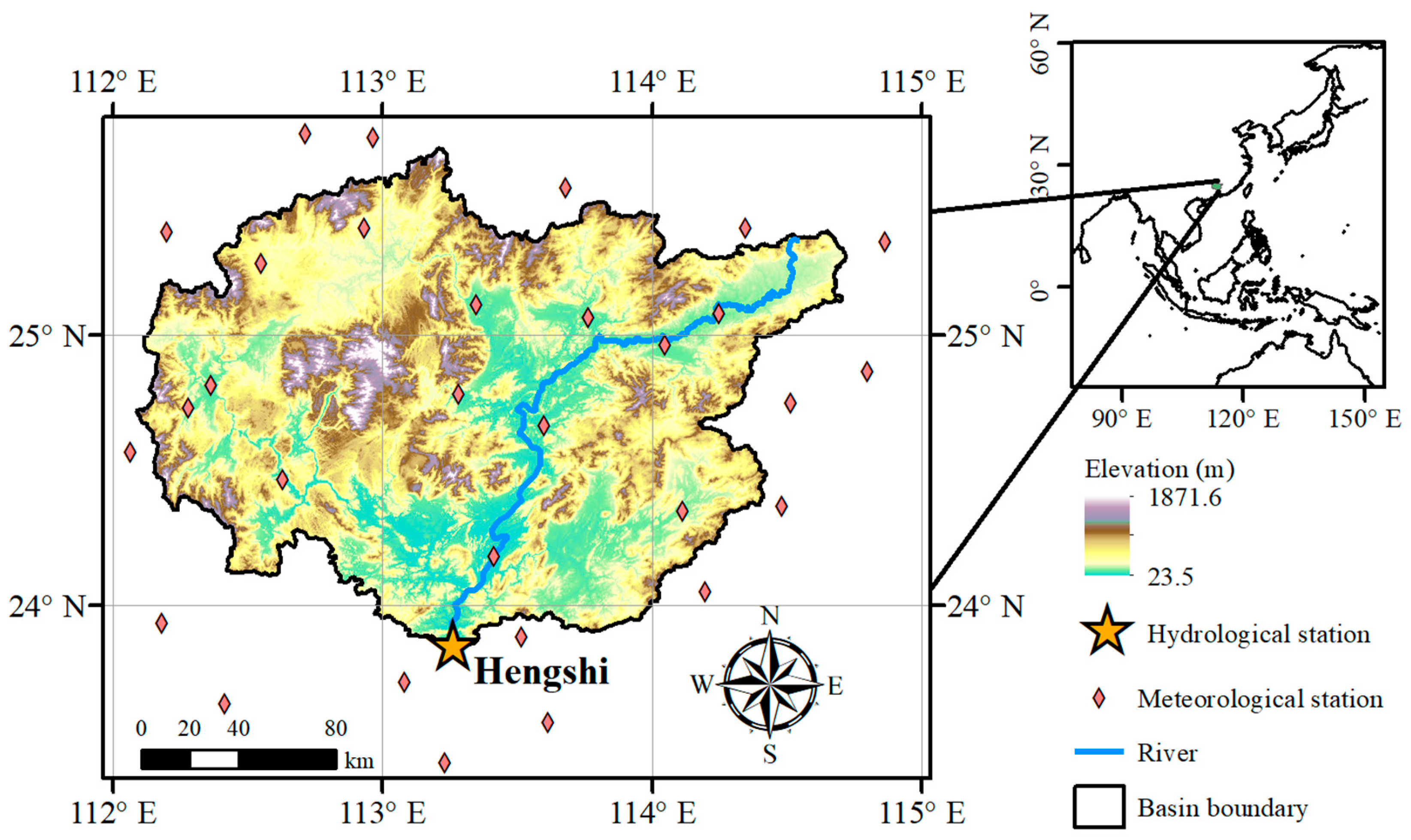
Figure 1. Geographical location and spatial distribution of meteorological and hydrological stations of the Beijiang basin.
Water 15 02906 g001
Figure 2. Flowchart of the evaluation of QPEs’ utility for bias-correction in this study.
Water 15 02906 g002
Figure 3. D m a x of the K-S test for raw and bias-corrected GCM daily precipitation outputs. Note: Gauge-C, ERA5-C, PCDR-C, and CHIRPS-C determine the outputs bias-corrected by gauge data, ERA5, PCDR, and CHIRPS; the boxplots show the distribution of D m a x from the 100 sample sets: in the boxplots, the upper and lower bounds of the box indicate the 75% and 25% percentiles, respectively, while the horizontal line inside represents the median. The upper and lower horizontal lines outside the box indicate the maximum and minimum values, respectively, and points outside the box represent outliers.
Water 15 02906 g003
Figure 4. Comparison of empirical cumulative distribution function (CDF) of the raw and bias-corrected GCM daily precipitation outputs.
Water 15 02906 g004
Figure 5. Comparison of the median SDII of gauge data and raw/bias-corrected GCM daily precipitation outputs. Note: the boxplots show the distribution of SDII from the 100 sample sets: in the boxplots, the upper and lower bounds of the box indicate the 75% and 25% percentiles, respectively, while the horizontal line inside represents the median. The upper and lower horizontal lines outside the box indicate the maximum and minimum values, respectively, and points outside the box represent outliers.
Water 15 02906 g005
Figure 6. Comparison of the median (left column) and 90% percentile (right column) of Rx1d from gauge data and raw/bias-corrected GCM daily precipitation outputs. Note: the boxplots show the distribution of Rx1d from the 100 sample sets: in the boxplots, the upper and lower bounds of the box indicate the 75% and 25% percentiles, respectively, while the horizontal line inside represents the median. The upper and lower horizontal lines outside the box indicate the maximum and minimum values, respectively, and points outside the box represent outliers.
Water 15 02906 g006
Figure 7. Comparison of the median (left column) and 90% percentile (right column) of CDD from gauge data and raw/bias-corrected GCM daily precipitation outputs. Note: the boxplots show the distribution of CDD from the 100 sample sets: in the boxplots, the upper and lower bounds of the box indicate the 75% and 25% percentiles, respectively, while the horizontal line inside represents the median. The upper and lower horizontal lines outside the box indicate the maximum and minimum values, respectively, and points outside the box represent outliers.
Water 15 02906 g007
Figure 8. D m a x of the K-S test for simulated daily streamflow from raw and bias-corrected GCM precipitation outputs. Note: the boxplots show the distribution of D m a x from the 100 sample sets: in the boxplots, the upper and lower bounds of the box indicate the 75% and 25% percentiles, respectively, while the horizontal line inside represents the median. The upper and lower horizontal lines outside the box indicate the maximum and minimum values, respectively, and points outside the box represent outliers.
Water 15 02906 g008
Figure 9. Comparison of empirical cumulative distribution function (CDF) of the simulated daily streamflow from raw and bias-corrected GCM precipitation outputs.
Water 15 02906 g009
Figure 10. Comparison of the Qmean of gauge data and raw/bias-corrected GCM daily precipitation outputs. Note: the boxplots show the distribution of Qmean from the 100 sample sets: in the boxplots, the upper and lower bounds of the box indicate the 75% and 25% percentiles, respectively, while the horizontal line inside represents the median. The upper and lower horizontal lines outside the box indicate the maximum and minimum values, respectively, and points outside the box represent outliers.
Water 15 02906 g010
Figure 11. Comparison of the median (left column) and 90% percentile (right column) of Qx1d from gauge data and raw/bias-corrected GCM daily precipitation outputs. Note: the boxplots show the distribution of Qx1d from the 100 sample sets: in the boxplots, the upper and lower bounds of the box indicate the 75% and 25% percentiles, respectively, while the horizontal line inside represents the median. The upper and lower horizontal lines outside the box indicate the maximum and minimum values, respectively, and points outside the box represent outliers.
Water 15 02906 g011
Figure 12. Comparison of the median (left column) and 10% percentile (right column) of Qn7d from gauge data and raw/bias-corrected GCM daily precipitation outputs. Note: the boxplots show the distribution of Qn7d from the 100 sample sets: in the boxplots, the upper and lower bounds of the box indicate the 75% and 25% percentiles, respectively, while the horizontal line inside represents the median. The upper and lower horizontal lines outside the box indicate the maximum and minimum values, respectively, and points outside the box represent outliers.
Water 15 02906 g012
Table 1. Information of the 4 CMIP6 GCMs used in this study.
GCMsInstituteSpatial Resolution
(Longitude × Latitude)
CanESM5Canadian Centre for Climate Modelling and Analysis2.8° × 2.8°
INM-CM4-8Marchuk Institute of Numerical Mathematics, Russian Academy of Science2° × 1.5°
IPSL-CM6A-LRInstitut Pierre-Simon Laplace2.5° × 1.25°
MIROC6Atmosphere and Ocean
Research Institute, University of Tokyo
1.4° × 1.4°
Table 2. Extreme indices used for evaluation of the climate utility of QPEs.
CategoryIndexDefinitionUnit
PrecipitationSDIIAnnual daily precipitation amount on wet days (precipitation ≥ 1 mm)mm
Rx1dMaximum 1-day precipitation of a yearmm
Rx5dMaximum consecutive 5-day precipitation of a yearmm
R50mmAnnual count of rainstorm days (precipitation ≥ 50 mm)day
CDDAnnual maximum number of consecutive dry days (precipitation < 1 mm)day
HydrologyQmeanMean annual streamflowm3/s
QwetWet season (April–September) mean streamflowm3/s
QdryDry season (October–March) mean streamflowm3/s
Qx1dMaximum 1-day flood water of a yearm3
Qx5dMaximum consecutive 5-day flood water of a yearm3
Qn7dMinimum consecutive 7-day streamflow of a yearm3
Table 3. Assessment metrics of the QPE daily and monthly precipitation.
Assessment MetricsRRMSE (mm)RB (%)
Daily scaleERA50.835.416.8
PCDR0.687.3−4.8
CHIRPS0.727.63.1
Monthly scaleERA50.9348.216.8
PCDR0.9437.3−4.8
CHIRPS0.9630.33.1
Table 4. Assessment metrics of the simulated daily streamflow by the QPEs.
PeriodAssessment MetricsGauge DataERA5PCDRCHIRPS
Calibration period
(1985–2000)
KGE0.960.490.780.85
R0.960.840.800.85
NSE0.920.420.630.70
RB (%)0.341.1−6.13.1
Calibration period
(2001–2011)
KGE0.920.810.780.80
R0.930.880.820.85
NSE0.860.740.670.66
RB (%)3.114.4−8.310.6
Table 5. Comparison of meteorological extreme indices calculated from gauge data and QPEs.
Extreme IndexRx1d (mm)Rx5d (mm)R50mm (day)CDD (day)
MedianGauge data73.8147.9329.5
ERA567150.7221.5
PCDR74161.5228
CHIRPS89.5165.5420
90% percentileGauge data93.6249.5448
ERA582.9197.5435.6
PCDR111212.1442.1
CHIRPS131.9239.9724
Table 6. Comparison of hydrological extreme indices of observation data and simulations by QPEs.
Extreme IndexQx1d (m3)Qx5d (m3)Qn7d (m3)
MedianObservation738.72438.9116.3
Gauge data712.32581.677.7
ERA5840.33131.993.4
PCDR719.52541.667.3
CHIRPS787.9253387.7
90% percentile
(10% percentile for Qn7d)
Observation1132.34331.779.3
Gauge data1185.94455.452.2
ERA51184.53932.164.5
PCDR1069.33581.750.7
CHIRPS1427.14239.564.3
Disclaimer/Publisher’s Note: The statements, opinions and data contained in all publications are solely those of the individual author(s) and contributor(s) and not of MDPI and/or the editor(s). MDPI and/or the editor(s) disclaim responsibility for any injury to people or property resulting from any ideas, methods, instructions or products referred to in the content.