Article

Encoder–Decoder Convolutional Neural Networks for Flow Modeling in Unsaturated Porous Media: Forward and Inverse Approaches

by
Mohammad Reza Hajizadeh Javaran
1,
Mohammad Mahdi Rajabi
1,*,
Nima Kamali
1,
Marwan Fahs
2 and
Benjamin Belfort
2
1
Civil and Environmental Engineering Faculty, Tarbiat Modares University, Tehran 14115-397, Iran
2
Université de Strasbourg, CNRS, ENGEES, EOST, ITES UMR 7063, F-67000 Strasbourg, France
*
Author to whom correspondence should be addressed.
Water 2023, 15(16), 2890; https://doi.org/10.3390/w15162890
Submission received: 1 June 2023 / Revised: 11 July 2023 / Accepted: 14 July 2023 / Published: 10 August 2023
(This article belongs to the Section Hydrogeology)

Abstract

:
The computational cost of approximating the Richards equation for water flow in unsaturated porous media is a major challenge, especially for tasks that require repetitive simulations. Data-driven modeling offers a faster and more efficient way to estimate soil moisture dynamics, significantly reducing computational costs. Typically, data-driven models use one-dimensional vectors to represent soil moisture at specific points or as a time series. However, an alternative approach is to use images that capture the distribution of porous media characteristics as input, allowing for the estimation of the two-dimensional soil moisture distribution using a single model. This approach, known as image-to-image regression, provides a more explicit consideration of heterogeneity in the porous domain but faces challenges due to increased input–output dimensionality. Deep neural networks (DNNs) provide a solution to tackle the challenge of high dimensionality. Particularly, encoder–decoder convolutional neural networks (ED-CNNs) are highly suitable for addressing this problem. In this study, we aim to assess the precision of ED-CNNs in predicting soil moisture distribution based on porous media characteristics and also investigate their effectiveness as an optimizer for inverse modeling. The study introduces several novelties, including the application of ED-CNNs to forward and inverse modeling of water flow in unsaturated porous media, performance evaluation using numerical model-generated and laboratory experimental data, and the incorporation of image stacking to account for transient moisture distribution. A drainage experiment conducted on a sandbox flow tank filled with monodisperse quartz sand was employed as the test case. Monte Carlo simulation with a numerical model was employed to generate data for training and validation of the ED-CNN. Additionally, the ED-CNN optimizer was validated using images obtained through non-intrusive photographic imaging. The results show that the developed ED-CNN model provides accurate approximations, addressing the high-dimensionality problem of image-to-image regression. The data-driven model predicted soil moisture with an R2 score of over 91%, while the ED-CNN optimizer achieved an R2 score of over 89%. The study highlights the potential of ED-CNNs as reliable and efficient tools for both forward and inverse modeling in the analysis of unsaturated flow.

1. Introduction

Modeling water flow in unsaturated porous media is an important topic of interest throughout a variety of domains, including hydrology, hydrogeology, ecology, and agriculture. This importance stems from its role in several applications, such as the prediction of groundwater recharge and surface-originated contamination, forecasting the availability of water in the root zone, and partitioning of water and energy at the land surface [1,2]. Flow in unsaturated porous media is governed by the Richards partial differential equation, expressing the mass conservation law for water [3], while the constitutive laws are commonly supplied by the van Genuchten model [4]. Physics-based numerical models of unsaturated flow are mostly based on finite elements (e.g., [5]), finite difference (e.g., [6]), or finite volume (e.g., [7,8]) approximations of the Richards equation. The accuracy of the solutions may vary according to the numerical techniques mentioned above, and both the spatial and temporal discretizations performed. These aspects also affect the simulation time due to numerical constraints (size of the system, convergence, etc.). In addition, the accuracy of the model for representing real observations depends on how well permeability and parameters related to the soil-water retention curve are determined [9,10,11].
Data-driven modeling is an alternative approach that allows for rapid estimation of soil moisture dynamics [12], reducing the computational cost of each model run, often by several orders of magnitude compared with classical deterministic simulation runs [13]. Owing to cost, time, and physical limitations, training data-driven models solely based on lab/field-scale measurement data is rarely possible, and instead, large ensembles of numerical model input–output pairs are often employed. Hence, the use of data-driven models often does not replace the requirement for developing a numerical model but rather facilitates highly repetitive modeling processes such as uncertainty analysis, parameter estimation, and simulation optimization.
Several types of data-driven meta-models have been used in this context, notably Gaussian process emulators (GPEs) (e.g., [12,14,15,16]), support vector machines (SVMs) (e.g., [17,18,19]), polynomial chaos expansion (PCE) (e.g., [10,20,21,22]), and feed-forward neural networks (FFNNs) [23,24]. A common feature of these models is their ability to deal with an increasing amount of data and to handle the significant non-linearities in the modeled processes, such as in unsaturated flow problems [25]. The common approach is to select one or several observation points in the porous domain and then approximate their soil moisture at the steady state, specific time point(s), or as a time series. Hence, the model inputs and outputs are often one-dimensional (1D) vectors. A much less explored alternative is to use images characterizing the distribution of porous media characteristics (e.g., permeability) as input to the data-driven model and estimate the resulting soil moisture distribution as a single image (e.g., in steady-state conditions), or a series of images (for transient conditions). This is generally referred to as image-to-image regression. This approach allows for a more explicit account of heterogeneity in the porous domain and permits the estimation of the entire two-dimensional soil moisture distribution using a single model. However, this comes at the price of increased input–output dimensionality, which is problematic as common data-driven models struggle with scaling to high-dimensional problems [26,27,28]. The reason is that the computational cost of model training increases exponentially with the problem dimensions [29,30].
Deep neural networks (DNNs) offer a solution to this high-dimensionality problem. DNNs are a class of neural networks characterized by multiple layers of interconnected nodes, enabling them to learn hierarchical representations of complex patterns and features from input data [31]. In the context of unsaturated flow in porous media, several studies have utilized DNNs to address various aspects of the problem. Ref. [32] proposed a physics-informed DNN model to estimate hydraulic conductivity in unsaturated flows. The model leveraged measurements of capillary pressure and the Richards equation to consider unsaturated flow in homogeneous porous media with an unknown relationship between capillary pressure and unsaturated conductivity. Ref. [23] introduced a physics-informed DNN to solve the Richardson–Richards equation (RRE) for simulating water flow in unsaturated soils. Their approach encompassed both homogeneous and heterogeneous soils, with the latter case involving layered soils exhibiting discontinuous hydraulic conductivities. To handle such scenarios, they employed domain decomposition and utilized separate models for each unique layer. Ref. [33] employed feed-forward and fully connected DNNs to map stochastic heterogeneous permeability realizations, represented as images, to macroscopic parameters such as effective permeability. The study focused on image-to-value regression to establish the relationship between permeability patterns and overall flow characteristics. Ref. [34] utilized a physics-informed fully connected DNN known as DeepGS. Their objective was to reconstruct the unsaturated flow equation using sparse and noisy volumetric water-content time series data. They did not explicitly consider the heterogeneity of the soil in their approach. Another noteworthy contribution is the work of [35], who developed a physics-informed DNN to model water and solute dynamics during infiltration and redistribution processes in the subsurface. They tackled a 2D unsaturated flow and transport problem under transient conditions. Non-destructive geoelectrical tools were employed for training the system, with separate DNNs trained for the hydraulic head and pore water electrical conductivity.
Encoder–decoder convolutional neural networks (ED-CNNs) are a special DNN architecture particularly well-suited for image-to-image regression. Due to parameter sharing in ED-CNNs, the number of training parameters is reduced which decreases the computation burden of model training [36,37,38]. Numerous studies have demonstrated the good performance of ED-CNNs in predicting subsurface systems [39]. ED-CNNs have been used in a variety of porous media applications, including modeling of multiphase flow [30], natural convection [40], and CO2 plume migration [41]. In addition to approximating state variables based on parameters characterizing the porous media and external forcing (as in forward simulations, see, e.g., [42]), ED-CNNs have also been used in the context of inverse modeling for direct estimation of input parameters from state variables without resorting to common data assimilation (e.g., Kalman filters) or calibration (e.g., Levenberg–Marquardt) algorithms. Studies using ED-CNN for parameter estimation of water flow and transport processes in porous media include, for instance, [28,43]. To the author’s knowledge, ED-CNNs have not been previously applied to forward or inverse modeling of water flow in unsaturated porous media.
Our study has two main objectives: (1) to utilize ED-CNNs for image-to-image regression for unsaturated flow simulations. Specifically, we want to assess the precision of ED-CNNs as a data-driven modeling technique in predicting soil moisture distribution based on porous media characteristics. (2) To investigate the effectiveness of ED-CNNs as an optimizer for inverse modeling by using soil moisture maps as input to estimate model parameters. By conducting this study, we seek to gain insights into the potential of ED-CNNs as reliable and efficient tools for both forward and inverse modeling in the analysis of unsaturated flow.
This work introduces several key novelties. Firstly, we incorporate ED-CNNs, which have not been previously applied to forward or inverse modeling of water flow in unsaturated porous media. Secondly, we assess the performance of ED-CNNs using both numerical model-generated and laboratory experimental results. Thirdly, in our study, we address the transient nature of moisture distribution by incorporating the stacking of soil moisture images at various time steps. This technique, known as ‘image stacking’, has been utilized in the past to tackle subsurface simulation problems. However, its application to unsaturated flow simulations is a novel approach that has not been previously explored. It is worth noting that this study focuses on theoretical development, and we employ a simple problem involving a drainage experiment on a sandbox flow tank that is homogeneously packed with monodisperse quartz sand.
The remainder of the study is organized as follows: In Section 2, we describe the ED-CNN theory and explain the theoretical framework and test case. We also explain the data preparation steps and the network evaluation metrics. In Section 3, the results are presented and evaluated for both forward and inverse modeling applications. We conclude the study in Section 4 and suggest avenues for future research.

2. Theoretical Framework and Methodology

2.1. Encoder–Decoder Convolutional Neural Networks

Convolutional neural networks (CNNs) are a powerful type of deep neural network specifically designed to analyze data that has a grid-like topology of locally correlated hierarchical features, such as images. These networks leverage mathematical operations known as convolutions to detect and extract relevant features from the input data, allowing them to perform a variety of complex tasks such as image recognition, natural language processing, and speech recognition [44]. CNNs derive their name from the convolution operation, which is a key component of their design. Convolution involves the element-wise multiplication of a small filter (known as the kernel) and a corresponding section of the input data (referred to as the receptive field), followed by a summation of the resulting products [45,46]. This process yields a single value, which is then assigned to a new location in a feature map that represents a transformed version of the input data. By applying multiple convolutions with different kernels at multiple levels, CNNs can extract increasingly complex features from the input data, starting from low-level features such as edges and corners, and progressing to higher-level features such as shapes and textures [38]. This hierarchical approach allows CNNs to effectively analyze complex, high-dimensional data such as images. Every convolution yields a single value, and a feature map is generated by scanning the whole input picture. CNNs are better at adapting to high-dimensional problems than fully connected deep neural networks, because they use kernels with fewer sparsely connected weights and hence fewer parameters should be estimated in the training process [47]. An encoder–decoder CNN, or ED-CNN, is a specific type of CNN architecture that consists of two interconnected subnetworks: an encoder and a decoder. The encoder subnetwork takes an input image and compresses it into a lower-dimensional representation, also known as a latent space. This process involves passing the input image through multiple layers of convolution and pooling operations, which gradually reduce the spatial dimensions of the image while extracting important features. The resulting compressed representation is then passed on to the decoder subnetwork, which uses an inverse process to reconstruct the original image from the compressed representation. The decoder typically employs the same architecture as the encoder, but in reverse order, with upsampling and deconvolution operations instead of downsampling and convolution operations. ED-CNNs are often used in image-to-image regression tasks, where the goal is to learn a mapping between input and output images. By learning to encode the input image into a compressed representation and then decode it back into the output image, ED-CNNs can effectively learn complex and non-linear mappings between images while minimizing the number of parameters needed for the network [48,49].

2.2. Image-to-Image Regression Modeling

Typical surrogate models approximate the ground truth function y = f(x), where f: X → Y denotes the mapping of input X to output Y. However, solving high-dimensional problems within this framework can be computationally challenging and time-consuming. A promising alternative approach is to use surrogate models based on CNNs, which treat the input and output data as images. By iteratively processing these images through a complex neural network architecture, the surrogate model can gradually reduce the prediction error and achieve accurate output image predictions. Compared with traditional surrogate models, CNN-based models offer several advantages, including improved scalability and computational efficiency, as well as the ability to handle high-dimensional data with ease [50]. The image-to-image regression model is a powerful technique that maps inputs to outputs in 2D regression tasks. This model is described by the mapping function λ: ℝ D𝑖𝑛×𝐻×𝑊 → ℝ D𝑜𝑢𝑡×𝐻×𝑊, where λ represents the relationship between the input and output images, and D𝑖𝑛 and D𝑜𝑢𝑡 are the dimensions of the input and output images, respectively. Advances in computing technology, such as the development of GPUs, have enabled the efficient computation of large matrices and images at the same time. This has contributed to deep CNN technology’s rapid growth and widespread adoption [36].

2.3. Description of the Test Case

In this study, the performance of ED-CNNs was studied using the drainage test case of [51]. The problem involved a 180 cm × 120 cm × 4 cm sandbox flow tank (TTP Matières et Techniques, Reichstett, France), homogeneously filled with monodisperse quartz sand. The tank’s lateral, back, and bottom sides consisted of polycarbonate sheets to give rigidity to the domain, and the front side was made of transparent acrylic glass (Plexiglas®) to facilitate the visual observation of water movement. Assuming a 2D domain, the problem had impermeable top and bottom boundaries, and a variable pressure head was applied at the lateral boundaries by vertically moving two overflow outlets (Figure 1). The domain was initially saturated; overflow outlets, placed at the vertical sides of the experimental tank, were gradually lowered to drain water outside the tank, causing a decrease of the soil moisture from top to bottom through the experiment. This test case has been modeled both numerically and physically in the past (see [51]). A brief description of the numerical model and the experimental measurements is provided in the following two sub-sections.

2.3.1. Numerical Simulations

Numerical modeling of flow in the variably saturated porous media was carried out based on the mixed form of the Richards equation [1]:
θ t + S s S w h t + · ( k ( h ) · H ) = f s
where t [T] is time, θ [-] and θ s [-] are the actual and saturated water content, respectively, S s [L−1] is the specific storage, S w [-] is the relative saturation and is defined as S w = θ × θ s 1 , H [L] and h [L] are the piezometric and pressure heads, respectively. H = h + z , where z [L] is the elevation (positive in the upward direction). k ( h ) [LT−1] is the hydraulic conductivity and f s [T−1] is the sink-source term. Water content and hydraulic conductivity are related to the pressure head using the Mualem–van Genuchten model [4,52]:
θ ( h ) = θ r + θ s θ r ( 1 + α h n ) m
k ( h ) = k s s e 1 / 2 ( 1 [ 1 s e n / n 1 ] 1 1 / n ) 2
where θ r [-] denotes the residual water content, α [L−1] and n [-] are empirical parameters related to the mean and uniform pore size, respectively, k s [LT−1] is saturated conductivity, and s e is effective saturation defined as S e = ( θ θ r ) / ( θ s θ r ) .
To numerically solve the Richards equation, the method of lines and the lumped mixed hybrid finite element (MHFE) method were coupled using the 2D-UWF code, which is an in-house code developed at the University of Strasbourg [53]. MHFE provides the possibility of spatially discretizing the Richards equation by estimating both velocity and pressure heads concurrently. This method was used in conjunction with DLSODIS, an ordinary differential equation (ODE) solver for time integration that combines high-order adaptive time integration with proper time-stepping control [54].
Numerical simulations of the drainage test were carried out for 70,200 s, on an Intel Core i7-9700 (3 GHz) CPU, discretized into 118 time steps.   k s ,   α , and n were chosen as the uncertain model parameters, to be employed as input to the ED-CNN meta-model, and to also be estimated using another ED-CNN model which acted as an inverse modeling tool (i.e., optimizer). These parameters were assumed to be independent random variables, with variation ranges specified in Table 1. Considering the quartz sand used in the experimental tank and previous studies carried out with this porous media (see [53]), θ s   and θ r   were assumed to be 0.375 cm3·cm−3 and 0.099 cm3·cm−3, respectively.

2.3.2. Measurements from the Laboratory Experiment

In the laboratory experiments, a non-invasive imaging technique was employed to obtain 2D maps of the water content. Drainage was imposed by displacement of the right overflow outlet. Images taken at 16 different times during the drainage experiment were pre-processed before being used to validate the trained ED-CNN models. Pre-processing involved the transformation of light intensities to water content using a calibrated linear equation. For further details about the experiment, the interested reader is referred to [51].

2.4. Model-Based Data Generation

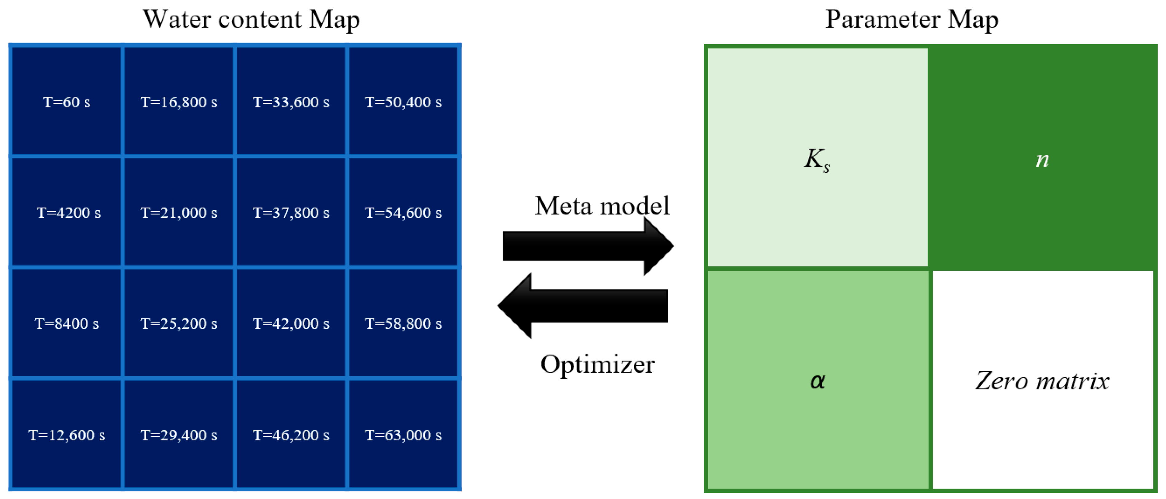
Latin hypercube sampling (LHS) was performed to generate samples from the k s ,   α , and n parameter spaces. These samples were then fed into the numerical model-based Monte Carlo simulation (MCS). For each combination of model inputs, the resulting model output soil moisture distributions at 16 different time steps were extracted and transformed to grayscale images (with a resolution of 8 × 8 pixels) by scaling moisture values between 0 and 255. These 16 images were then stacked together to create a single 32 × 32 pixel as shown in Figure 2. The use of 16 images allows for the characterization of the transient nature of soil moisture dynamics. To frame the problem as one of image-to-image regression, the input parameter values were also transformed into images by dividing a 32 × 32 pixel image (same size as the moisture images) into four equal blocks and assigning the scaled values (0,1) of each parameter to a block. This left us with one extra block which was always assigned a zero value. Hence, the training and validation datasets consisted of pairs of 32 × 32 pixel grayscale images. In this work, all images are displayed in colors to enhance the visual appeal. As an independent test dataset, a similar pair of 32 × 32 pixel grayscale input parameter–soil moisture images were also created from the laboratory experiment. In creating the input image, we neglected any heterogeneity in the input parameter distributions.

2.5. Model Training and Validation

The numerical model-based dataset was divided into three sub-sets consisting of 50, 30, and 20 percent of the image pairs for ED-CNN training, validation, and testing, respectively. The ED-CNN model construction and training were performed using Python Keras and TensorFlow libraries. The accuracy of the trained ED-CNN was assessed using three evaluation metrics, namely the coefficient of determination (R2 score), the Root mean squared error (RMSE), and the percentage error, calculated as follows [55,56]:
R M S E = 1 N i = 1 N y i y ^ i 2
R 2 = 1 i = 1 N y i y ^ i 2 i = 1 N y i m i 2
P e r c e n t a g e   e r r o r = T a r g e t   v a l u e P r e d i c t e d   v a l u e T a r g e t   v a l u e × 100
where y i and y ^ i represent the numerical model output and the ED-CNN predictions, respectively and m i denotes the mean value of the numerical model for N test data realizations.

3. Results and Discussion

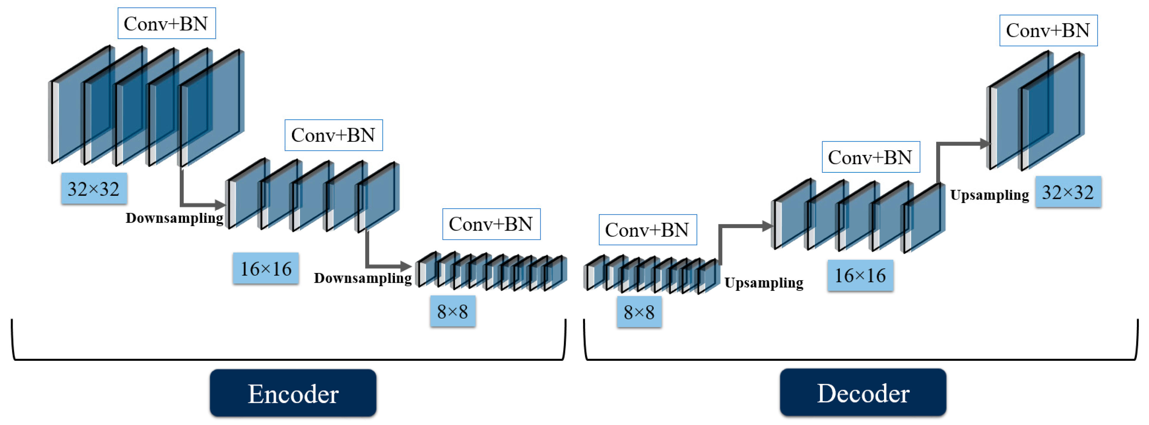
The proposed methodology was employed to develop: (1) an ED-CNN-based meta-model for soil moisture prediction, and (2) an ED-CNN-based optimizer to estimate k s , α , and n values from snapshots of the soil moisture during a drainage experiment. Based on trial and error, the ED-CNN architecture shown in Figure 3 and detailed in Table 2 was chosen for both meta-modeling and parameter estimation. The ED-CNN hyper-parameter values are presented in Table 3. The proposed network consists of 15 convolution layers, each of which is followed by a batch normalization layer. The kernel sizes for convolution and pooling layers are 3 × 3 and 2 × 2, respectively. The kernels are the same for all convolution and pooling layers.
All layers were activated using the rectified linear unit (ReLU) activation function, except the last three layers of the optimizer network, which used sigmoid for activation. The root mean squared propagation (RMSprop) and Adam optimizers were used for the meta-model and the optimizer networks, respectively. The mean squared error was selected as the loss function. ED-CNN training was performed on a PC with two Intel Xeon X5690 CPUs (3.4 GHz) (Intel Company, Santa Clara, CA, USA), which enabled the model to be trained in about 32 min for 150 epochs and 1000 training samples.

3.1. ED-CNN as Meta-Model

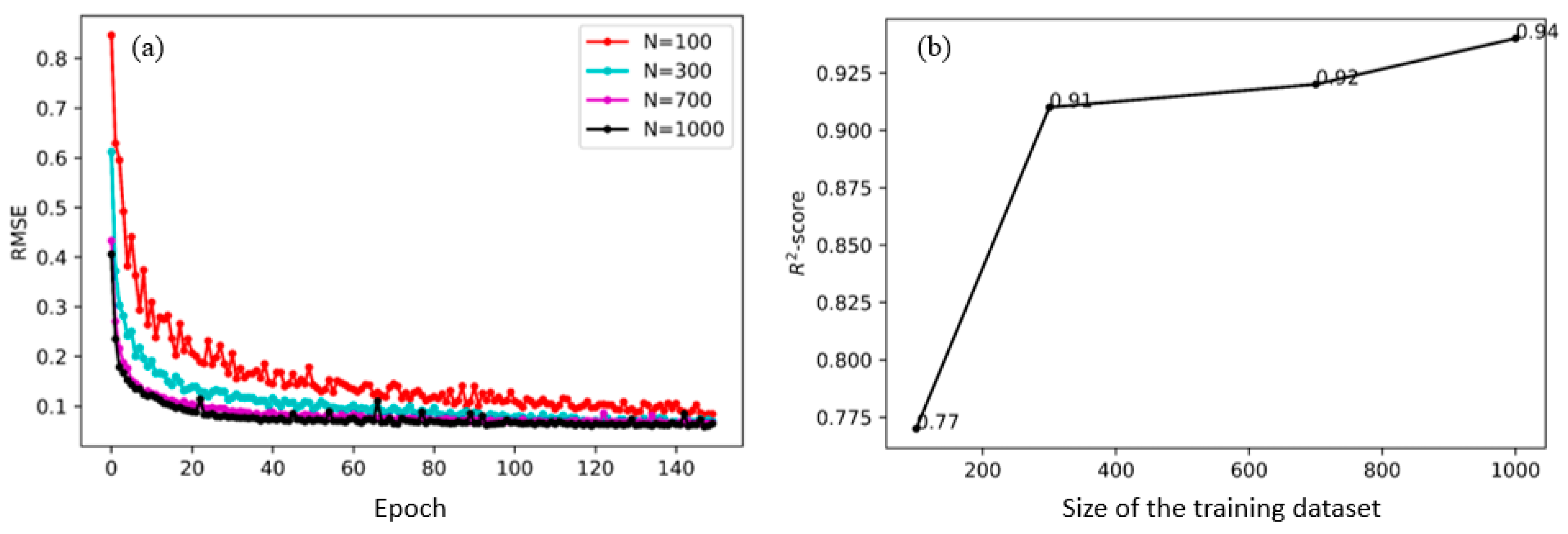
The performance of the ED-CNN for soil moisture prediction was assessed using both statistical criteria and visual inspection. The model was trained and evaluated using increasing numbers of training samples. As depicted in Figure 4a, when training the network using mean squared error loss, the RMSE training loss decreased sharply after just 20 epochs for all the assessed training sample sizes. For a training dataset consisting of 100 image pairs, the RMSE rapidly dropped to 0.2 after 20 epochs, whereas with 300 samples, the model achieved an RMSE of less than 0.1 after 20 epochs. As the number of epochs exceeded 20, the RMSE gradually converged to a constant value. As demonstrated, about 60 epochs were sufficient for ED-CNN meta-model training. Figure 4b shows R2 score variations with respect to the training sample size. This plot clearly shows that increasing the sample size from 100 to 300 improved the R2 score from 0.77 to 0.91, whereas using 700 or more samples only slightly increased the model accuracy.
Figure 5 shows an example of ED-CNN soil moisture predictions randomly chosen from the test dataset. To improve visual clarity, soil moisture images in 4 (out of the 16 predicted) time steps have been selected and visualized. The difference between numerical and ED-CNN results (i.e., the error) was calculated pixel by pixel, resulting in errors ranging between −0.04 cm3·cm−3 to 0.02 cm3·cm−3. As demonstrated, ED-CNN predictions (Figure 5b) show significant similarity with the numerical model output soil moisture distributions (Figure 5a) with low rates of error (Figure 5c).
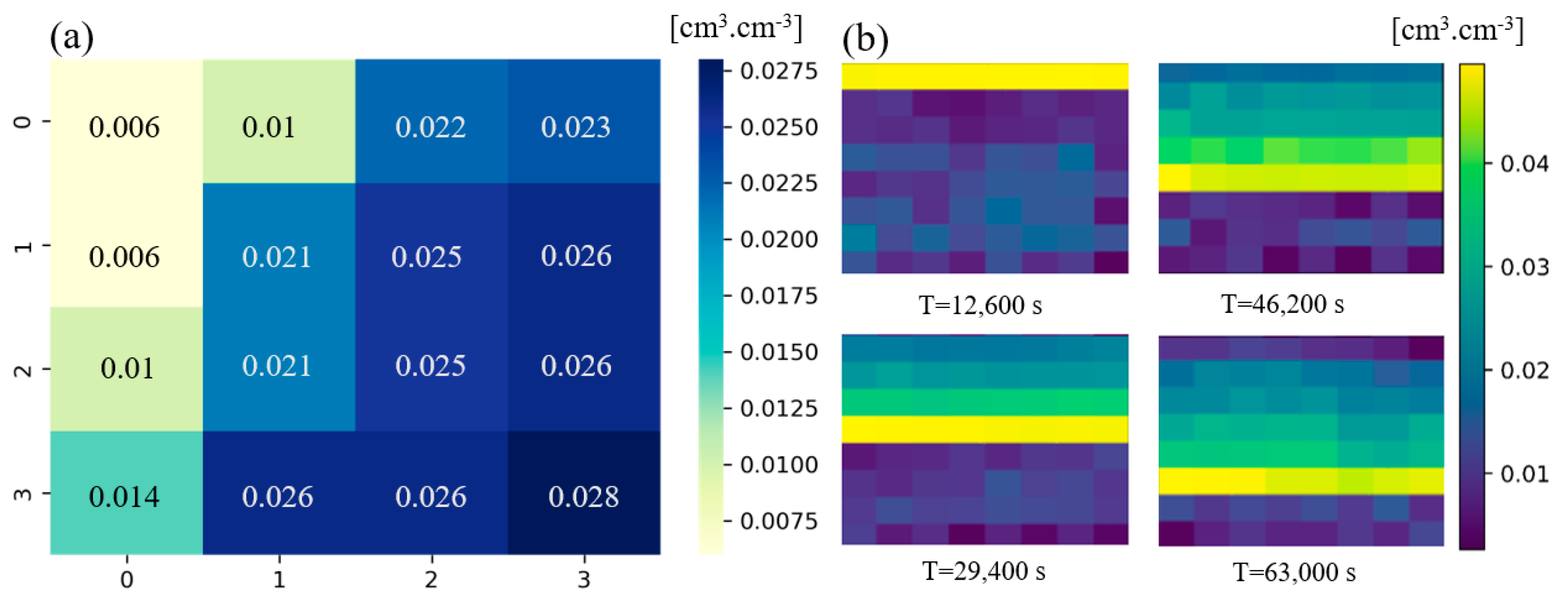
The RMSE averaged over each time step for 200 test cases was calculated and is illustrated in Figure 6a. This figure shows that the maximum average RMSE, equal to 0.028 cm3·cm−3, occurred at the last time step when the maximum drainage had been achieved. The spatial distribution of pixel-wise average RMSE for the 200 test cases in 4 time steps is depicted in Figure 6b. The figure shows that on average, the maximum error for each step occurred at the moving front of the saturation profile. To further assess the ED-CNN meta-model performance, the average RMSE histogram for the 200 test cases is presented in Figure 7. For the ED-CNN as a meta-model, the maximum value of the RMSE in a test sample was 0.079 cm3·cm−3, and 87% of the RMSEs were 0.023 cm3·cm−3. The distribution of the RMSE is close to a log-normal distribution skewed to the left.

3.2. ED-CNN for Uncertainty Analysis

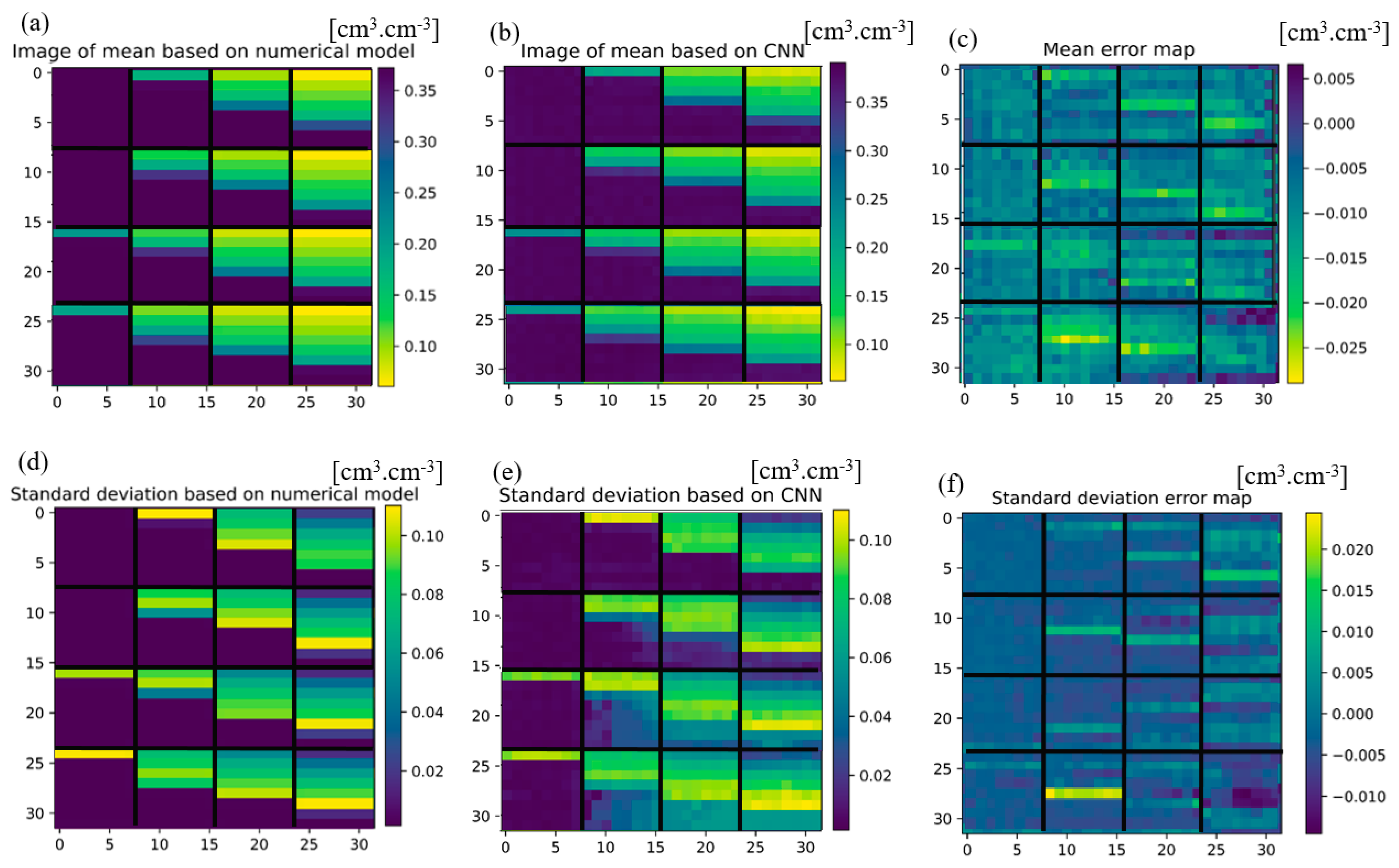
Commonly, the objective of using data-driven meta-models is not to provide single predictions but to facilitate tasks that require many simulations. This is most notably reflected in uncertainty propagation analysis (UPA). In this subsection, the effectiveness of ED-CNN in addressing the UPA of unsaturated flow predictions is evaluated. For this purpose, two MCSs were carried out, one based on the numerical model, and the other using the trained ED-CNN meta-model (see Section 3.1). Both MCSs were based on 1000 samples obtained through LHS. The outcomes of the MCSs were employed to compute the mean ( μ ) and the standard deviation ( σ ) of the soil moisture at different time steps. Figure 8 provides a comparison between the spatial distributions of μ and σ based on the numerical model and the ED-CNN. There is a high degree of similarity between Figure 8a,b for μ , and Figure 8d,e for σ , demonstrating the ability of the ED-CNN to replace the numerical model in Monte Carlo UPA of unsaturated flow simulations. Figure 8c,f demonstrate the pixel-by-pixel difference between the values of μ and σ generated from ED-CNN predictions and the numerical model. The difference for μ and σ varied between −0.028 to 0.0065 cm3·cm−3 and −0.014 to 0.0244 cm3·cm−3, respectively. The maximum error for both μ and σ occurred at the moving front of the saturation profile.
To investigate the computational efficiency gained by substituting the numerical model with ED-CNN, the time-saving ratio (TSR) is computed as follows [57]:
T S R = T N T m T N
where T N is the time required to perform calculations using the numerical model, and T m is the time needed to perform the same simulations using the meta-model. The latter encompasses both the time required for learning and the time taken for predictions by the neural network. The TSR for ED-CNN exceeds 0.989, showing a high rate of time saving for image-to-image regression of large input–output spaces.

3.3. ED-CNN as an Optimizer

3.3.1. Model Training and Validation Using Numerical Simulation Data

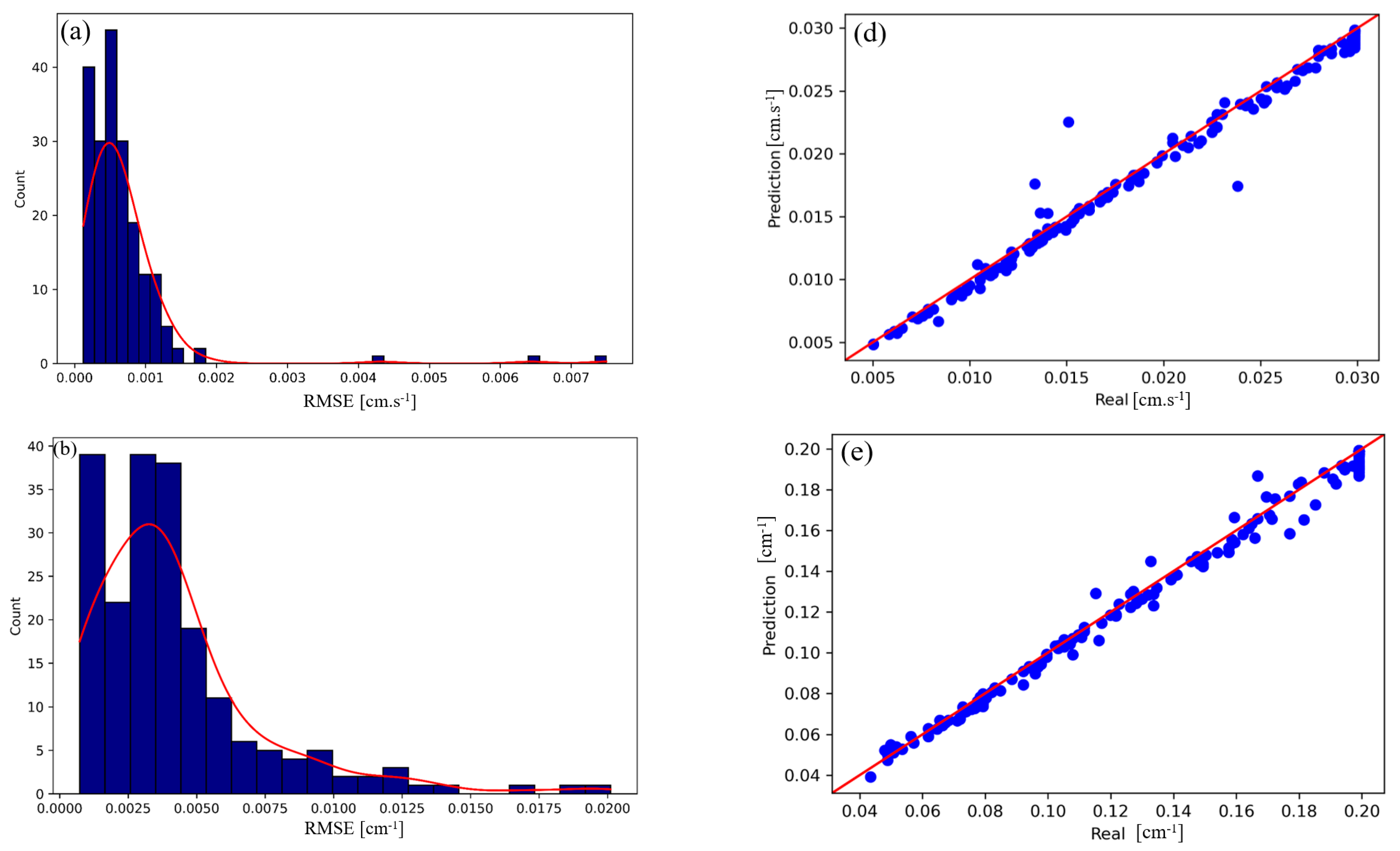
As explained in the methodology section, an independent ED-CNN model was trained for inverse modeling, using the stacked soil moisture images in 16 time steps (generated by the numerical model) as input, and the image describing   k s ,   α , and n values as output. We refer to this as the optimizer ED-CNN. The optimizer network was trained using the mean squared error loss function. Figure 9a demonstrates that, based on only 100 realizations and about 25 epochs, the optimizer’s overall RMSE training loss decreased to 0.1. It is also clear that after about 100 epochs, the RMSE converged to a constant value. This is also confirmed in Figure 9b, where the model R2 score reaches about 0.89 using 100 samples, whereas training the ED-CNN optimizer using more realizations does not significantly improve the accuracy. The RMSE histogram for ED-CNN as an optimizer is shown in Figure 10a–c. The maximum value of average RMSE for a test case for   k s is 0.0074 cm·s−1, while 94% of RMSE values do not exceed 0.001 cm·s−1. Maximum RMSE for α is 0.02 cm−1 but 82% of errors are less than 0.075 cm−1. The highest RMSE value for n is equal to 1.29 and 95% of errors for test samples are less than 0.4. For all parameters, the RMSE distribution is skewed to the left and resembles a log-normal distribution. Moreover, to better compare real and predicted values for each parameter, a scatter plot was calculated and is visualized in Figure 10d–f. It is evident from the results that there is significant agreement between real values and ED-CNN predictions. The percentage errors between real values for all 200 test cases and ED-CNN predictions for   k s ,   α , and n are about 0.3%, 1.4%, and 1%, which indicates that the ED-CNN architecture meets the accuracy requirements and hydraulic parameters can be precisely estimated using this method.

3.3.2. Comparison with Previous Studies

Table 4 compares the results of previous studies on unsaturated flow parameter estimation with those of the current study. These are past studies in which: (1) k s , α , and/or n are estimated, (2) the percentage error is provided so we have comparable metrics, and (3) the benchmark is numerical model simulation results as in the current study.
Prior research has primarily focused on employing 1D domains to estimate the parameters of the Richards equation, with the exception of a study by [12] which utilized a 2D model to estimate k s and α . Furthermore, these studies can be categorized into three groups. Ref. [58] utilized actual ground penetration radar data to estimate parameters, while [12,59,60] estimated parameters using hypothetical data. Finally, [61,62] incorporated a combination of real and hypothetical data in their studies.
These studies have employed a variety of techniques for parameter estimation, including ensemble Kalman filters, Gaussian processes, and analytical solutions. The percentage error in estimating k s in previous studies ranged from 1% to 20%, while the average percentage error in the ED-CNN estimates was 0.3%. Additionally, previous studies have estimated α and n with percentage errors ranging from 1–28% and 1–10%, respectively. The average percentage error in this study was 1.4% for α and 1% for n. Hence, the percentage errors of ED-CNN-based unsaturated flow parameter estimation in the current study are in the lower range of values from previous studies.

3.3.3. Parameter Estimation Using Photographic Imaging Data

Photographic imaging techniques enable mapping of the water content at fine resolution in 2D [53,63]), making them particularly appealing for the estimation of unsaturated flow parameters through ED-CNN-based image-to-image regression. To demonstrate this potential, we employed non-intrusive photographic images of a sandbox flow tank from [51] to estimate k s , α , and n . Figure 11 shows the ED-CNN input image created from stacking 16 photographic images of the sandbox flow tank obtained at the time steps described in Figure 2 and preprocessed according to Section 2.2 and Section 2.3. This image was fed into the trained ED-CNN optimizer and the resulting estimates of the unsaturated flow parameters are presented in Table 5. The target values of these parameters are also presented in Table 5. The percentage error for ED-CNN-based   k s , α , and n estimates were 5%, 13%, and 54%, respectively. Hence, the ED-CNN optimizer predicted two parameters (   k s and α ) with acceptable accuracy, while the predicted value of n was notably lower than the target value.

4. Conclusions

In this study, our main objectives were to assess the precision of ED-CNNs in predicting soil moisture distribution and to investigate their effectiveness as optimizers for inverse modeling in unsaturated flow simulations. By incorporating ED-CNNs and employing image-stacking techniques, we introduced novel approaches to forward and inverse modeling of water flow in unsaturated porous media. The study focused on theoretical development and utilized a simple problem involving a drainage experiment with a homogeneous sandbox flow tank packed with monodisperse quartz sand. The developed model was able to provide relatively accurate approximations with limited training samples, effectively tackling the high-dimensionality problem associated with image-to-image regression. This study relied on numerical model-based Monte Carlo simulation to generate data for ED-CNN training and validation. Furthermore, images obtained through non-intrusive photographic imaging were used for validation of the ED-CNN optimizer. The objective of the latter is to demonstrate that in addition to numerical model data, ED-CNN can also be used to handle image datasets obtained from high-resolution imaging and non-destructive scanning techniques that are becoming increasingly popular. Based on a drainage case study, we demonstrated that 60 epochs and 300 input–output realizations were sufficient to train an ED-CNN that achieved an R2 score of more than 91% for soil moisture predictions. For the ED-CNN optimizer, 100 epochs and 100 samples were required to train the model with an R2 score of more than 89%. In soil moisture predictions, the maximum average RMSE is seen at the last time step, when maximum drainage has been achieved. The spatial distribution of pixel-wise average RMSE shows that the maximum error for each time step occurred at the moving front of the saturation profile. Future work may consider applying the developed methodology to (a) heterogeneous porous media, (b) a complete drainage–imbibition cycle, and (c) modeling solute transport in unsaturated porous media.

Author Contributions

Conceptualization, M.M.R.; Methodology, M.M.R. and M.F.; Software, M.R.H.J. and M.F.; Validation, N.K.; Investigation, M.R.H.J. and N.K.; Data curation, B.B.; Writing—original draft, M.R.H.J. and M.M.R.; Writing—review & editing, M.F. and B.B.; Visualization, M.R.H.J.; Funding acquisition, M.F. All authors have read and agreed to the published version of the manuscript.

Funding

This research received funding form Strasbourg University and ENGEES for the experimental material and the APC.

Data Availability Statement

Not applicable.

Conflicts of Interest

The authors declare no conflict of interest.

References

  1. Farthing, M.W.; Ogden, F.L. Numerical solution of Richards’ equation: A review of advances and challenges. Soil Sci. Soc. Am. J. 2017, 81, 1257–1269. [Google Scholar] [CrossRef] [Green Version]
  2. Rajabi, M.M.; Belfort, B.; Lehmann, F.; Weill, S.; Ataie-Ashtiani, B.; Fahs, M. An improved Kalman filtering approach for the estimation of unsaturated flow parameters by assimilating photographic imaging data. J. Hydrol. 2020, 590, 125373. [Google Scholar] [CrossRef]
  3. Richards, L.A. Capillary Conduction of Liquids through Porous Mediums. Physics 1931, 1, 318–333. [Google Scholar] [CrossRef]
  4. Van Genuchten, M.T. A closed-form equation for predicting the hydraulic conductivity of unsaturated soils. Soil Sci. Soc. Am. J. 1980, 44, 892–898. [Google Scholar] [CrossRef] [Green Version]
  5. Sklorz, S.; Kaltofen, M.; Monninkhoff, B. Application of the FEFLOW groundwater model in the Zayandeh Rud catchment. In Reviving the Dying Giant: Integrated Water Resource Management in the Zayandeh Rud Catchment, Iran; Springer: Cham, Switzerland, 2017; pp. 241–251. [Google Scholar]
  6. Beegum, S.; Šimůnek, J.; Szymkiewicz, A.; Sudheer, K.; Nambi, I.M. Updating the Coupling Algorithm between HYDRUS and MODFLOW in the HYDRUS Package for MODFLOW. Vadose Zone J. 2018, 17, 1–8. [Google Scholar] [CrossRef] [Green Version]
  7. Dey, S.; Dhar, A. Generalized mass-conservative finite volume framework for unified saturated–unsaturated subsurface flow. J. Hydrol. 2022, 605, 127309. [Google Scholar] [CrossRef]
  8. Pollacco, J.; Fernández-Gálvez, J.; Ackerer, P.; Belfort, B.; Lassabatere, L.; Angulo-Jaramillo, R.; Rajanayaka, C.; Lilburne, L.; Carrick, S.; Peltzer, D. HyPix: 1D physically based hydrological model with novel adaptive time-stepping management and smoothing dynamic criterion for controlling Newton–Raphson step. Environ. Model. Softw. 2022, 153, 105386. [Google Scholar] [CrossRef]
  9. Li, C.; Ren, L. Estimation of unsaturated soil hydraulic parameters using the ensemble Kalman filter. Vadose Zone J. 2011, 10, 1205–1227. [Google Scholar] [CrossRef]
  10. Moret-Fernández, D.; Peña-Sancho, C.; Latorre, B.; Pueyo, Y.; López, M. Estimating the van Genuchten retention curve parameters of undisturbed soil from a single upward infiltration measurement. Soil Res. 2017, 55, 682–691. [Google Scholar] [CrossRef] [Green Version]
  11. Younes, A.; Fahs, M.; Ackerer, P. Modeling of flow and transport in saturated and unsaturated porous media. Water 2021, 13, 1088. [Google Scholar] [CrossRef]
  12. Liu, K.; Huang, G.; Jiang, Z.; Xu, X.; Xiong, Y.; Huang, Q.; Šimůnek, J. A gaussian process-based iterative Ensemble Kalman Filter for parameter estimation of unsaturated flow. J. Hydrol. 2020, 589, 125210. [Google Scholar] [CrossRef]
  13. Rajabi, M.M.; Ataie-Ashtiani, B.; Simmons, C.T. Polynomial chaos expansions for uncertainty propagation and moment independent sensitivity analysis of seawater intrusion simulations. J. Hydrol. 2015, 520, 101–122. [Google Scholar] [CrossRef]
  14. Zhang, J.; Man, J.; Lin, G.; Wu, L.; Zeng, L. Inverse modeling of hydrologic systems with adaptive multifidelity Markov chain Monte Carlo simulations. Water Resour. Res. 2018, 54, 4867–4886. [Google Scholar] [CrossRef]
  15. Zheng, Q.; Zhang, J.; Xu, W.; Wu, L.; Zeng, L. Adaptive multi-fidelit data assimilation for nonlinear subsurface flow problems. Water Resour. Res. 2019, 55, 203–217. [Google Scholar] [CrossRef] [Green Version]
  16. Gadd, C.; Xing, W.; Nezhad, M.M.; Shah, A. A surrogate modelling approach based on nonlinear dimension reduction for uncertainty quantification in groundwater flow models. Transp. Porous Media 2019, 126, 39–77. [Google Scholar] [CrossRef] [Green Version]
  17. Wu, B.; Zheng, Y.; Wu, X.; Tian, Y.; Han, F.; Liu, J.; Zheng, C. Optimizing water resources management in large river basins with integrated surface water-groundwater modeling: A surrogate-based approach. Water Resour. Res. 2015, 51, 2153–2173. [Google Scholar] [CrossRef]
  18. Zhu, P.; Shi, L.; Zhu, Y.; Zhang, Q.; Huang, K.; Williams, M. Data assimilation of soil water flow via ensemble Kalman filter: Infusing soil moisture data at different scales. J. Hydrol. 2017, 555, 912–925. [Google Scholar] [CrossRef] [Green Version]
  19. Mady, A.; Shein, E. Support vector machine and nonlinear regression methods for estimating saturated hydraulic conductivity. Mosc. Univ. Soil Sci. Bull. 2018, 73, 129–133. [Google Scholar] [CrossRef]
  20. Dwelle, M.C.; Kim, J.; Sargsyan, K.; Ivanov, V.Y. Streamflow, stomata, and soil pits: Sources of inference for complex models with fast, robust uncertainty quantification. Adv. Water Resour. 2019, 125, 13–31. [Google Scholar] [CrossRef]
  21. Wang, H.; Gong, W.; Duan, Q.; Di, Z. Evaluation of parameter interaction effect of hydrological models using the sparse polynomial chaos (SPC) method. Environ. Model. Softw. 2020, 125, 104612. [Google Scholar] [CrossRef]
  22. Tran, V.N.; Kim, J. A robust surrogate data assimilation approach to real-time forecasting using polynomial chaos expansion. J. Hydrol. 2021, 598, 126367. [Google Scholar] [CrossRef]
  23. Bandai, T.; Ghezzehei, T.A. Physics-informed neural networks with monotonicity constraints for Richardson-Richards equation: Estimation of constitutive relationships and soil water flux density from volumetric water content measurements. Water Resour. Res. 2021, 57, e2020WR027642. [Google Scholar] [CrossRef]
  24. Depina, I.; Jain, S.; Mar Valsson, S.; Gotovac, H. Application of physics-informed neural networks to inverse problems in unsaturated groundwater flow. Georisk: Assess. Manag. Risk Eng. Syst. Geohazards 2022, 16, 21–36. [Google Scholar] [CrossRef]
  25. Chai, Y.; Liu, H.; Yu, Y.; Yang, Q.; Zhang, X.; Zhao, W.; Guo, L.; Yetemen, O. Strategies of Parameter Optimization and Soil Moisture Sensor Deployment for Accurate Estimation of Evapotranspiration Through a Data-driven Method. Agric. For. Meteorol. 2023, 331, 109354. [Google Scholar] [CrossRef]
  26. Shuku, T.; Phoon, K.-K. Data-driven subsurface modelling using a Markov random field model. Georisk Assess. Manag. Risk Eng. Syst. Geohazards 2023, 17, 41–63. [Google Scholar] [CrossRef]
  27. Lyu, B.; Hu, Y.; Wang, Y. Data-driven development of three-dimensional subsurface models from sparse measurements using Bayesian compressive sampling: A benchmarking study. ASCE-ASME J. Risk Uncertain. Eng. Syst. Part A Civ. Eng. 2023, 9, 04023010. [Google Scholar] [CrossRef]
  28. Vu, M.; Jardani, A. Mapping of hydraulic transmissivity field from inversion of tracer test data using convolutional neural networks. CNN-2T. J. Hydrol. 2022, 606, 127443. [Google Scholar] [CrossRef]
  29. Asher, M.J.; Croke, B.F.; Jakeman, A.J.; Peeters, L.J. A review of surrogate models and their application to groundwater modeling. Water Resour. Res. 2015, 51, 5957–5973. [Google Scholar] [CrossRef] [Green Version]
  30. Mo, S.; Zhu, Y.; Zabaras, N.; Shi, X.; Wu, J. Deep convolutional encoder-decoder networks for uncertainty quantification of dynamic multiphase flow in heterogeneous media. Water Resour. Res. 2019, 55, 703–728. [Google Scholar] [CrossRef] [Green Version]
  31. Samek, W.; Montavon, G.; Lapuschkin, S.; Anders, C.J.; Müller, K.-R. Explaining deep neural networks and beyond: A review of methods and applications. Proc. IEEE 2021, 109, 247–278. [Google Scholar] [CrossRef]
  32. Tartakovsky, A.M.; Marrero, C.O.; Perdikaris, P.; Tartakovsky, G.D.; Barajas-Solano, D. Physics-informed deep neural networks for learning parameters and constitutive relationships in subsurface flow problems. Water Resour. Res. 2020, 56, e2019WR026731. [Google Scholar] [CrossRef]
  33. Stepanov, S.; Spiridonov, D.; Mai, T. Prediction of numerical homogenization using deep learning for the Richards equation. J. Comput. Appl. Math. 2023, 424, 114980. [Google Scholar] [CrossRef]
  34. Song, W.; Shi, L.; Hu, X.; Wang, Y.; Wang, L. Reconstructing the Unsaturated Flow Equation from Sparse and Noisy Data: Leveraging the Synergy of Group Sparsity and Physics-Informed Deep Learning. Water Resour. Res. 2023, 59, e2022WR034122. [Google Scholar] [CrossRef]
  35. Haruzi, P.; Moreno, Z. Modeling water flow and solute transport in unsaturated soils using physics-informed neural networks trained with geoelectrical data. Water Resour. Res. 2023, 59, e2023WR034538. [Google Scholar] [CrossRef]
  36. Zhu, Y.; Zabaras, N. Bayesian deep convolutional encoder–decoder networks for surrogate modeling and uncertainty quantification. J. Comput. Phys. 2018, 366, 415–447. [Google Scholar] [CrossRef] [Green Version]
  37. Zhang, H.; Yu, H.; Yuan, X.; Xu, H.; Micheal, M.; Zhang, J.; Shu, H.; Wang, G.; Wu, H. Permeability prediction of low-resolution porous media images using autoencoder-based convolutional neural network. J. Pet. Sci. Eng. 2022, 208, 109589. [Google Scholar] [CrossRef]
  38. Taccari, M.L.; Nuttall, J.; Chen, X.; Wang, H.; Minnema, B.; Jimack, P.K. Attention U-Net as a surrogate model for groundwater prediction. Adv. Water Resour. 2022, 163, 104169. [Google Scholar] [CrossRef]
  39. Davis, K.; Leiteritz, R.; Pflüger, D.; Schulte, M. Deep learning based surrogate modeling for thermal plume prediction of groundwater heat pumps. arXiv 2023, arXiv:2302.08199. [Google Scholar]
  40. Rajabi, M.M.; Javaran, M.R.H.; Bah, A.-o.; Frey, G.; Le Ber, F.; Lehmann, F.; Fahs, M. Analyzing the efficiency and robustness of deep convolutional neural networks for modeling natural convection in heterogeneous porous media. Int. J. Heat Mass Transf. 2022, 183, 122131. [Google Scholar] [CrossRef]
  41. Wen, G.; Tang, M.; Benson, S.M. Towards a predictor for CO2 plume migration using deep neural networks. Int. J. Greenh. Gas Control 2021, 105, 103223. [Google Scholar] [CrossRef]
  42. Jiang, Z.; Tahmasebi, P.; Mao, Z. Deep residual U-net convolution neural networks with autoregressive strategy for fluid flow predictions in large-scale geosystems. Adv. Water Resour. 2021, 150, 103878. [Google Scholar] [CrossRef]
  43. Wang, N.; Chang, H.; Zhang, D. Theory-guided auto-encoder for surrogate construction and inverse modeling. Comput. Methods Appl. Mech. Eng. 2021, 385, 114037. [Google Scholar] [CrossRef]
  44. Conway, A.M.; Durbach, I.N.; McInnes, A.; Harris, R.N. Frame-by-frame annotation of video recordings using deep neural networks. Ecosphere 2021, 12, e03384. [Google Scholar] [CrossRef]
  45. Kong, Z.; Zhang, C.; Lv, H.; Xiong, F.; Fu, Z. Multimodal feature extraction and fusion deep neural networks for short-term load forecasting. IEEE Access 2020, 8, 185373–185383. [Google Scholar] [CrossRef]
  46. Bazai, H.; Kargar, E.; Mehrabi, M. Using an encoder-decoder convolutional neural network to predict the solid holdup patterns in a pseudo-2d fluidized bed. Chem. Eng. Sci. 2021, 246, 116886. [Google Scholar] [CrossRef]
  47. Zaccone, G.; Karim, M.R. Deep Learning with TensorFlow: Explore Neural Networks and Build Intelligent Systems with Python; Packt Publishing Ltd.: Birmingham, UK, 2018. [Google Scholar]
  48. Badrinarayanan, V.; Kendall, A.; Cipolla, R. Segnet: A deep convolutional encoder-decoder architecture for image segmentation. IEEE Trans. Pattern Anal. Mach. Intell. 2017, 39, 2481–2495. [Google Scholar] [CrossRef]
  49. Jardani, A.; Vu, T.; Fischer, P. Use of convolutional neural networks with encoder-decoder structure for predicting the inverse operator in hydraulic tomography. J. Hydrol. 2022, 604, 127233. [Google Scholar] [CrossRef]
  50. Xia, X.; Jiang, S.; Zhou, N.; Cui, J.; Li, X. Groundwater contamination source identification and high-dimensional parameter inversion using residual dense convolutional neural network. J. Hydrol. 2023, 617, 129013. [Google Scholar] [CrossRef]
  51. Belfort, B.; Weill, S.; Fahs, M.; Lehmann, F. Laboratory experiments of drainage, imbibition and infiltration under artificial rainfall characterized by image analysis method and numerical simulations. Water 2019, 11, 2232. [Google Scholar] [CrossRef] [Green Version]
  52. Mualem, Y. A new model for predicting the hydraulic conductivity of unsaturated porous media. Water Resour. Res. 1976, 12, 513–522. [Google Scholar] [CrossRef] [Green Version]
  53. Belfort, B.; Weill, S.; Lehmann, F. Image analysis method for the measurement of water saturation in a two-dimensional experimental flow tank. J. Hydrol. 2017, 550, 343–354. [Google Scholar] [CrossRef] [Green Version]
  54. Fahs, M.; Younes, A.; Lehmann, F. An easy and efficient combination of the Mixed Finite Element Method and the Method of Lines for the resolution of Richards’ Equation. Environ. Model. Softw. 2009, 24, 1122–1126. [Google Scholar] [CrossRef]
  55. Kumar, D.; Roshni, T.; Singh, A.; Jha, M.K.; Samui, P. Predicting groundwater depth fluctuations using deep learning, extreme learning machine and Gaussian process: A comparative study. Earth Sci. Inform. 2020, 13, 1237–1250. [Google Scholar] [CrossRef]
  56. Wang, N.; Chang, H.; Zhang, D. Surrogate and inverse modeling for two-phase flow in porous media via theory-guided convolutional neural network. J. Comput. Phys. 2022, 466, 111419. [Google Scholar] [CrossRef]
  57. Rajabi, M.M.; Ketabchi, H. Uncertainty-based simulation-optimization using Gaussian process emulation: Application to coastal groundwater management. J. Hydrol. 2017, 555, 518–534. [Google Scholar] [CrossRef]
  58. Tran, A.P.; Vanclooster, M.; Zupanski, M.; Lambot, S. Joint estimation of soil moisture profile and hydraulic parameters by ground-penetrating radar data assimilation with maximum likelihood ensemble filter. Water Resour. Res. 2014, 50, 3131–3146. [Google Scholar] [CrossRef]
  59. Shi, L.; Song, X.; Tong, J.; Zhu, Y.; Zhang, Q. Impacts of different types of measurements on estimating unsaturated flow parameters. J. Hydrol. 2015, 524, 549–561. [Google Scholar] [CrossRef]
  60. Hayek, M. Analytical solution to transient Richards’ equation with realistic water profiles for vertical infiltration and parameter estimation. Water Resour. Res. 2016, 52, 4438–4457. [Google Scholar] [CrossRef] [Green Version]
  61. Rai, P.K.; Tripathi, S. Gaussian process for estimating parameters of partial differential equations and its application to the Richards equation. Stoch. Environ. Res. Risk Assess. 2019, 33, 1629–1649. [Google Scholar] [CrossRef]
  62. Su, L.; Hou, L.; Zhou, B.; Shan, Y.; Duan, M.; Sun, Y.; Ning, S.; Wang, Q. Approximate analytical solution and parameter estimation for one-dimensional horizontal absorption based on the van Genuchten–Mualem model. Soil Sci. Soc. Am. J. 2021, 85, 217–234. [Google Scholar] [CrossRef]
  63. Yoshimoto, N.; Orense, R.P.; Tanabe, F.; Kikkawa, N.; Hyodo, M.; Nakata, Y. Measurement of degree of saturation on model ground by digital image processing. Soils Found. 2011, 51, 167–177. [Google Scholar] [CrossRef] [Green Version]
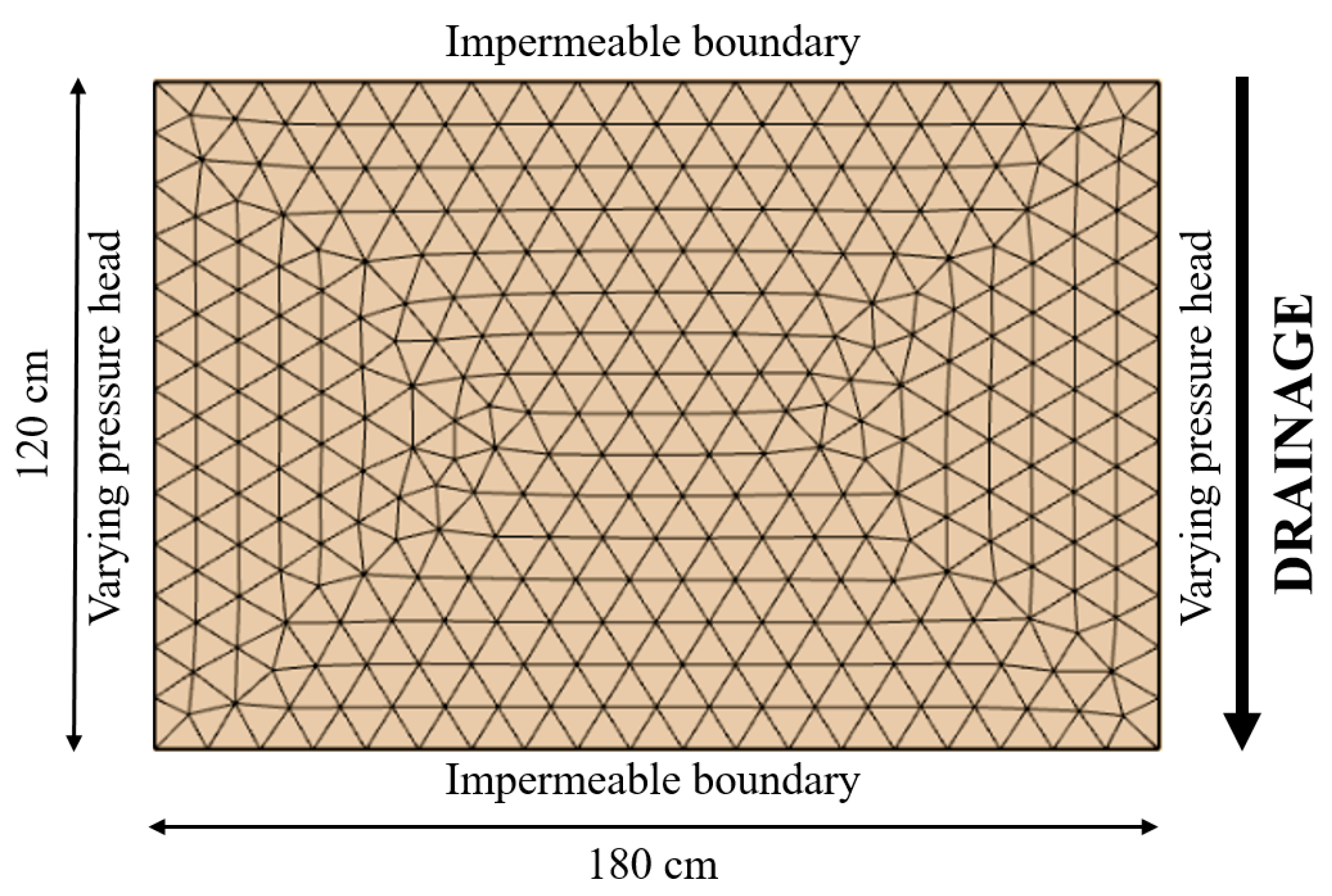
Figure 1. Conceptual model of the test case and its numerical grid.
Water 15 02890 g001
Figure 2. Schematic of input–output image pairs.
Water 15 02890 g002
Figure 3. Schematic of proposed ED-CNN architecture (Conv: convolution layer, BN: batch normalization layer).
Water 15 02890 g003
Figure 4. (a) RMSE as a function of epochs and (b) R 2 score as a function of the training dataset size of the proposed ED-CNN meta-model for soil moisture predictions.
Water 15 02890 g004
Figure 5. (a) Numerical model-based, and (b) ED-CNN-based soil moisture distribution in four time steps, in addition to (c) the resulting spatial distribution of the absolute difference between numerical and ED-CNN results.
Water 15 02890 g005
Figure 6. ED-CNN RMSE, averaged over each: (a) time step, and (b) pixel, for 200 test cases.
Water 15 02890 g006
Figure 7. ED-CNN RMSE histogram for 200 test cases.
Water 15 02890 g007
Figure 8. Spatial distribution of Monte Carlo- (ac) mean and (df) standard deviation estimations based on the numerical model and ED-CNN, and their associated differences.
Water 15 02890 g008
Figure 9. (a) RMSE and (b) R 2 score of the proposed ED-CNN optimizer for soil moisture predictions.
Water 15 02890 g009
Figure 10. (ac) RMSE histograms of k s , α , and n , respectively, and (df) scatter plots of target vs. predicted values of k s , α , and n , respectively, estimated by the ED-CNN. Plots are based on 200 realizations.
Water 15 02890 g010aWater 15 02890 g010b
Figure 11. Input image for the ED-CNN optimizer constructed from the photographic images of a sandbox flow tank in Belfort [51].
Water 15 02890 g011
Table 1. Characteristics of the hypothetical probability distribution functions (PDFs) for the uncertain input parameters.
ParameterPDFIntervalUnit
  k s [0.001, 0.03][cm·s−1]
α Uniform[0.001, 0.2][cm−1]
n [2, 8][-]
Table 2. The ED-CNN architecture details.
LayerKernel SizeResolution
Encoder
Convolution + Batch normalization3 × 332 × 32
Downsampling12 × 216 × 16
Convolution + Batch normalization3 × 316 × 16
Downsampling22 × 28 × 8
Convolution + Batch normalization3 × 38 × 8
Decoder
Convolution + Batch normalization3 × 38 × 8
Upsampling12 × 216 × 16
Convolution + Batch normalization3 × 316 × 16
Upsampling22 × 232 × 32
Convolution + Batch normalization3 × 332 × 32
Table 3. ED-CNN hyper-parameters details.
Hyper-ParameterMeta-ModelOptimizer
OptimizerRMSpropAdam
Loss functionMean squared errorMean squared error
Samples10001000
Test set200200
Validation set300300
Batch size1224
Epochs150300
Learning rate0.00010.0001
Table 4. Comparison of the results of previous studies on unsaturated flow parameter estimation with those of the current study.
ReferenceParameter Estimation MethodEstimated Hydraulic ParametersPercentage Error (%)
  k s α n
[58] EnKF   k s ,   α ,   n 3.23.61
[59]EnKF   k s 20--
[60]Analytical solution   k s ,   n 10-10
[61]GPPDE   k s ,   n 3.3-8.93
[12]EnKF   k s ,   α 11-
[62]Analytical solution α ,   n -3.2 to 280.4 to 8
Current optimizer studyED-CNN   k s ,   α ,   n 0.31.41
Note: EnKF: ensemble Kalman filter, GPPDE: Gaussian process for partial differential equation.
Table 5. Comparison between ED-CNN estimation using experiment images and the numerical model with real values.
ParameterExperiment Moisture Map as InputTarget Value
  k s 0.350.37
α 0.370.43
n 0.450.99
Note: all parameter values are normalized between (0, 1).
Disclaimer/Publisher’s Note: The statements, opinions and data contained in all publications are solely those of the individual author(s) and contributor(s) and not of MDPI and/or the editor(s). MDPI and/or the editor(s) disclaim responsibility for any injury to people or property resulting from any ideas, methods, instructions or products referred to in the content.