


The Investigation of Local Scour around Bridge Piers with the Protection of a Quasi-Stumps Group


Abstract
:1. Introduction
2. Materials and Methods
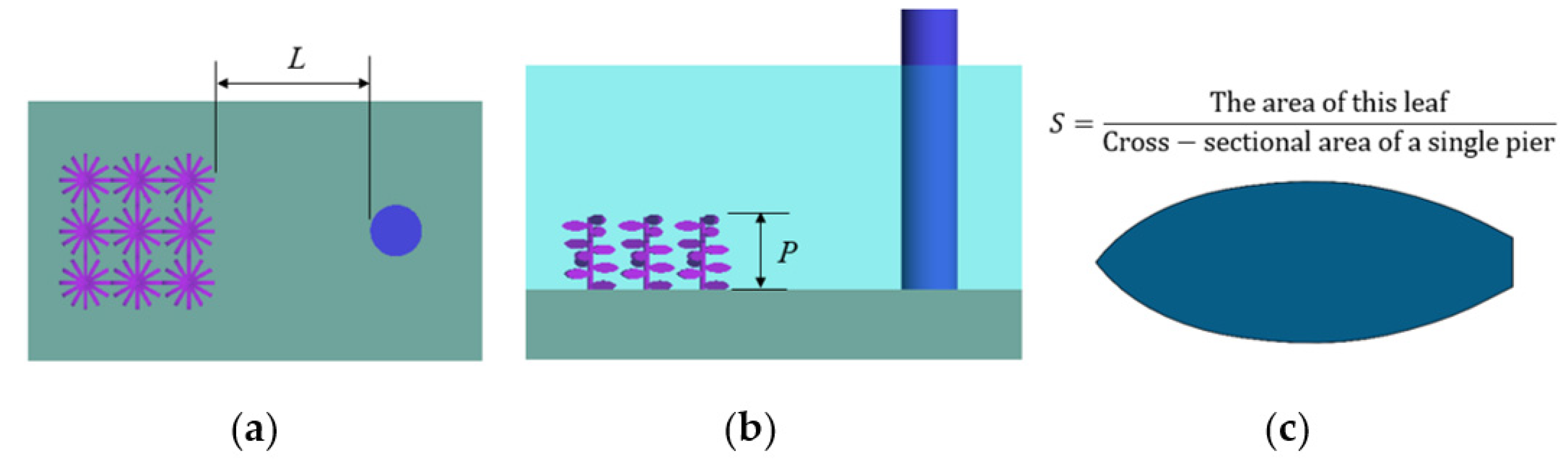
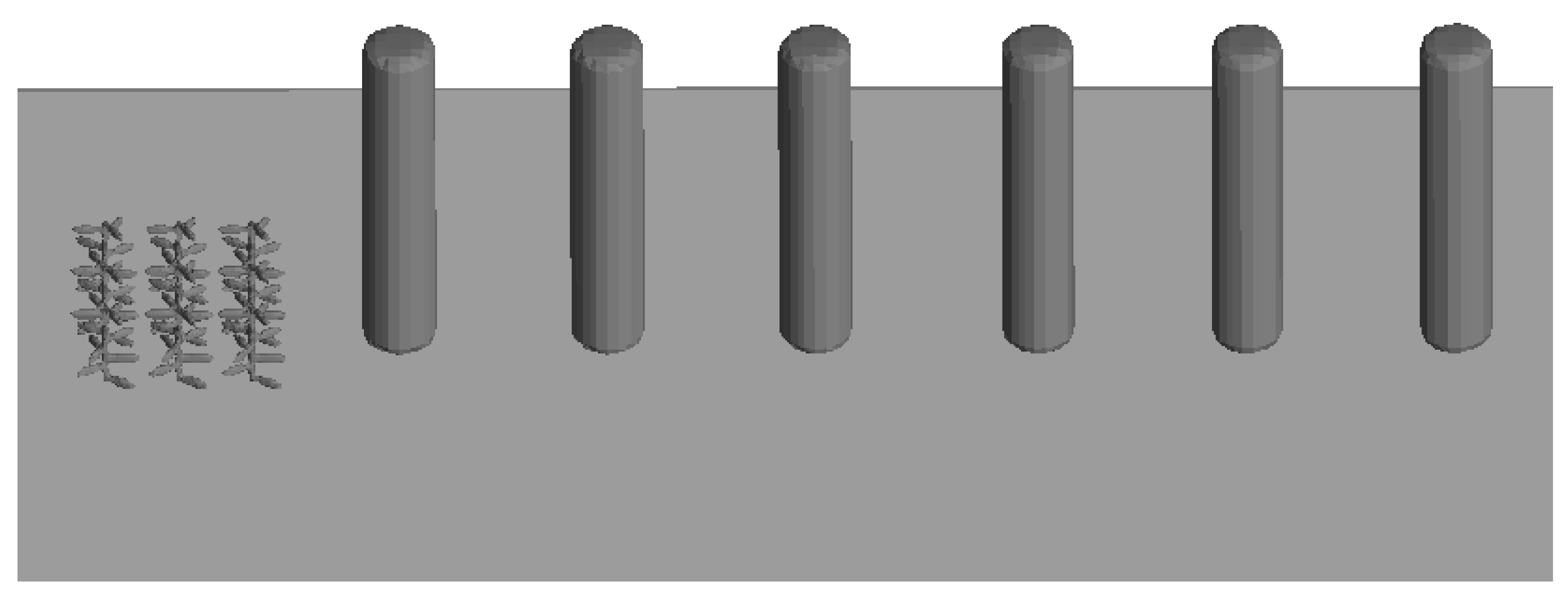
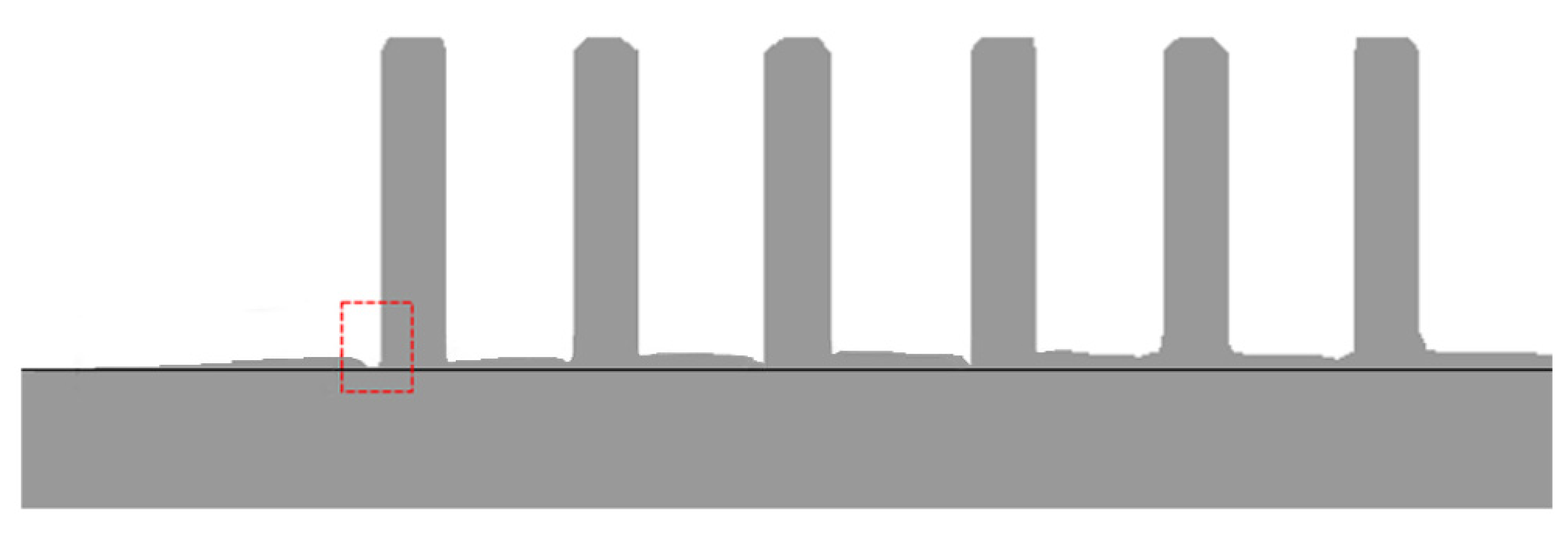
2.1. Structure of Quasi-Stumps Group
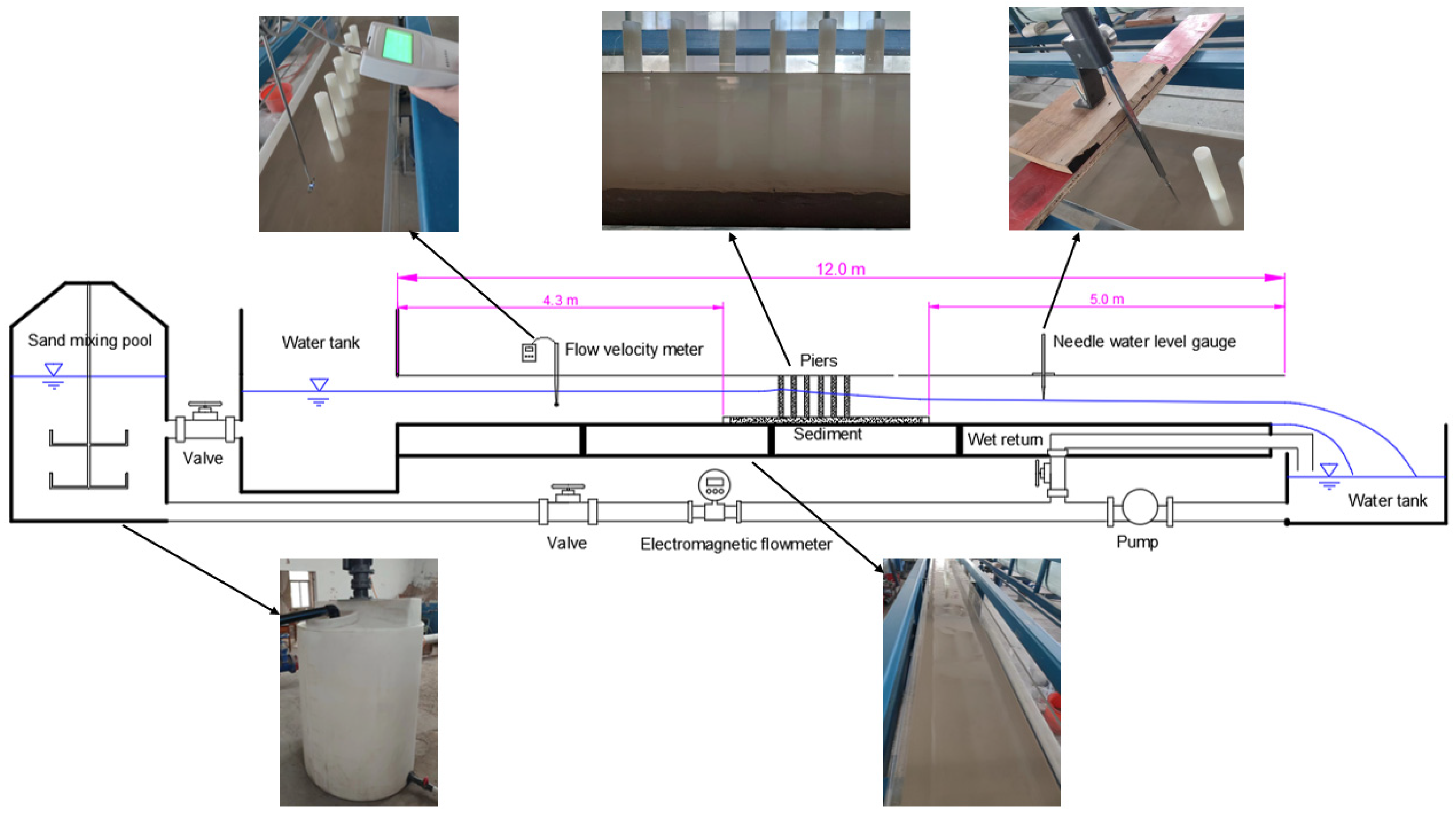
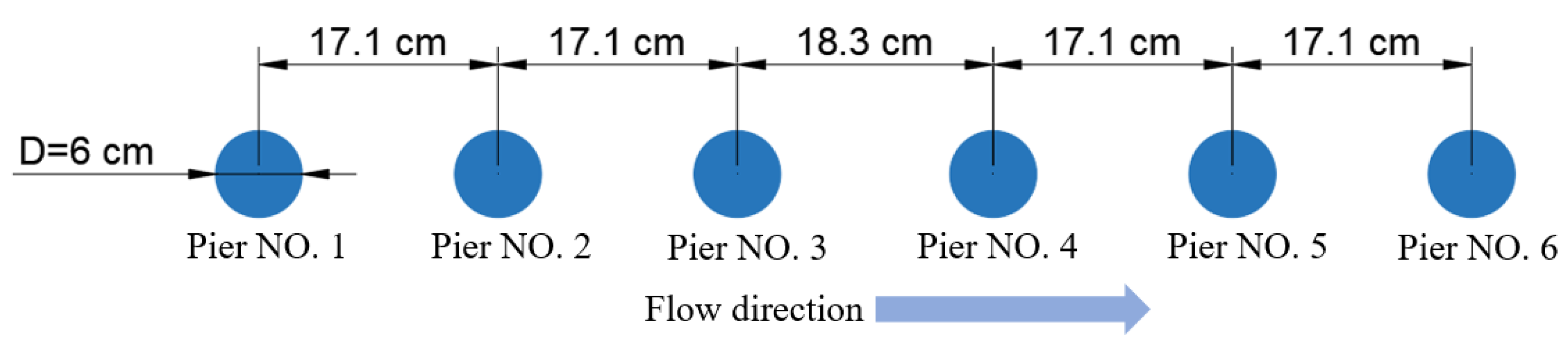
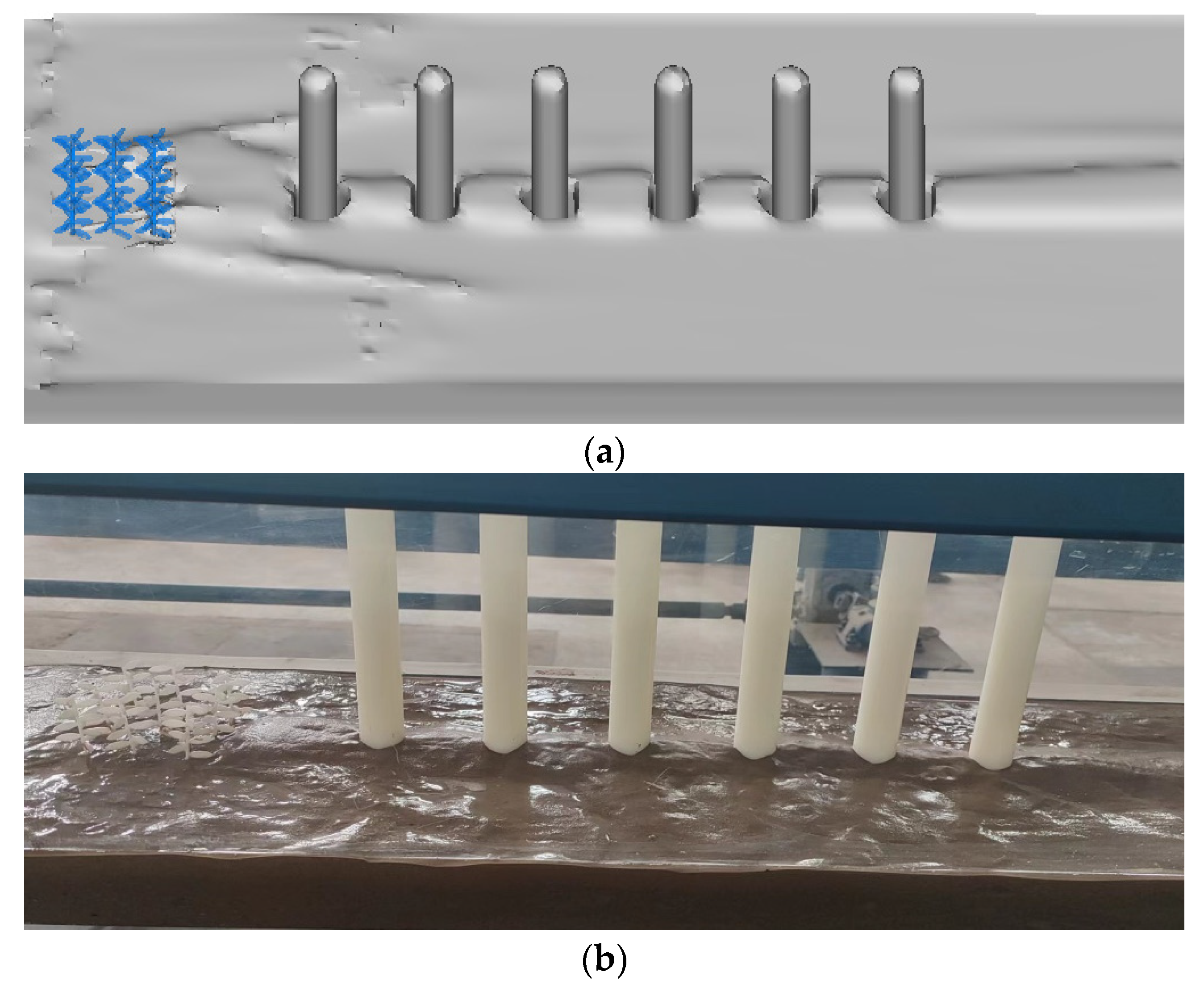
2.2. Experimental Setup
2.3. Numerical Simulation
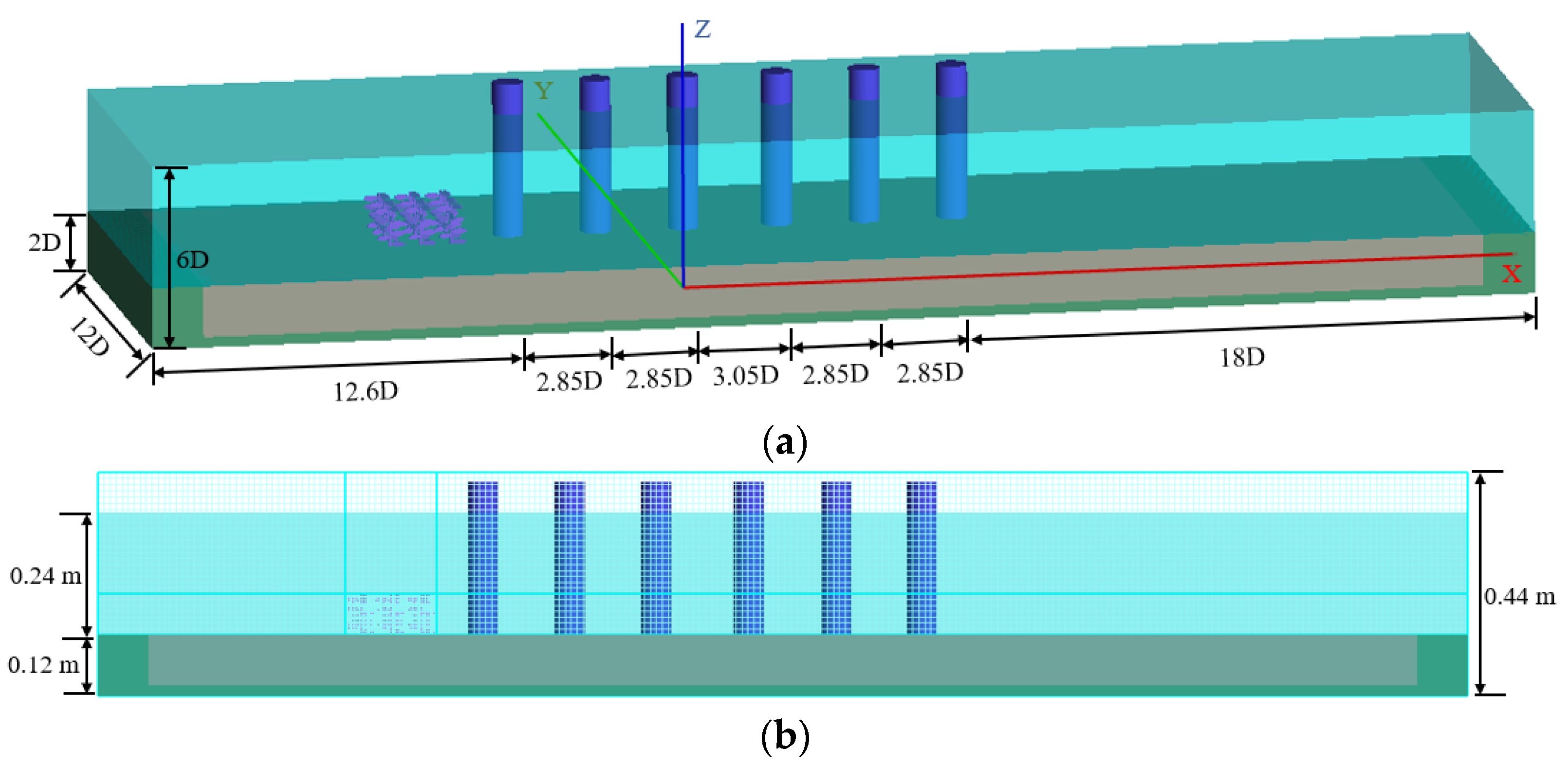
2.4. Computational Domain
2.5. Experimental Variables and Working Conditions
2.6. Grid and User-Defined Parameters
3. Results
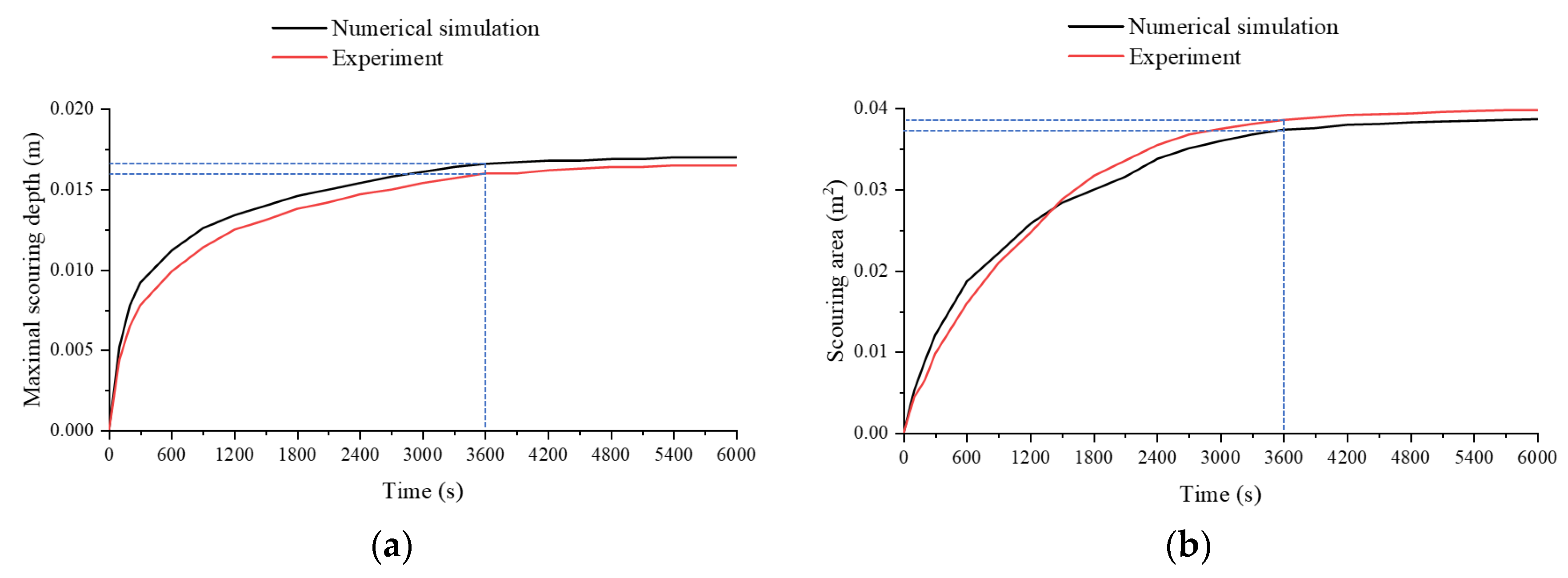
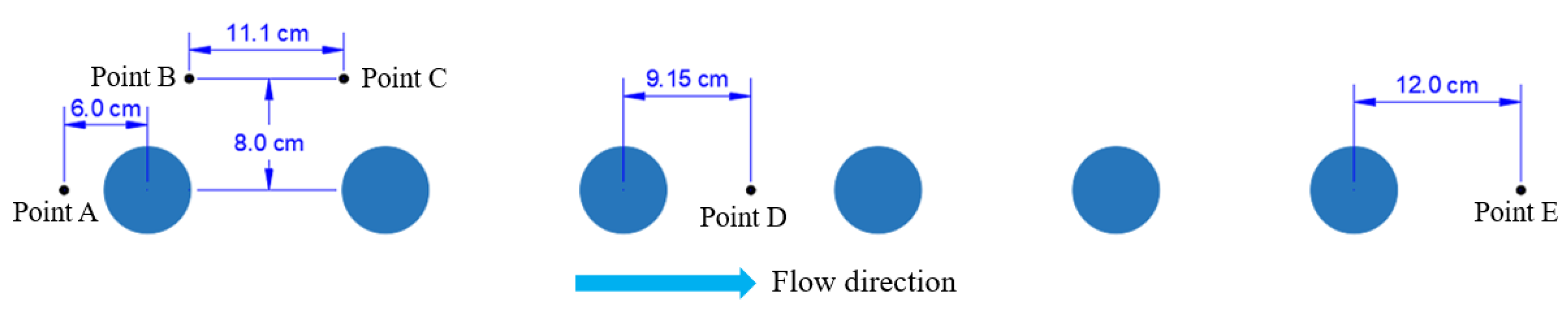
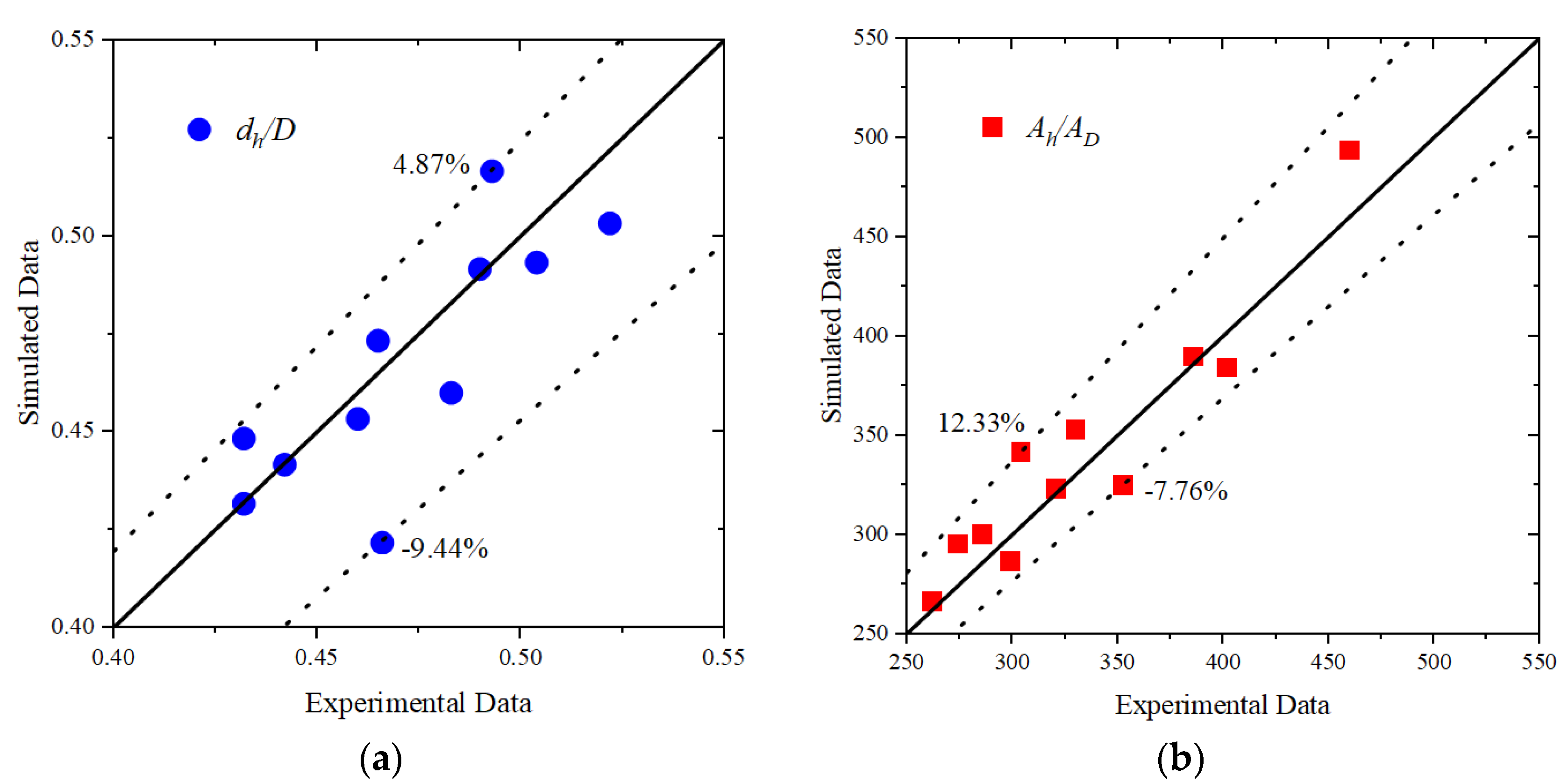
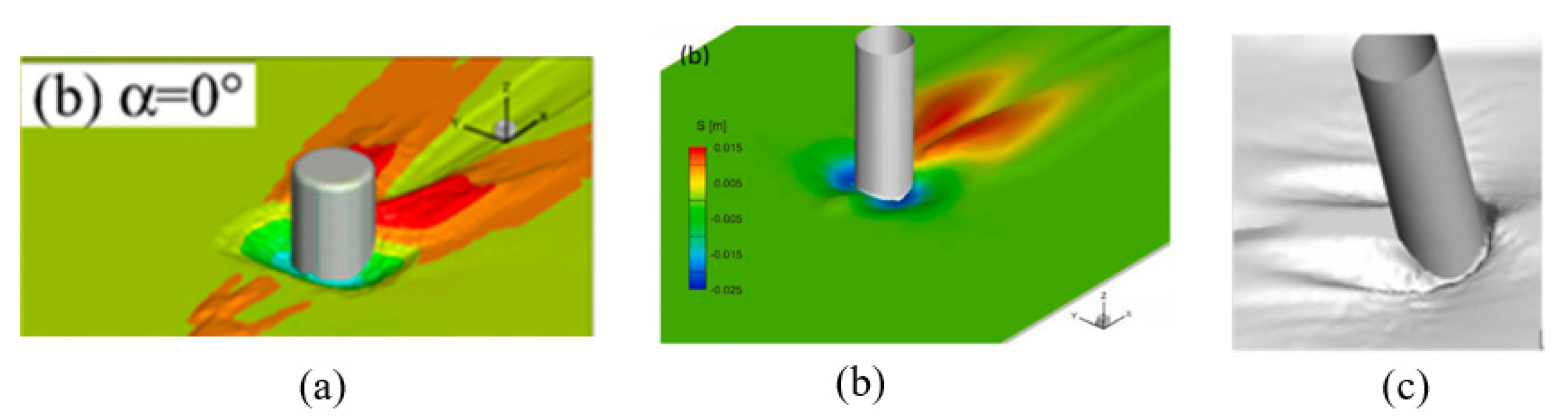
3.1. Validation
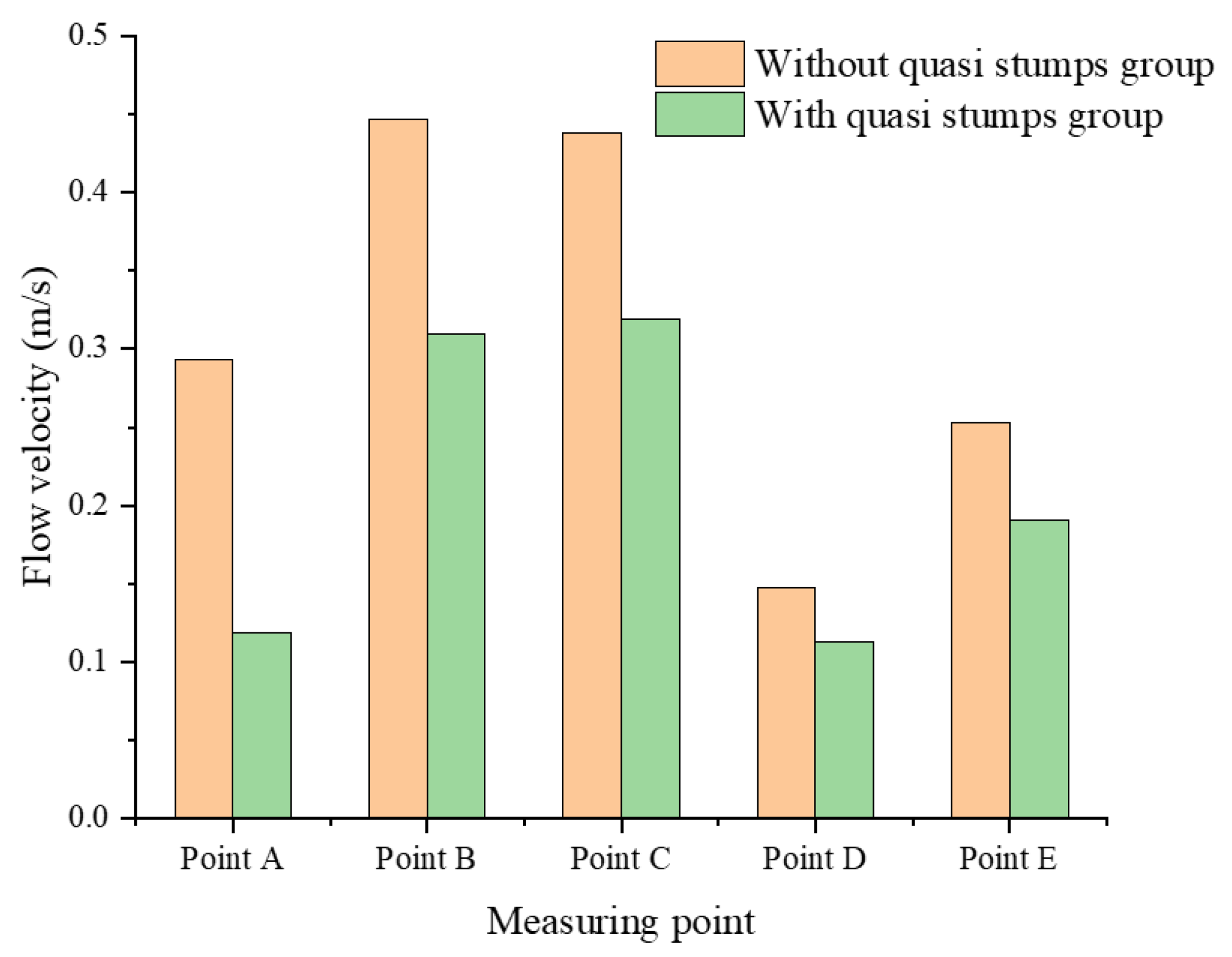
3.2. Protective Effect of the Quasi-Stumps Group
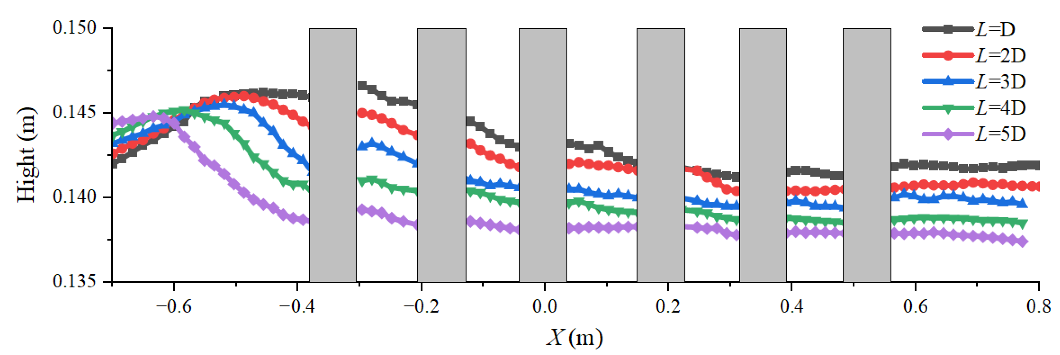
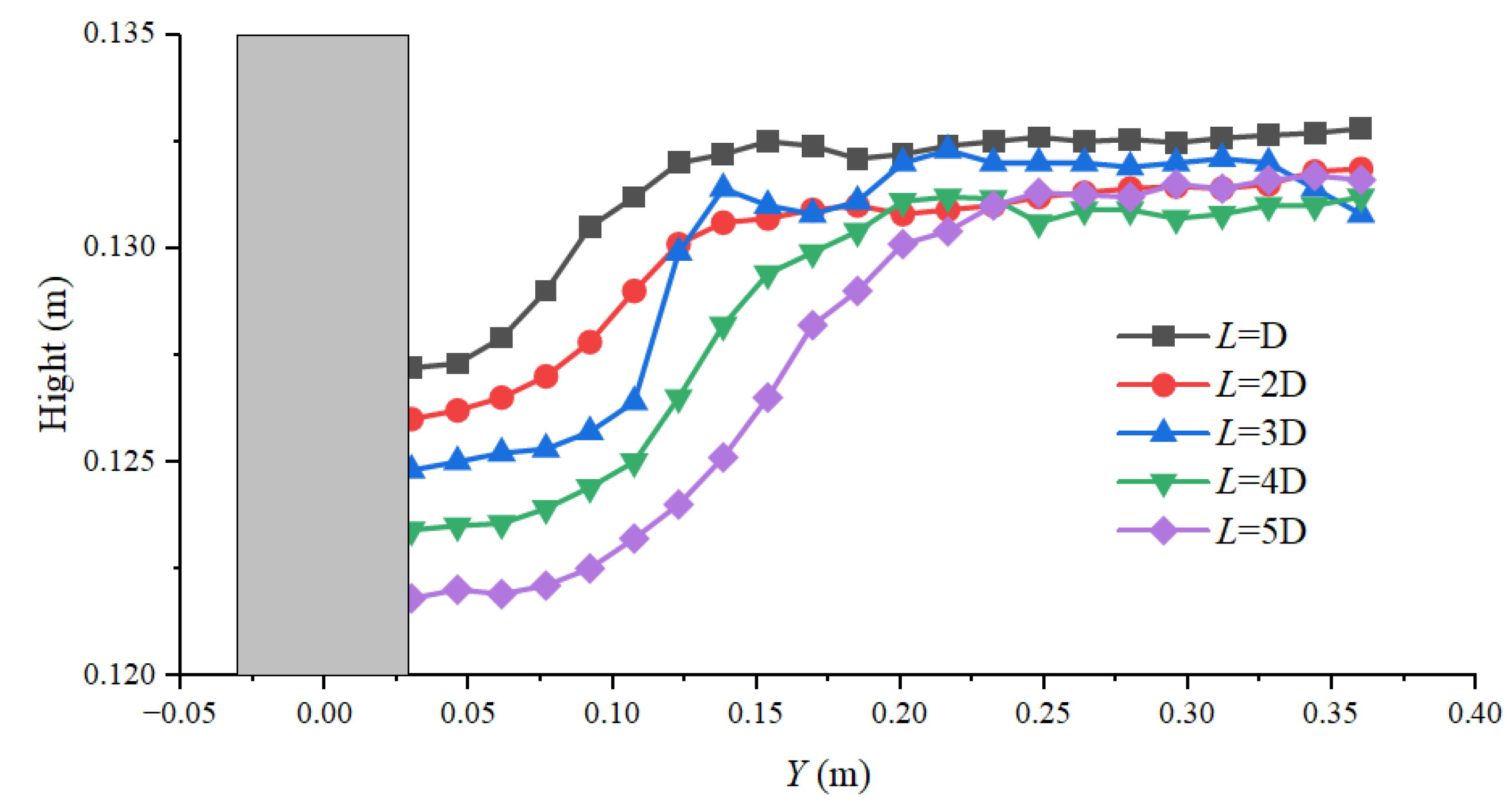
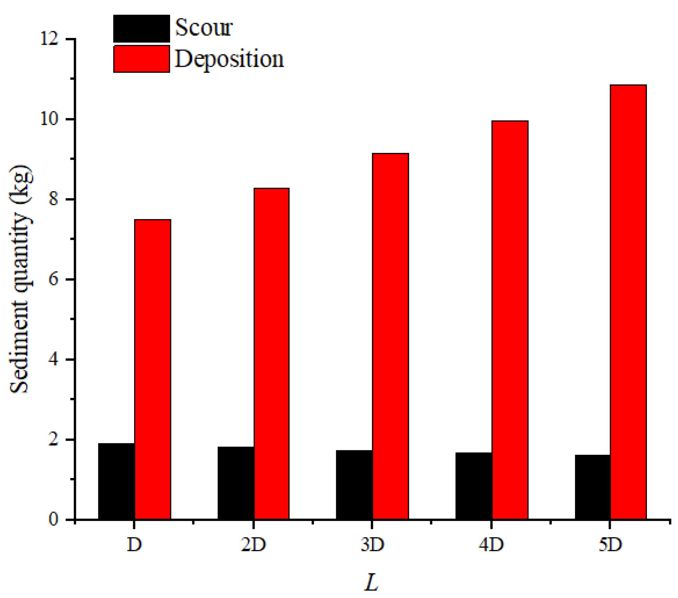
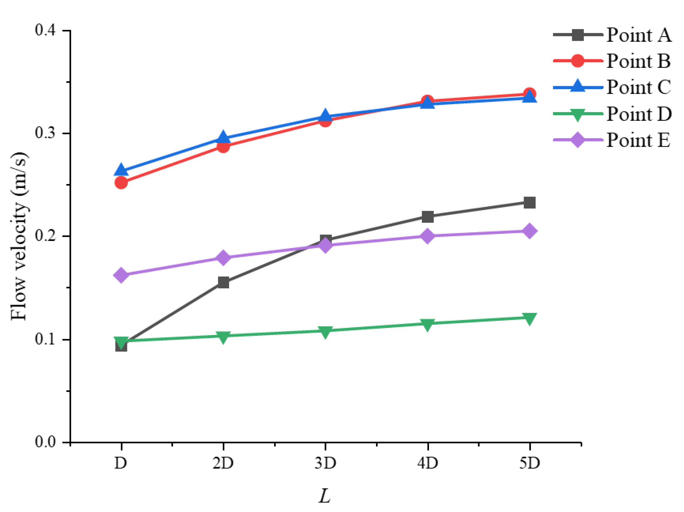
3.3. The effect of Horizontal Distance L on Siltation Characteristics
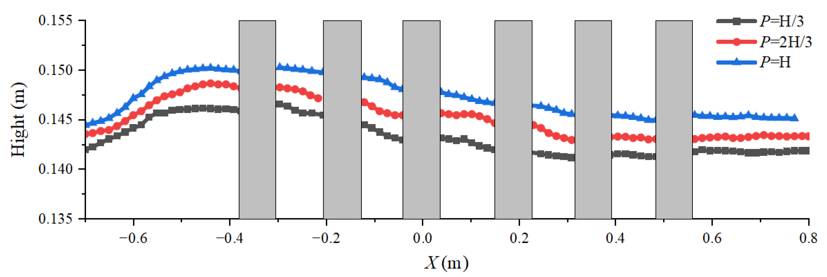
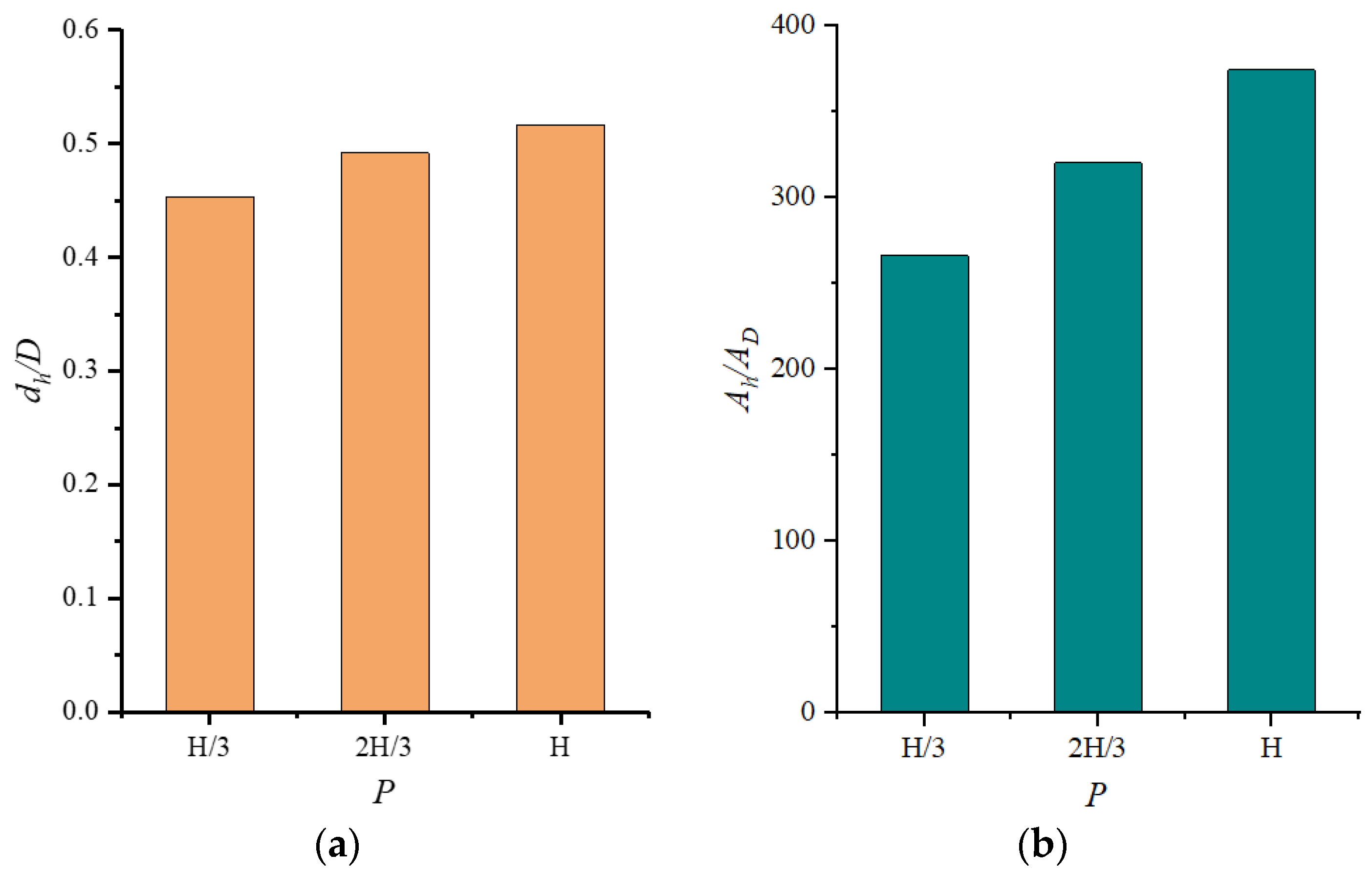
3.4. The Effect of the Height P of the Quasi-Stumps Group on Siltation Characteristics
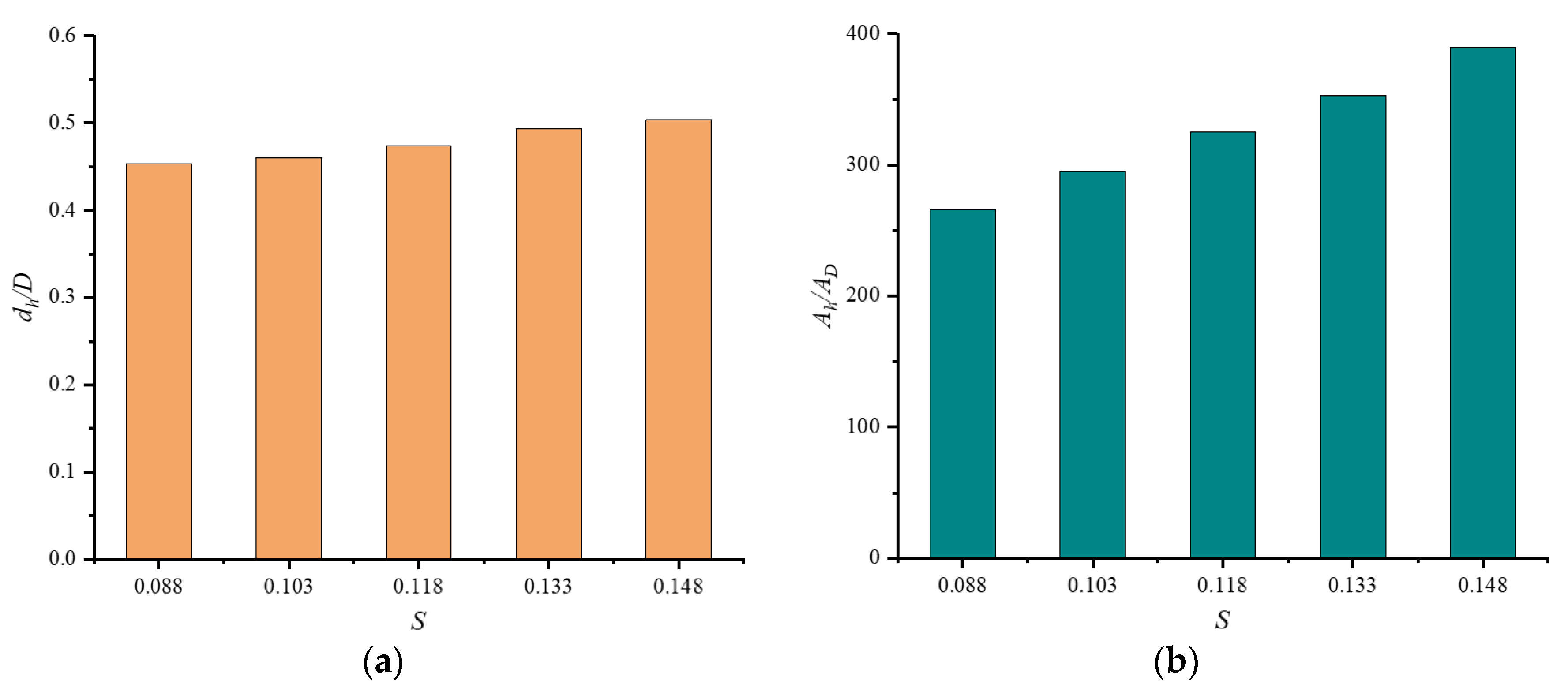
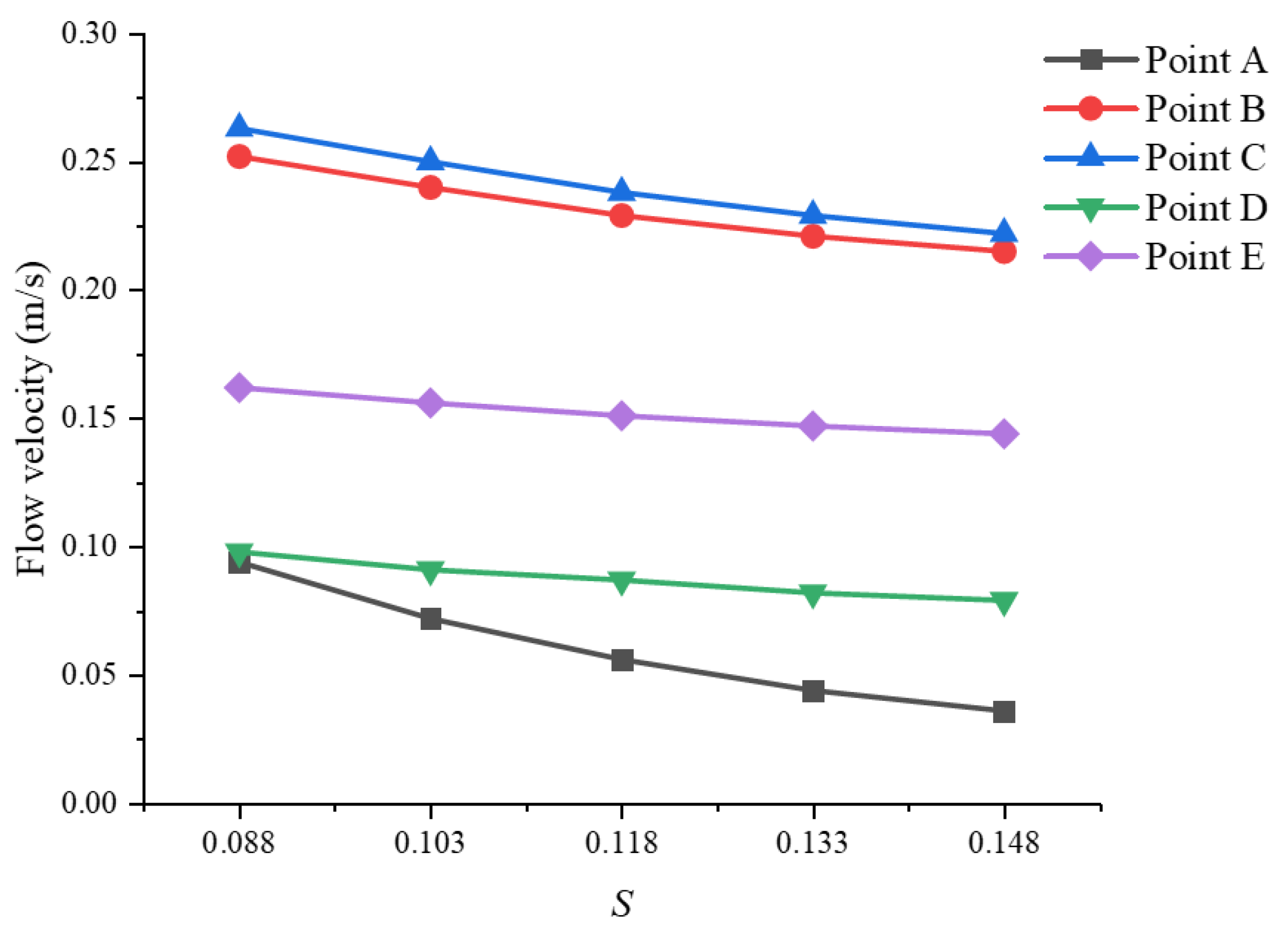
3.5. The Effect of the Ratio S between the Single Leaf Area and the Cross-Sectional Area of Single Pier on the Siltation Characteristics
4. Discussion
5. Conclusions
- (1)
- The results of the numerical simulations using FLOW 3D are in good agreement with the experimental results.
- (2)
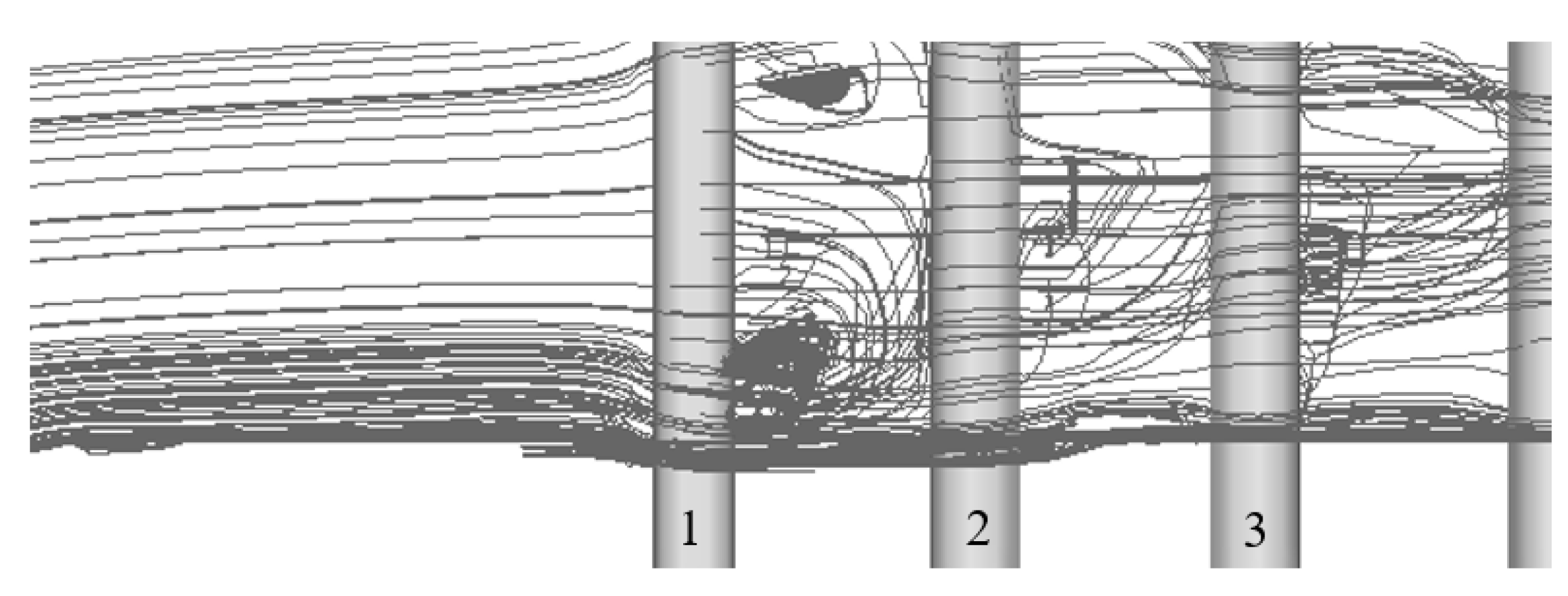
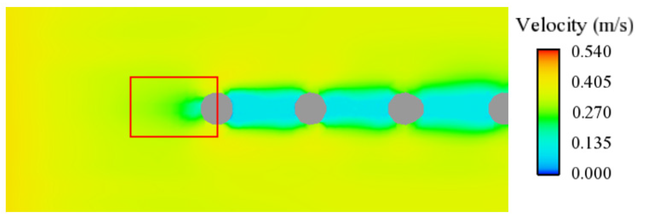
- The presence of the quasi-stumps group can effectively lower the flow velocities around the piers, promote the deposition of suspended sediment, and reduce the sediment scoured from the riverbed. It does not only help safeguard the riverbed around the piers against scouring but also forms siltation, which is beneficial to the stability of the bridge piers.
- (3)
- As the distance L increases, the siltation height at the centerline of the piers group decreases gradually. However, the siltation area and the quantity of the suspended sediment deposition on the entire riverbed gradually increase.
- (4)
- With the increase in the height P and ratio S, the siltation height at the centerline of the piers group, the maximum siltation height, the siltation area, and the quantity of the suspended sediment deposition gradually increase, while the flow velocities around the piers gradually decrease.
- (5)
- The quantity of sediment scoured from the riverbed is less influenced by the L, P, and S.
- (6)
- In this study, the combination of the quasi-stumps group with the best protective effect is P = H, S = 0.148, and L = D.
Author Contributions
Funding
Data Availability Statement
Conflicts of Interest
Appendix A
| Symbol | Meaning |
| Pier diameter | |
| Average velocity upstream of the pier | |
| Water depth | |
| Maximum scouring depth | |
| Average scouring depth | |
| Maximum deposition height | |
| Deposition area | |
| Cross-sectional area of a single pier | |
| Ratio of the area of a single leaf to the cross-sectional area of a single pier | |
| Height of the stumps group in the water | |
| Horizontal distance between the downstream edge of the stumps group and the upstream edge of Pier NO. 1 | |
| RANS | Abbreviation of the Reynolds-averaged Navier–Stokes equation model |
| RNG | Abbreviation of renormalization group |
| k | Turbulent kinetic energy of the turbulence model |
| ε | Turbulent dissipation rate of the k-ε turbulence model |
| ω | Turbulent dissipation rate of the k-ω turbulence model |
| X, Y, Z | Coordinate values in the x, y, and z directions of the coordinate axes are shown in Figure 5a |
References
- Smith, D.W. Why do bridges fail? Civ. Eng. 1977, 47, 58–62. [Google Scholar]
- Lagasse, P.F.; Clopper, P.E.; Zevenbergen, L.W.; Girard, L.G. NCHRP Report 593: Countermeasures to Protect Bridge Piers from Scour; Transportation Research Board: Washington, DC, USA, 2007. [Google Scholar]
- Arneson, L.A.; Zevenbergen, L.W.; Lagasse, P.F.; Clopper, P.E. Evaluating Scour at Bridges, 5th ed.; Bridge Superstructures; U.S. Department of Transportation: Washington, DC, USA, 2012. [Google Scholar]
- Chiew, Y.M. Scour protection at bridge piers. J. Hydraul. Eng. ASCE 1992, 118, 1260–1269. [Google Scholar] [CrossRef]
- Wang, C.; Yu, X.; Liang, F.Y. A review of bridge scour: Mechanism, estimation, monitoring and countermeasures. Nat. Hazards 2017, 87, 1881–1906. [Google Scholar] [CrossRef]
- Jalal, H.K.; Hassan, W.H. Effect of Bridge Pier Shape on Depth of Scour. IOP Conf. Ser. Mater. Sci. Eng. 2020, 671, 12001. [Google Scholar] [CrossRef]
- Jahangirzadeh, A.; Basser, H.; Akib, S.; Karami, H.; Naji, S.; Shamshirband, S. Experimental and Numerical Investigation of the Effect of Different Shapes of Collars on the Reduction of Scour around a Single Bridge Pier. PLoS ONE 2014, 9, e98592. [Google Scholar] [CrossRef] [PubMed]
- Nazari-Sharabian, M.; Nazari-Sharabian, A.; Karakouzian, M.; Karami, M. Sacrificial Piles as Scour Countermeasures in River Bridges a Numerical Study using FLOW-3D. Civ. Eng. J. 2020, 6, 1091–1103. [Google Scholar] [CrossRef]
- Dey, S.; Sumer, B.M.; Fredsoe, J. Control of scour at vertical circular piles under waves and current. J. Hydraul. Eng. 2006, 132, 270–279. [Google Scholar] [CrossRef]
- Kumar, V.; Raju, K.G.R.; Vittal, N. Reduction of local scour around bridge piers using slots and collars. J. Hydraul. Eng. ASCE 1999, 125, 1302–1305. [Google Scholar] [CrossRef]
- Mou, X.; Wang, D.; Ji, H.; Li, C.; Qiao, C. Resistance capability and hydraulic characteristics of ring-wing plates against local scour of round-ended piers. South North Water Transf. Water Sci. Technol. 2017, 15, 146–155. [Google Scholar] [CrossRef]
- Zhang, Y.S.; Wang, J.F.; Zhou, Q.; Li, H.S.; Tang, W. Investigation of the reduction of sediment deposition and river flow resistance around dimpled surface piers. Environ. Sci. Pollut. Res. 2023, 20, 52784–52803. [Google Scholar] [CrossRef]
- Chiew, Y.M. Mechanics of riprap failure at bridge piers. J. Hydraul. Eng. ASCE 1995, 121, 635–643. [Google Scholar] [CrossRef]
- Parola, A.C.; Mahavadi, S.K.; Brown, B.M.; ElKhoury, A. Effects of rectangular foundation geometry on local pier scour. J. Hydraul. Eng. ASCE 1996, 122, 35–40. [Google Scholar] [CrossRef]
- Li, Z.; Tang, H.; Dai, W. Case study of protective effects of ripraps or tetrahedron frame group with different densities on local scour around a pier. J. Sediment Res. 2011, 6, 75–80. [Google Scholar] [CrossRef]
- Jones, J.S.; Kilgore, R.T.; Mistichelli, M.P. Effects of footing location on bridge pier scour. J. Hydraul. Eng. ASCE 1992, 118, 280–290. [Google Scholar] [CrossRef]
- Shilong, F.; Hongwu, T.; Yilin, Z.; Kaixi, C.A.I. Experimental study on effect of local scour at piers and protection by tetrahedron frame. Adv. Water Sci. 2006, 17, 354–358. [Google Scholar] [CrossRef]
- Tabarestani, M.K.; Zarrati, A.R. Design of Stable Riprap around Aligned and Skewed Rectangular Bridge Piers. J. Hydraul. Eng. 2013, 139, 911–916. [Google Scholar] [CrossRef]
- Melville, B.W. Live-bed scour at bridge piers. J. Hydraul. Eng. ASCE 1984, 110, 1234–1247. [Google Scholar] [CrossRef]
- Abt, S.R.; Clary, W.P.; Thornton, C.I. Sediment deposition and entrapment in vegetated streambeds. J. Irrig. Drain. Eng. ASCE 1994, 120, 1098–1111. [Google Scholar] [CrossRef]
- Sun, Z.L.; Zheng, J.Y.; Zhu, L.L.; Chong, L.; Liu, J.; Luo, J.Y. Influence of submerged vegetation on flow structure and sediment deposition. J. Zhejiang Univ. Eng. Sci. 2021, 55, 71–80. [Google Scholar] [CrossRef]
- Nabaei, S.F.; Afzalimehr, H.; Sui, J.Y.; Kumar, B.; Nabaei, S.H. Investigation of the Effect of Vegetation on Flow Structures and Turbulence Anisotropy around Semi-Elliptical Abutment. Water 2021, 13, 3108. [Google Scholar] [CrossRef]
- Amir, M.; Hashmi, H.N.; Baloch, M.; Ehsan, M.A.; Muhammad, U.; Ali, Z. Experimental investigation of channel bank vegetation on scouring characteristics around a wing wall abutment. Mehran Univ. Res. J. Eng. Technol. 2018, 23, 16–22. [Google Scholar]
- Wang, H.; Tang, H.; Zhao, H.; Zhao, X.; Lu, S. Incipient motion of sediment in presence of submerged flexible vegetation. Water Sci. Eng. 2015, 8, 63–67. [Google Scholar] [CrossRef] [Green Version]
- Hongwu, T.; Shengqi, L.U.; Jianchuan, L. Settling velocity of coarse sediment particles in still water with rigid vegetation. J. Hydraul. Eng. 2007, 38, 1214–1220. [Google Scholar] [CrossRef]
- Zhao, H.Q.; Yan, J.; Yuan, S.Y.; Liu, J.F.; Zheng, J.Y. Effects of Submerged Vegetation Density on Turbulent Flow Characteristics in an Open Channel. Water 2019, 11, 2154. [Google Scholar] [CrossRef] [Green Version]
- Xiong, W.; Tang, P.B.; Kong, B.; Cai, C.S. Computational Simulation of Live-Bed Bridge Scour Considering Suspended Sediment Loads. J. Comput. Civ. Eng. 2017, 31, 12. [Google Scholar] [CrossRef]
- Yu, S.L.; Dai, H.C.; Zhai, Y.W.; Liu, M.Y.; Huai, W.X. A Comparative Study on 2D CFD Simulation of Flow Structure in an Open Channel with an Emerged Vegetation Patch Based on Different RANS Turbulence Models. Water 2022, 14, 2873. [Google Scholar] [CrossRef]
- Chen, M.; Lou, S.; Liu, S.; Radnaeva Larisa, D.; Nikitina, E.; Chalov Sergey, R. Numerical Simulation of Wave Propagation and Sediment Suspension Affected by Submerged Rigid Vegetation. J. Tongji Univ. Nat. Sci. 2022, 50, 861–870. [Google Scholar] [CrossRef]
- Asadollahi, M.; Vaghefi, M.; Akbari, M. Effect of the position of perpendicular pier groups in a sharp bend on flow and scour patterns: Numerical simulation. J. Braz. Soc. Mech. Sci. Eng. 2020, 42, 422. [Google Scholar] [CrossRef]
- Bozkus, Z.; Ozalp, M.C.; Dincer, A.E. Effect of Pier Inclination Angle on Local Scour Depth Around Bridge Pier Groups. Arab. J. Sci. Eng. 2018, 43, 5413–5421. [Google Scholar] [CrossRef]
- Heidarpour, M.; Afzalimehr, H.; Izadinia, E. Reduction of local scour around bridge pier groups using collars. Int. J. Sediment Res. 2010, 25, 411–422. [Google Scholar] [CrossRef]
- Saghravani, S.F.; Azhari, A. Simulation of clear water local scour around a group of bridge piers using an Eulerian 3D, two-phase model. Prog. Comput. Fluid Dyn. 2012, 12, 333–341. [Google Scholar] [CrossRef]
- Voskoboinick, A.; Voskoboinick, V.; Turick, V.; Voskoboinyk, O.; Cherny, D.; Tereshchenko, L. Interaction of Group of Bridge Piers on Scour. In Advances in Computer Science for Engineering and Education III. Advances in Intelligent Systems and Computing (AISC 1247); Springer: Berlin/Heidelberg, Germany, 2021; pp. 3–17. [Google Scholar] [CrossRef]
- Jahangirzadeh, A.; Akib, S. Experimental study for determination of collar dimensions around bridge pier. Balt. J. Road Bridge Eng. 2015, 10, 89–96. [Google Scholar] [CrossRef] [Green Version]
- Obied, N.A.; Khassaf, S.I. Experimental Study for Protection of Piers Against Local Scour Using Slots. Int. J. Eng. 2019, 32, 217–222. [Google Scholar] [CrossRef]
- Debnath, K.; Chaudhuri, S. Effect of suspended sediment concentration on local scour around cylinder for clay-sand mixed sediment beds. Eng. Geol. 2011, 117, 236–245. [Google Scholar] [CrossRef]
- Chiew, Y.M.; Melville, B.W. Local scour around bridge piers. J. Hydraul. Res. 1987, 25, 15–26. [Google Scholar] [CrossRef]
- Mastbergen, D.R.; van den Berg, J.H. Breaching in fine sands and the generation of sustained turbidity currents in submarine canyons. Sedimentology 2003, 50, 625–637. [Google Scholar] [CrossRef]
- Soulsby, R. Chapter 9: Bedload transport. In Dynamics of Marine Sands; Ice Publishing: Leeds, UK, 1997; pp. 155–170. [Google Scholar]
- Meyer-Peter, E.; Müller, R. Formulas for bed-load transport. In Proceedings of the 2nd Meeting of the International Association for Hydraulic Structures Research, Delft, The Netherlands, 7 June 1948; pp. 39–64. [Google Scholar]
- Daneshfaraz, R.; Ghaderi, A.; Sattariyan, M.; Alinejad, B.; Asl, M.M.; Di Francesco, S. Investigation of Local Scouring around Hydrodynamic and Circular Pile Groups under the Influence of River Material Harvesting Pits. Water 2021, 13, 2192. [Google Scholar] [CrossRef]
- Kim, H.S.; Roh, M.; Nabi, M. Computational Modeling of Flow and Scour around Two Cylinders in Staggered Array. Water 2017, 9, 654. [Google Scholar] [CrossRef] [Green Version]
- Wang, F.; Zhang, B.; Qi, J. 3D numerical investigation of bridge pier-scour development using a dynamic-mesh updating technique. South North Water Transf. Water Sci. Technol. 2017, 15, 132–137. [Google Scholar] [CrossRef]
- Wang, S.H.; Yang, S.Y.; He, Z.G.; Li, L.; Xia, Y.Z. Effect of Inclination Angles on the Local Scour around a Submerged Cylinder. Water 2020, 12, 2687. [Google Scholar] [CrossRef]
- Li, J.Z.; Kong, X.; Yang, Y.L.; Deng, L.; Xiong, W. CFD investigations of tsunami-induced scour around bridge piers. Ocean Eng. 2022, 244, 16. [Google Scholar] [CrossRef]
- Li, A.; Zhang, G.; Chandara, M.; Zhou, S. Influence of sediment transport rate formula on numerical simulation of local scour around a bridge pier. J. Sediment Res. 2022, 47, 15–22. [Google Scholar] [CrossRef]
- Sheppard, D.M.; Odeh, M.; Glasser, T. Large scale clear-water local pier scour experiments. J. Hydraul. Eng. 2004, 130, 957–963. [Google Scholar] [CrossRef]


| Test Number | Mesh Size (m) | Mesh Number | Numerical Simulation | Laboratory Experiment | Mean Error | ||
|---|---|---|---|---|---|---|---|
| 1 | 0.016 | 216,384 | 0.0178 | 0.0153 | 0.0159 | 0.0134 | 13.1% |
| 2 | 0.014 | 305,133 | 0.0171 | 0.0145 | 7.9% | ||
| 3 | 0.012 | 491,175 | 0.0166 | 0.0141 | 4.8% | ||
| 4 | 0.010 | 855,360 | 0.0166 | 0.0140 | 4.5% | ||
| Experimental Number | (m/s) | (m) | |||
|---|---|---|---|---|---|
| 0 | 0.48 | 0.24 | Without quasi-stumps group | ||
| 1 | 0.088 | H/3 | D | ||
| 2 | 0.088 | H/3 | 2D | ||
| 3 | 0.088 | H/3 | 3D | ||
| 4 | 0.088 | H/3 | 4D | ||
| 5 | 0.088 | H/3 | 5D | ||
| 6 | 0.088 | 2H/3 | D | ||
| 7 | 0.088 | H | D | ||
| 8 | 0.103 | H/3 | D | ||
| 9 | 0.118 | H/3 | D | ||
| 10 | 0.133 | H/3 | D | ||
| 11 | 0.148 | H/3 | D | ||
| Relative Error | Experiment NO. 0 | Relative Error | Experiment NO. 5 | Relative Error | Experiment NO. 10 | Relative Error | ||||
|---|---|---|---|---|---|---|---|---|---|---|
| Points | Experiment | Numerical Simulation | Experiment | Numerical Simulation | Experiment | Numerical Simulation | ||||
| Point A | 0.341 | 0.332 | −2.64% | 0.233 | 0.253 | 8.58% | 0.044 | 0.045 | 2.27% | |
| Point B | 0.447 | 0.423 | −5.37% | 0.338 | 0.354 | 4.73% | 0.221 | 0.219 | −0.90% | |
| Point C | 0.438 | 0.411 | −6.16% | 0.334 | 0.347 | 3.89% | 0.229 | 0.225 | −1.75% | |
| Point D | 0.147 | 0.144 | −2.04% | 0.121 | 0.123 | 1.65% | 0.082 | 0.085 | 3.66% | |
| Point E | 0.253 | 0.254 | 0.40% | 0.205 | 0.206 | 0.49% | 0.147 | 0.148 | 0.68% | |
Disclaimer/Publisher’s Note: The statements, opinions and data contained in all publications are solely those of the individual author(s) and contributor(s) and not of MDPI and/or the editor(s). MDPI and/or the editor(s) disclaim responsibility for any injury to people or property resulting from any ideas, methods, instructions or products referred to in the content. |
© 2023 by the authors. Licensee MDPI, Basel, Switzerland. This article is an open access article distributed under the terms and conditions of the Creative Commons Attribution (CC BY) license (https://creativecommons.org/licenses/by/4.0/).
Share and Cite
Zhang, Y.; Wang, J.; Zhou, Q.; Cai, Y.; Tang, W. The Investigation of Local Scour around Bridge Piers with the Protection of a Quasi-Stumps Group. Water 2023, 15, 2858. https://doi.org/10.3390/w15152858
Zhang Y, Wang J, Zhou Q, Cai Y, Tang W. The Investigation of Local Scour around Bridge Piers with the Protection of a Quasi-Stumps Group. Water. 2023; 15(15):2858. https://doi.org/10.3390/w15152858
Chicago/Turabian StyleZhang, Yisheng, Jiangfei Wang, Qi Zhou, Yingchun Cai, and Wei Tang. 2023. "The Investigation of Local Scour around Bridge Piers with the Protection of a Quasi-Stumps Group" Water 15, no. 15: 2858. https://doi.org/10.3390/w15152858
APA StyleZhang, Y., Wang, J., Zhou, Q., Cai, Y., & Tang, W. (2023). The Investigation of Local Scour around Bridge Piers with the Protection of a Quasi-Stumps Group. Water, 15(15), 2858. https://doi.org/10.3390/w15152858