Applying Adaptive Neuro-Fuzzy Inference System to Improve Typhoon Intensity Forecast in the Northwest Pacific

Abstract

Typhoon intensity forecast is an important issue. The objective of this study is to construct a 5-day 12-hourly typhoon intensity forecast model based on the adaptive neuro-fuzzy inference systems (ANFIS) to improve the typhoon intensity forecast in the Northwest Pacific. It analyzed the improvement of the ANFIS typhoon intensity forecast model by comparing it with the MLR model when only the atmospheric factor or both atmospheric and oceanic factors are considered. This study collected the SHIPS (Statistical Hurricane Intensity Prediction Scheme) developmental data of typhoons in the Northwest Pacific before landing from 2000 to 2012. The input factors of the ANFIS model were simplified by the stepwise regression procedure (SRP). Subtractive clustering (SC) was used to determine the number of ANFIS rules and to reduce model complexity. Model Index (MI) was taken as the clustering standard of SC to determine the network architecture of the ANFIS typhoon intensity forecast model. The simulated results show that the MI could effectively determine the radius of influence of SC. The typhoon intensity forecast was significantly improved after oceanic environmental factors were added. The improvement of RMSE of ANFIS was the highest at 84 h; the improvement of ANFIS on the underestimated ratio was primarily positive. The Typhoon Songda case study shows that the maximum bias of ANFIS is greatly improved, at 60 h of the lead time, and the improvement percentage of maximum bias is the highest (39%). Overall, the ANFIS model could effectively improve the MLR model in typhoon intensity forecast.

1. Introduction

Taiwan, located in the Northwest Pacific and at the boundary of temperate and subtropical zones, is often hit by typhoons. The terrain of Taiwan is mostly hillsides with short and fast-flowing rivers. Typhoons cause economic losses in agriculture, fishery, and animal husbandry and cause casualties yearly. This type of loss is mostly caused by the heavy rainfall that occurs with a typhoon. If a high-intensity typhoon hits, the disaster will be more serious. The quality of typhoon forecasting plays an important role in preventing and reducing major disasters.

Typhoon intensity prediction is one of the important items of typhoon forecast as stronger typhoons can cause more severe disasters. However, an accurate forecast is difficult due to complex thermal and dynamical conditions (namely, environmental factors, such as atmosphere and ocean) for typhoon development [1,2]. The US Navy’s Joint Typhoon Warning Center (JTWC) uses an ST5D statistical model as the baseline to evaluate the intensity forecast technology. The ST5D model applies the concepts of climate and CLIPER to estimate the 5-day typhoon intensity without considering the possible track in the future. It will significantly underestimate the effects of typhoon intensity over time. DeMaria et al. [2] pointed out that though the typhoon intensity forecast technology is steadily improved, it still lags the typhoon track forecast technology.

Statistical and dynamical models are commonly used for typhoon intensity forecasts worldwide. Common statistical models based on CLIPER include SHIFOR (Statistical Hurricane Intensity Forecast Model) [3] and SHF5 (namely, 5-day 6-hourly SHIFOR) [4,5,6,7,8,9]. Dynamical models include GFDI, GHMI, and HWFI (coupled atmosphere-ocean model) [2]. Due to complex changes in typhoon intensity, statistical models based on CLIPER often struggle to accurately describe the interaction between atmospheric and oceanic environmental factors and typhoon intensity. In contrast, numerical weather models (namely, dynamical models) can describe the interaction between atmospheric and oceanic environmental factors and typhoon intensity. However, as typhoons are mesoscale weather systems, there is still room for improvement in dynamical models’ ability to simulate detailed typhoon structures. Besides statistical and dynamical models, there is a statistical dynamical approach that combines statistical methods with environmental factors output by the numerical weather forecast. SHIPS (Statistical Hurricane Intensity Prediction Scheme) [1] is used in the North Atlantic and Eastern Pacific. The results show that the error of SHIPS is smaller than that of models based on climate and persistency. STIPS (Statistical Typhoon Intensity Prediction Scheme), proposed by Knaff et al. [10], is a multiple linear regression (MLR) model developed for the Northwest Pacific and takes the synoptic-scale environmental variable of global models as forecast factors [10].

The statistical dynamical approach (such as SHIPS and STIPS) mainly uses atmospheric and oceanic environmental factors output by dynamical models as predictors of MLR to forecast changes in typhoon intensity. The interaction of atmospheric and oceanic environmental factors with changes in typhoon intensity is a highly nonlinear system. MLR cannot effectively analyze the nonlinear relationship [11]. Machine learning (ML) can learn and simulate nonlinear systems more effectively than MLR [12]. Common ML methods are an artificial neural network (ANN) [13,14,15,16] and a fuzzy inference system (FIS). A study has shown that ANN is superior to MLR in estimating the depth of the oceanic mixing layer [17]. By combining genetic algorithms and artificial neural networks, Jin et al. obtained a more efficient method in intensity forecasting than climate and persistency [18]. Sharma et al. employed ANN to develop a soft-computing cyclone intensity prediction scheme (SCIPS) which, as with STIPS, is a model to forecast typhoon intensity in the Northwest Pacific [11]. They used ANN to improve the typhoon intensity forecasting in the Northwest Pacific and attempted to take the ocean heat content (OHC) as a predictor. SCIPS improves the previously widely used MLR intensity forecast model. Its performance is improved with increasing intensity and lead time when compared with MLR.

FIS is widely applied in studies on a hydrometeorological forecast to simulate the nonlinear relationship [13,19,20]. Jang developed adaptive neuro-fuzzy inference systems (ANFIS) with the combination of artificial neural networks, which optimizes parameters through self-learning and organizational abilities of artificial neural networks [21]. In recent years, ANFIS has been widely used in hydrometeorology. The research results show that ANFIS can provide reliable and stable hydrological forecasts [22,23,24,25].

As mentioned above, the main objective of this paper is that a typhoon intensity forecasting model proposed to utilize the typhoon dataset, SHIPS, from the statistical and dynamical models to improve the method by Knaff et al. However, this study does not specifically analyze the prediction of rapid intensification (RI) of typhoons. The ANFIS is employed to construct a typhoon intensity forecast model, including both the thermal and dynamical conditions, for predicting every 12 h for the next five days to improve the accuracy and quality of typhoon intensity forecast. The stepwise regression procedure (SRP) was employed to simplify model input data and reduce model complexity. A benchmark model was built based on the Knaff’s MLR approach in order to analyze and compare the performance of the ANFIS typhoon intensity forecast, which gives predictions every 12 h for the coming five days.

2. Methodology

2.1. Subtractive Clustering

An important step in ANFIS is to determine the number of fuzzy rules. If rules increase, parameters will increase, and models will become more complex and take longer to build. Clustering can effectively distinguish the correlation with each cluster with a small number of rules, such as fuzzy C-means and subtractive clustering (SC) [26]. Studies on ANFIS demonstrate that good performances can be achieved if SC is used to determine the number of rules [27,28]. Therefore, SC was used in this study to determine the fuzzy rules of ANFIS.

In SC, each data point is considered a potential clustering center. The center of the place with the densest data is selected as the most representative clustering center. This center point and its surrounding data points are eliminated to correct the density of the data point. Afterwards, the next clustering center is selected and eliminated until all conditions are met. The calculated amount of subtraction clustering does not change with the complexity of systems but is proportional to the number of data groups [29].

Assuming that there are n groups of data X_i (i = 1, 2, …, n) in M-dimensional space, the density measure D_i is defined as shown in Equation (1):

$$D_i=\sum _{j=1}^{n}exp\left(-\frac{{‖X_i-X_j‖}^2}{{(r_a/2)}^2}\right)$$

(1)

where r_a is the radius of influence. The density measure of each point (X_i) is calculated, and the point with the highest density measure is selected as the first clustering center point (X_c1). The correction is continued until X_ck is Clustering Center k. The equation of D_ck is shown in Equation (2):

$$D_i=D_i-D_{ck}exp\left(-\frac{{‖X_i-X_{ck}‖}^2}{{(r_b/2)}^2}\right)$$

(2)

where r_b is the correction radius, which is set to avoid the next clustering center being too close to the previous center point. Generally, the recommended value of r_b is 1.5r_a. After selecting the second clustering center point, the calculation equation is corrected to calculate the next clustering center point until the stop condition is met.

2.2. Adaptive Neuro-Fuzzy Inference Systems

ANFIS combines FIS with neural network architecture to ensure FIS has self-organizing and learning abilities to adjust model parameters [29]. The if-then rule is mainly set in first-order Sugeno fuzzy models (functional fuzzy). Its architecture is shown in Figure 1 and explained as follows.

1.

Input layer:

Artificial neurons map input variables to fuzzy sets by calculating compatibility between input data and fuzzy sets, as shown in Equation (3):

$$O_{1,ji}={\mu }_j\left(x_i\right)=\exp \left(-\frac{{‖x_i-c_{ji}‖}^2}{2{\sigma }_{ji}^2}\right) for i=\mathrm{1,2},\dots ,N;j=\mathrm{1,2},\dots ,M_i$$

(3)

where $O_{1,ji}$ is the output from the input layer to the rules layer and ${\mu }_j\left(x_i\right)$ is the membership function of Set j of Input Variable i. A Gaussian membership function was used in this study, in which $c_{ji} \mathrm{and} {\sigma }_{ji}$ are premise parameters.

2.

Rules layer:

Artificial neurons, labeled Π, calculate the fuzzy rule AND, as shown in Equation (4):

$$O_{2,p}=w_p=\prod _{i=1}^N{\mu }_{pi}\left(x_i\right) for \mathrm{p}=1,\dots ,\mathrm{P}$$

(4)

where $O_{2,p}$ is the output from the rules layer to the normalization layer. $w_p$ is the weight, and P is the total number of rules. SC was adopted in this study to determine P.

3.

Normalization layer:

Artificial neurons, labeled N, calculate the normalization, as shown in Equation (5):

$$O_{3,p}={\overline{w}}_p=\frac{w_p}{\sum _{p=1}^p{w}_p}$$

(5)

where $O_{3,p}$ is the output from the normalization layer to the inference layer.

4.

Defuzzification layer:

The normalized results obtained from the previous layer are multiplied by Sugeno fuzzy model, as shown in Equation (6):

$$O_{4,p}={\overline{w}}_p{f}_p={\overline{w}}_p\left(\sum _{i=0}^N{r}_{pi}{x}_i\right)$$

(6)

where $O_{4,p}$ is the output from the inference layer to the output layer and $r_{pi}$ is the conclusion parameter.

5.

Output layer:

There is only a single neuron, labeled Σ. The total output of neurons in the previous layer was calculated as the final output of the network, as shown in Equation (7):

$$O_{\mathrm{5,1}}=\sum _{p=1}^P{\overline{w}}_p{f}_p=\frac{\sum _{p=1}^P{w}_p{f}_p}{\sum _{p=1}^P{w}_p}$$

(7)

where $O_{\mathrm{5,1}}$ is the final output.

Setting fuzzy rules and membership is an important step in ANFIS. This study used SC to determine fuzzy rules and their membership. SC is based on its clustering center, and its results mainly affect radius (r_a).

3. Data and Assessment Indicators

3.1. Typhoon Best Track Data

The US JTWC issues warnings for tropical cyclones in the Pacific Ocean, Indian Ocean, and other sea areas. In this study, tropical cyclone best track data on the JTWC website were selected, including the latitude and longitude of typhoon centers and the maximum wind speed of typhoons.

3.2. SHIPS Development Data

SHIPS uses environmental predictors, such as vertical wind shear and ocean heat content, to forecast changes in typhoon intensity (DELV) with MLR. SHIPS has been proven effective for the forecast in the North Atlantic and Eastern Pacific [2]. It provides information about predictors affecting the change of typhoon intensity.

The SHIPS developmental data comprises meteorological factors that may be used in STIPS. These data are summarized according to typhoon events, including data from the first 12 h before and the next 120 h after each observation. The data also include the typhoon intensity and center location provided by the NHC (National Hurricane Center), JTWC, National Centers for Environmental Prediction (NCEP) reanalysis data, and environmental factors of the typhoon vicinity for the global forecast system. SHIPS development data also include oceanic environmental factors such as ocean heat content and surface sea temperature. Detailed STIPS developmental data are available on the Regional and Mesoscale Meteorology Branch’s website (https://rammb2.cira.colostate.edu/research/tropical-cyclones/ships/, accessed on 31 July 2023). The primary data of this study were sourced from the typhoon data in the Northwest Pacific, which were added to SHIPS developmental data (2000–2012).

3.3. STIPS

STIPS, developed by [10] for typhoon intensity forecast in the Northwest Pacific, is closely related to SHIPS, proposed by DeMaria and Kaplan [30]. STIPS is an MLR model, and the dependent variable (forecast value) is the change of 12-hourly typhoon intensity at the initial forecast time (DELV) before typhoon landfall. STIPS selects the important factors at each forecast time by a stepwise procedure. The selected factors include DVMAX (12-h intensity change), SPD (typhoon speed), VMAX (initial typhoon intensity), VMAX² (squared initial typhoon intensity), MPI (maximum potential typhoon intensity), MPI² (squared maximum potential typhoon intensity), MPI × VMAX, SHRD (vertical wind shear at 200–850 hPa), USHRD (vertical shear of zonal wind at 200–850 hPa), T200 (the temperature at 200 hPa), and RHHI (average relative humidity at 500–300 hPa). In this study, STIPS was taken as the benchmark model, and the factors used in STIPS were adopted. USHRD could not be obtained in STIPS developmental data and thus was not included in this study.

3.4. Research Data Grouping

This study selected typhoon data in the Northwest Pacific before landfall from 2000 to 2012 as case study. The data were divided into ten groups with 12 to 120 h of lead time at 12-h intervals. Typhoon data were sourced from observed values of JTWC and STIPS developmental data in the Northwest Pacific. Typhoon data were selected from 335 events, and their tracks are shown in Figure 2. In ANFIS, data from 2000 to 2005 was the training data, from 2006 to 2008 was the validation data, and from 2009 to 2012 was the testing data.

Input variables/factors of the ANFIS model in this study were based on the factors of STIPS, and the factor of the statistical forecasts model that Lin [31] proposed has been considered in this study. Atmospheric and oceanic factors of SHIPS developmental data were also included. The data were grouped into SHIPSa and SHIPSb. SHIPSa only contained atmospheric factors, and SHIPSb was based on SHIPSa with oceanic factors added. Detailed predictors are shown in

Table 1. Input factor candidate list.

Factor	Description	SHIPSa	SHIPSb
VMAX	Maximum surface wind (kt)	O	O
VMAX2	Maximum surface wind square (kt)	O	O
DVMAX	12 h change in intensity	O	O
LON	Storm longitude (deg $W\times 10$) vs. time	O	O
LAT	Storm latitude (deg $W\times 10$) vs. time	O	O
SPD	Storm center moving speed	O	O
MPI	Maximum potential intensity from Kerry Emanuel equation (kt)	O	O
MPI2	Maximum potential intensity square from Kerry Emanuel equation (kt)	O	O
MPI $\times$ VMAX	MPI times the initial intensity	O	O
POT	MPI and VMAX difference	O	O
SHRD	850–200 hPa shear magnitude (kt $\times$ 10) vs. time (r = 200–800 km)	O	O
SHRS	850–500 hPa shear magnitude (kt $\times$ 10) vs. time	O	O
T200	Same as above for 200 hPa temperature (deg C $\times$ 10)	O	O
U200	200 hPa zonal wind (kt $\times$ 10) vs. time (r = 200–800 km)	O	O
RHLO	850–700 hPa relative humidity (%) vs. time (r = 200–800 km)	O	O
RHHI	Same as RHLO for 500–300 hPa	O	O
RSST	Reynolds SST (deg C $\times$ 10) vs. time. Number after SST label is the age in days of the SST analysis used to estimate RSST.		O
SSTA	Sea surface temperature anomaly of storm center		O
RSSTd12	12 h change in RSST		O
RSSTd24	24 h change in RSST		O
SSTAd24	12 h change in SSTA		O
RHCN	Ocean heat content ($KJ/{\mathrm{c}\mathrm{m}}^2$) from satellite altimetry data		O
RHCNd12	12 h change in RHCN		O
RHCNd24	24 h change in RHCN		O
OHCA	Ocean heat content anomaly of storm center		O
OHCAd24	24 h change in OHCA		O
ATCHP	Accumulated tropical cyclone heat potential		O
TOHC	24 h RHCN cumulative value		O
TOHA	24 h RHCN cumulative value and climatic cumulative value difference		O

. The model’s output value is the change of typhoon intensity at the initial forecast time (DELV).

3.5. Model Performance Indicators

The model performance indicators used in this study are as follows.

1.

Root Mean Square Error (RMSE)

$$\mathrm{R}\mathrm{M}\mathrm{S}\mathrm{E}={\left[\frac{{\sum }_{\mathrm{i}=1}^{\mathrm{n}}{({\mathrm{Y}}_{\mathrm{i}}-{\mathrm{F}\mathrm{Y}}_{\mathrm{i}})}^2}{\mathrm{n}}\right]}^{\frac{1}{2}}$$

(8)

where n is the number of data groups, Yi is the observed typhoon intensity, and FYi is the forecast typhoon intensity. A small RMSE leads to a small error between the observed and the forecast values.

2.

Improvement Percentage of RMSE (IPRMSE)

$$\mathrm{I}\mathrm{P}\mathrm{R}\mathrm{M}\mathrm{S}\mathrm{E}=\frac{{\mathrm{F}\mathrm{Y}}_{\mathrm{M}\mathrm{L}\mathrm{R}}-{\mathrm{F}\mathrm{Y}}_{\mathrm{A}\mathrm{N}\mathrm{F}\mathrm{I}\mathrm{S}}}{{\mathrm{F}\mathrm{Y}}_{\mathrm{M}\mathrm{L}\mathrm{R}}}\times 100\%$$

(9)

where ${\mathrm{F}\mathrm{Y}}_{\mathrm{A}\mathrm{N}\mathrm{F}\mathrm{I}\mathrm{S}}$ is the typhoon intensity forecasted by ANFIS and ${\mathrm{F}\mathrm{Y}}_{\mathrm{M}\mathrm{L}\mathrm{R}}$ is the typhoon intensity forecasted by the MLR model.

3.

Underestimated Ratio (UR)

The underestimated ratio is the percentage of the observed value of the evaluation model to the forecast value. The equation is shown as follows:

$$\mathrm{U}\mathrm{R}=\frac{\mathrm{N}\mathrm{u}\mathrm{m}\mathrm{b}\mathrm{e}\mathrm{r}\mathrm{s} \mathrm{o}\mathrm{f} \mathrm{d}\mathrm{a}\mathrm{t}\mathrm{a} \mathrm{s}\mathrm{m}\mathrm{a}\mathrm{l}\mathrm{l}\mathrm{e}\mathrm{r} \mathrm{t}\mathrm{h}\mathrm{a}\mathrm{n} \mathrm{t}\mathrm{h}\mathrm{e} \mathrm{p}\mathrm{r}\mathrm{e}\mathrm{d}\mathrm{i}\mathrm{c}\mathrm{t}\mathrm{a}\mathrm{n}\mathrm{d}}{\mathrm{T}\mathrm{o}\mathrm{t}\mathrm{a}\mathrm{l} \mathrm{n}\mathrm{u}\mathrm{m}\mathrm{b}\mathrm{e}\mathrm{r} \mathrm{o}\mathrm{f} \mathrm{d}\mathrm{a}\mathrm{t}\mathrm{a}}\times 100\%$$

(10)

The forecast value is underestimated if the underestimated ratio is close to 100. Otherwise, if the underestimated ratio is close to 0, the forecast value is less underestimated.

4.

Improvement Percentage of UR (IPUR)

$$\mathrm{I}\mathrm{P}\mathrm{U}\mathrm{R}=\frac{{\mathrm{F}\mathrm{Y}}_{\mathrm{M}\mathrm{L}\mathrm{R}}-{\mathrm{F}\mathrm{Y}}_{\mathrm{A}\mathrm{N}\mathrm{F}\mathrm{I}\mathrm{S}}}{{\mathrm{F}\mathrm{Y}}_{\mathrm{M}\mathrm{L}\mathrm{R}}}\times 100\%$$

(11)

where ${\mathrm{F}\mathrm{Y}}_{\mathrm{A}\mathrm{N}\mathrm{F}\mathrm{I}\mathrm{S}}$ is the typhoon intensity forecasted by ANFIS, and ${\mathrm{F}\mathrm{Y}}_{\mathrm{M}\mathrm{L}\mathrm{R}}$ is the typhoon intensity forecasted by the MLR model.

5.

Maximum Absolute Error (MAE) and best Model Index (MI)

$$\mathrm{M}\mathrm{A}\mathrm{E}=\mathrm{m}\mathrm{a}\mathrm{x}\left(\left|\mathrm{F}\mathrm{Y}-\mathrm{Y}\right|\right)$$

(12)

where Y is the observed typhoon intensity, and FY is the forecasted typhoon intensity.

$$\mathrm{MI}=|\mathrm{T}\mathrm{r}\mathrm{n}\mathrm{M}\mathrm{A}\mathrm{E}-\mathrm{V}\mathrm{a}\mathrm{l}\mathrm{M}\mathrm{A}\mathrm{E}|$$

(13)

To avoid overfitting or underfitting, MI is an indicator to select the optimal ANFIS. $\mathrm{T}\mathrm{r}\mathrm{n}\mathrm{M}\mathrm{A}\mathrm{E}$ is the maximum absolute error of training data, and $\mathrm{V}\mathrm{a}\mathrm{l}\mathrm{M}\mathrm{A}\mathrm{E}$ is the maximum absolute error of validation data. MI can determine the hyperparameter combination of the optimal ANFIS.

6.

Bias (B)

$$\mathrm{B}=\mathrm{F}\mathrm{Y}-\mathrm{Y}$$

(14)

where Y is the observed typhoon intensity, and FY is the forecast typhoon intensity. The bias can show the difference between the forecast and the observed values.

7.

Improvement Percentage of Bias (IPB)

$$\mathrm{I}\mathrm{P}\mathrm{B}=\frac{{\mathrm{F}\mathrm{Y}}_{\mathrm{M}\mathrm{L}\mathrm{R}}-{\mathrm{F}\mathrm{Y}}_{\mathrm{A}\mathrm{N}\mathrm{F}\mathrm{I}\mathrm{S}}}{{\mathrm{F}\mathrm{Y}}_{\mathrm{M}\mathrm{L}\mathrm{R}}}\times 100\%$$

(15)

where ${\mathrm{F}\mathrm{Y}}_{\mathrm{A}\mathrm{N}\mathrm{F}\mathrm{I}\mathrm{S}}$ is the typhoon intensity forecast by ANFIS, and ${\mathrm{F}\mathrm{Y}}_{\mathrm{M}\mathrm{L}\mathrm{R}}$ is the typhoon intensity forecast by the MLR model.

4. Typhoon Intensity Forecast Model Construction

4.1. Selection of Input Factors for Typhoon Intensity Forecast Models

In this study, input factors of ANFIS were selected by SRP. SRP can be divided into forward selection, backward selection, and stepwise selection according to selection methods. Stepwise selection, combining forward and backward selection, first selects predictors by forward selection and then conducts tests by backward selection.

SRP is used to select a variable combination with maximum explanatory power. It selects input variables according to the regression analysis of input and output variables and the performance of the linear regression test on the variable combination. It selects variables that pass the F-test by forward selection and removes variables that fail to pass the F-test by backward selection. After SRP’s F-test of the input variable combination, the t-test of a causal relationship between independent and dependent variables is conducted.

The input variables selected by SRP for the SHIPSa 12-h forecast model are shown in

Table 2. Results of SHIPSa with SRP (lead time = 12 h).

SHIPSa (Lead Time = 12 h)
Variable Selected	t-Test	p-Value	F-Test	p-Value
VMAX	−5.7833	7.89 × 10−9	328.747221	<0.05
${\mathrm{V}\mathrm{M}\mathrm{A}\mathrm{X}}^2$	−16.5477	1.56 × 10−59
DVMAX	25.1782	6.26 × 10−130
LON	5.6361	1.86 × 10−8
${\mathrm{M}\mathrm{P}\mathrm{I}}^2$	3.5526	3.86 × 10−4
MPI × VMAX	10.4321	3.73 × 10−25
POT	−4.0242	5.82 × 10−5
SHRD	−13.4377	2.71 × 10−40
T200	−7.8727	4.44 × 10−15
RHLO	5.2101	1.98 × 10−7

, including VMAX (initial typhoon intensity), VMAX2 (squared initial typhoon intensity), DVMAX (intensity difference 12 h before typhoon), LON (longitude of typhoon center at the current moment), MPI2 (squared maximum potential typhoon intensity), MPI × VMAX (maximum potential typhoon intensity times initial typhoon intensity), POT (difference between maximum potential typhoon intensity times initial intensity), SHRD (vertical wind shear at 850–200 mb), T200 (the average temperature at 200 mb), and RHLO (relative humidity at 850–700 mb). Based on the input variables selected by SRP for SHIPSa 12 to 120-h forecast models,

Table 3. The factor selected by SRP in each lead time for SHIPSa.

	Variable Sequence of SRP
Lead Time (h)	1	2	3	4	5	6	7	8	9	10
12	DVMAX	POT	SHRD	LON	MPI $\times$ VMAX	VMAX2	T200	RHLO	VMAX	MPI2
24	POT	DVMAX	SHRD	LON	VMAX2	MPI $\times$ VMAX	T200	RHLO	MPI	MPI2
36	POT	DVMAX	SHRD	LON	MPI $\times$ VMAX	VMAX2	T200	RHLO	SHRS	LAT
48	POT	DVMAX	SHRD	LON	VMAX2	MPI $\times$ VMAX	T200	RHLO	SHRS	LAT
60	POT	DVMAX	LON	SHRD	VMAX2	MPI $\times$ VMAX	T200	RHLO	RHHI
72	POT	LON	DVMAX	VMAX2	MPI2	SHRD	T200	RHLO	RHHI
84	POT	LON	DVMAX	VMAX2	MPI2	RHHI	T200	SHRD	SHRS
96	POT	LON	VMAX2	RHHI	SHRD	T200	MPI2	MPI × VMAX	SHRS	DVMAX
108	POT	LON	VMAX2	RHHI	T200	SHRD	MPI2	MPI × VMAX	SHRS	SPD
120	POT	LON	VMAX2	RHHI	SHRD	T200	SHRS	SPD	RHLO	DVMAX

shows the order of factors selected for SHIPSa in all forecast periods. The numbers at the top of the table indicate the selection order by SRP, and the numbers at the left of the table indicate the 12 to 120-h forecast models. According to the selection results, POT has an important influence on various forecast models. VMAX2 and LON enhance their influences over the lead time, and DVMAX and SHRD lose their influences with an increase in the lead time.

The input variables selected by SRP for the SHIPSb 12-h forecast model are shown in

Table 4. Results of SHIPSb with SRP (lead time = 12 h).

SHIPSb (Lead time = 12 h)
Variable Selected	t-Test	p-Value	F-Test	p-Value
VMAX	−4.9259	8.74 × 10−7	329.0337491	<0.05
VMAX2	−16.7533	6.27 × 10−61
DVMAX	24.7237	1.15 × 10−125
LON	5.3472	9.43 × 10−8
MPI × VMAX	10.9866	1.10 × 10−27
POT	−3.1612	1.58 × 10−3
SHRD	−13.1414	1.20 × 10−38
T200	−7.3629	2.18 × 10−13
RHLO	5.2744	1.40 × 10−7
RHCN	3.7676	1.67 × 10−4

, including VMAX (initial typhoon intensity), VMAX² (squared initial typhoon intensity), DVMAX (intensity difference 12 h before typhoon), LON (longitude of typhoon center at the current moment), MPI × VMAX (maximum potential typhoon intensity times initial typhoon intensity), POT (difference between maximum potential typhoon intensity times initial intensity), SHRD (vertical wind shear at 850–200 mb), T200 (the average temperature at 200 mb), RHLO (relative humidity at 850–700 mb), and RHCN (ocean heat content). The words in bold are oceanic environmental factors. Based on the input variables selected by SRP for the SHIPSa forecast models for 12 to 120 h,

Table 5. The factor selected by SRP in each lead time for SHIPSb.

	Variable Sequence of SRP
Lead Time (h)	1	2	3	4	5	6	7	8	9	10
12	DVMAX	POT	SHRD	LON	MPI $\times$ VMAX	VMAX2	T200	RHLO	VMAX	RHCN
24	POT	DVMAX	SHRD	LON	VMAX2	MPI $\times$ VMAX	T200	RHLO	MPI	RHCN
36	POT	DVMAX	SHRD	LON	MPI $\times$ VMAX	VMAX2	T200	RHLO	RHCN	OHCA
48	POT	DVMAX	SHRD	LON	VMAX2	MPI $\times$ VMAX	T200	RHLO	RHCN	OHCA
60	POT	DVMAX	LON	SHRD	VMAX2	MPI $\times$ VMAX	T200	RHLO	RSSTd12	RHCN
72	POT	LON	DVMAX	VMAX2	MPI2	SHRD	T200	RHLO	RSSTd12	RHHI
84	POT	LON	DVMAX	VMAX2	MPI2	RHHI	T200	SHRD	RSSTd12	TOHC
96	POT	LON	VMAX2	RHHI	SHRD	T200	MPI2	MPI × VMAX	SHRS	DVMAX
108	POT	LON	VMAX2	RHHI	T200	SHRD	SSTA	SHRS	SPD	DVMAX
120	POT	LON	VMAX2	RHHI	SHRD	T200	SHRS	RSST	SPD	MPI × VMAX

shows the order of factors selected for SHIPSb in all forecast periods. In the table, the words in bold are oceanic environmental factors. Except for the 96-h forecast model with the same selection results as SHIPSa, oceanic factors of other forecast models were added to the model input variables. RHCN had a great influence when the lead time was close to the forecast time. Similarly, RSST (surface sea temperature) had a great influence when the forecast was made in advance.

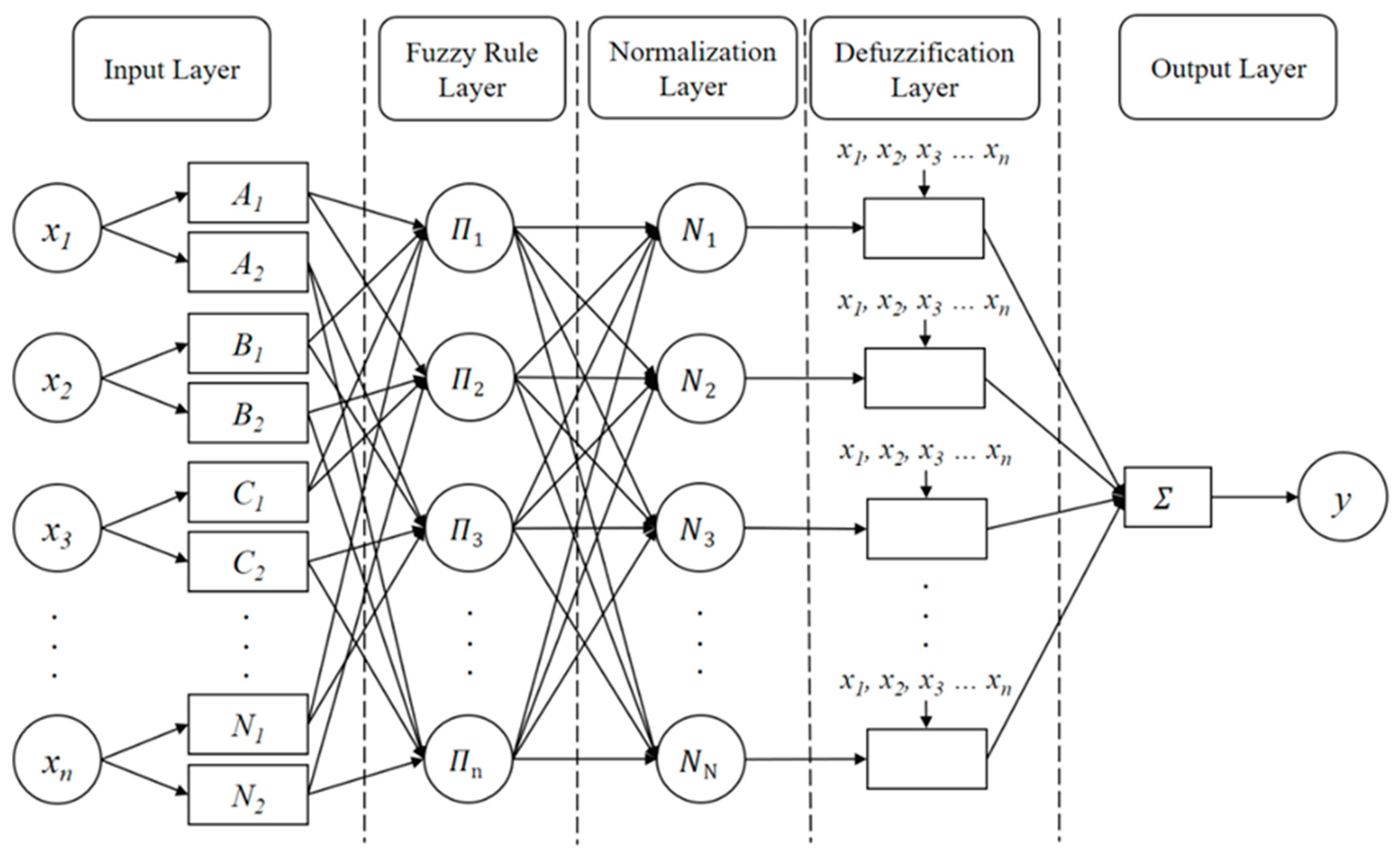
4.2. ANFIS Typhoon Intensity Forecast Model Construction

In ANFIS architecture, the main optimized parameters are nonlinear premise parameters ($c_{ji},{\sigma }_{ji}$) as presented in Equation (3), and the linear conclusion parameter is presented in Equation (6). The hybrid learning rule [21] used in this study optimized linear and nonlinear parameters separately. The least-square estimator optimized parameters in the linear parameter set, and the steepest gradient descent method optimized the nonlinear parameter set. This compound structure can effectively search for model parameters and improve the speed of model convergence. In the ANFIS model construction process, the radius of influence of SC was first determined. An initial FIS architecture was built after obtaining clustering results. Then, the training data were input into the FIS architecture to solve the linear and nonlinear parameter sets. Finally, the model was trained until the convergence.

This study used MI as the basis for ANFIS model selection to avoid overfitting and underfitting. The ANFIS data used were divided into ANFIS_SHIPSa and ANFIS_SHIPSb. The process of selecting the optimal ANFIS is shown in Figure 3. A different radius of influence was tested in order to build multiple ANFIS sets to finally obtain the model with the lowest MI as the ANFIS typhoon intensity forecast model network.

Table 6. Influence radius and rule number for establishing ANFIS models.

	ANFIS_SHIPSa			ANFIS_SHIPSb
Lead Time (h)	MI (kts)	Range of Influence	Rule No.	MI (kts)	Range of Influence	Rule No.
12	0.98	0.87	2	1.00	0.74	4
24	1.00	0.67	2	2.01	0.62	5
36	2.95	0.95	3	2.73	0.93	5
48	3.37	0.79	4	3.18	0.73	7
60	2.08	0.80	2	2.52	0.91	2
72	1.96	0.68	2	1.86	0.66	3
84	1.33	0.80	2	0.96	0.78	3
96	0.90	0.78	3	0.90	0.78	4
108	1.77	0.95	3	2.32	0.85	4
120	0.61	0.82	3	1.24	0.93	3

shows MI, radius of influence, and the number of rules of ANFIS typhoon intensity forecast models for 12 to 120 h.

4.3. MLR Typhoon Intensity Forecast Baseline Model Construction

To evaluate the improvement of the ANFIS on the typhoon intensity forecast by the MLR method, two additional MLR models were built in this study as baseline models for comparison. In the baseline models, all predictors of ANFIS were used, and MLR was used to forecast DELV. Unlike ANFIS, which uses three sets of data (training, validation, and testing data), MLR requires only two sets of data, one for training and one for testing. In the MLR baseline model, data from 2000 to 2005 were used as training data (same as ANFIS), and data from 2009 to 2012 were used as testing data.

In this study, the multiple regression coefficients of MLR were obtained from training data. Then predictive variables of testing data from 2009 to 2012 were used to obtain the multiple regression coefficients of training data to forecast DELV. Finally, two MLR baseline models, MLR_SHIPSa and MLR_SHIPSb, were built.

5. Results

5.1. Model Error and Underestimated Ratio

This study used improvement percentages of RMSE and underestimated ratios as evaluation indicators. Figure 4 shows the improvement percentage of RMSE when comparing the ANFIS typhoon forecast model with the MLR model. The improvement showed a decreasing trend from 96 h onwards. The difference in the improvement percentage of RMSE between models built with SHIPSa and SHIPSb was about 1%. The performance of models built for 84 h before the lead time with ANFIS and SHIPSb was improved. The performance of models built for 96 h after the lead time with ANFIS and SHIPSb was also improved.

JTWC Northwest Pacific typhoon intensity grade division standard was used in this study. The grade standard categorizes wind speeds greater than 130 kts as super typhoons and wind speeds between 63 kts and 129 kts as standard typhoons. The observed values of testing data and predicted values of various models were classified to evaluate the improvement percentage of the underestimated ratio of ANFIS. Figure 5 shows the improvement percentage of the underestimated ratio of ANFIS under different JTWC typhoon intensity standards. Figure 5a shows that in the case of standard typhoons, the underestimated ratio of ANFIS_SHIPSb was improved but was insignificant when compared with that of ANFIS_SHIPSa. Figure 5b shows the improvement percentage of the underestimated ratio of ANFIS under super typhoon intensity. It can be seen from the figure that the two models slightly increased the underestimated ratios for the super typhoon forecast.

5.2. Case Forecast Performance Evaluation

In this study, 2011’s Typhoon Songda was taken as an example for performance comparison. The number JTWC given Typhoon Songda was WP042011, and the warning time was from 12 p.m. on 20 May 2011 to 12 p.m. on 29 May 2011. Due to the utilization of the SHIPS dataset from 2000 to 2012, Typhoon Songda exhibited significant intensity variations and experienced RI multiple times. This study did not specifically investigate the features of RI; it only discussed the performance of the ANFIS typhoon intensity forecast model tested on the Typhoon Songda. The track and intensity of Typhoon Songda are shown in Figure 6.

Based on ANFIS_SHIPSa and ANFIS_SHIPSb, the bias, average bias, and maximum bias between the predicted and observed values of Typhoon Songda were calculated. Then, the improvement of the two models over the performance of the MLR model was analyzed. Figure 7 shows the improvement percentage of average bias and maximum bias of ANFIS_SHIPSa and ANFIS_SHIPSb (the corresponding mean and maximum bias of MLR are shown in

Table 7. Improvement percentage of mean bias and maximal bias in ANFIS model for Typhoon Songda.

Lead Time (h)	MLR_SHIPSa		MLR_SHIPSb
	Mean Bias (kt)	Maximum Bias (kt)	Mean Bias (kt)	Maximum Bias (kt)
12	−1.57	9.9	−1.31	9.79
24	−3.07	13.38	−2.55	13.52
36	−2.99	15.18	−3.74	15.49
48	−4.66	23.9	−5.42	24.34
60	−7.52	37.27	−8.48	32.03
72	−11.07	37.2	−11.01	38.18
84	−15.09	49.8	−15.55	49.05
96	−22.51	44.34	−22.51	44.34
108	−29.67	33.06	−30.53	29.32
120	−35.78	33.38	−34.47	34.17

) in the intensity forecast of Typhoon Songda, compared with the MLR model. In the figure, the circle shows the improvement of ANFIS_SHIPSa on MLR_SHIPSa. The cross shows the improvement of ANFIS_SHIPSb on MLR_SHIPSb. The dotted and solid lines are the improvement percentage of average bias and maximum bias, respectively. The figure also shows that the improvement of average bias gradually increased 60 h before the lead time. The improvement percentage of average bias was the largest at 48 h lead time. The improvement of average bias decreased 60 h after the lead time but was still positive. For the improvement of maximum bias of the two models, the improvement at 84 h lead time was the highest, at about 40%.

6. Conclusions

This section is not mandatory but can be added to the manuscript if the discussion is unusually long or complex.

• The radius of influence in various forecast models were determined by the MI indicator selection method and could effectively obtain small MAE difference between training and validation data. The MI indicator selection method could successfully select the ranges of influence and improve the testing performance of models.
• With the inclusion of the oceanic factors selected by SRP, except that the result of the 96-h lead time forecast model, was the same as that of the model only using atmospheric combinations, the oceanic factors were all added to the input variables in other forecast models. RHCN (ocean heat content) was selected in the 12~60 h forecast, and RSST (surface sea temperature) had the greatest influence in the 60~120 h forecast.
• In terms of RMSE improvement, both ANFIS_SHIPSa and ANFIS_SHIPSb demonstrate similar improvement trends compared to the MLR forecasts, with improvements ranging from approximately 1% to 8%. Among them, the ANFIS model at a lead time of 84 h exhibits the best improvement performance.
• ANFIS_SHIPSa and ANFIS_SHIPSb positively improved the average bias of the MLR model in the intensity forecast of Typhoon Songda. The improvement percentage of average bias of ANFIS_SHIPSa was the highest (125%) at 48 h lead time. The improvement percentage of average bias of ANFIS_SHIPSb was the highest (108%) at 36 h lead time. The maximum bias of ANFIS_SHIPSa was greatly improved at 60 h of the lead time, and the improvement percentage of maximum bias was the highest (39%) at 84 h of lead time. The maximum bias of ANFIS_SHIPSb was improved the most at 84 h lead time, with an improvement percentage of 43%.
• Overall, ANFIS could effectively improve the performance of MLR in typhoon intensity forecast. The model considering both atmospheric and oceanic environmental factors outperformed the models only considering the atmospheric environmental factor in typhoon intensity forecast.

7. Limitations and Future Work

The methods proposed in this study did not consider the characteristics of RI of typhoons. Future development will focus on further developing in this direction.

References

1. DeMaria, M.; Mainelli, M.; Shay, L.K.; Knaff, J.A.; Kaplan, J. Further Improvements to the Statistical Hurricane Intensity Prediction Scheme (SHIPS). Weather Forecast. 2005, 20, 531–543. [Google Scholar] [CrossRef] [Green Version]
2. DeMaria, M.; Sampson, C.R.; Knaff, J.A.; Musgrave, K.D. Is Tropical Cyclone Intensity Guidance Improving? Bull. Am. Meteorol. Soc. 2014, 95, 387–398. [Google Scholar] [CrossRef] [Green Version]
3. Jarvinen, B.R.; Neumann, C.J. Statistical Forecasts of Tropical Cyclone Intensity for the North Atlantic Basin. NOAA Technical Memorandum NWS NHC-10. 1979. Available online: https://repository.library.noaa.gov/view/noaa/6555 (accessed on 31 July 2023).
4. Chang, L.-C.; Chang, F.-J.; Yang, S.-N.; Tsai, F.-H.; Chang, T.-H.; Herricks, E.E. Self-organizing maps of typhoon tracks allow for flood forecasts up to two days in advance. Nat. Commun. 2020, 11, 1983. [Google Scholar] [CrossRef] [Green Version]
5. Jiang, S.; Fan, H.; Wang, C. Improvement of Typhoon Intensity Forecasting by Using a Novel Spatio-Temporal Deep Learning Model. Remote Sens. 2022, 14, 5205. [Google Scholar] [CrossRef]
6. Knaff, J.A.; DeMaria, M.; Sampson, C.R.; Gross, J.M. Statistical, 5-Day Tropical Cyclone Intensity Forecasts Derived from Climatology and Persistence. Weather Forecast. 2003, 18, 80–92. [Google Scholar] [CrossRef]
7. Ruttgers, M.; Jeon, S.; Lee, S.; You, D. Prediction of Typhoon Track and Intensity Using a Generative Adversarial Network With Observational and Meteorological Data. IEEE Access 2022, 10, 48434–48446. [Google Scholar] [CrossRef]
8. Xu, G.; Lin, K.; Li, X.; Ye, Y. SAF-Net: A spatio-temporal deep learning method for typhoon intensity prediction. Pattern Recognit. Lett. 2022, 155, 121–127. [Google Scholar] [CrossRef]
9. Yuan, S.; Wang, C.; Mu, B.; Zhou, F.; Duan, W. Typhoon Intensity Forecasting Based on LSTM Using the Rolling Forecast Method. Algorithms 2021, 14, 83. [Google Scholar] [CrossRef]
10. Knaff, J.A.; Sampson, C.R.; DeMaria, M. An Operational Statistical Typhoon Intensity Prediction Scheme for the Western North Pacific. Weather Forecast. 2005, 20, 688–699. [Google Scholar] [CrossRef] [Green Version]
11. Sharma, N.; Ali, M.M.; Knaff, J.A.; Chand, P. A soft-computing cyclone intensity prediction scheme for the Western North Pacific Ocean. Atmos. Sci. Lett. 2013, 14, 187–192. [Google Scholar] [CrossRef]
12. Sandhya, N.; Charanjeet, K.R. A review on machine learning techniques. Int. J. Recent Innov. Trends Comput. Commun. 2016, 4, 451–458. [Google Scholar]
13. Lin, S.S.; Tsai, H.C.; Kan, B.S.; Liao, Y.P. Integrating clustering analysis and artificial intelligence for typhoon hourly rainfall forecast. Taiwan Water Conserv. 2009, 57, 89–104. [Google Scholar]
14. Li, C.-Y.; Lin, S.S.; Lin, Y.F.; Kan, P.S. A bootstrap regional model for assessing the long-term impacts of climate change on river discharge. Int. J. Hydrol. Sci. Technol. 2019, 9, 84. [Google Scholar] [CrossRef]
15. Mulia, I.E.; Tay, H.; Roopsekhar, K.; Tkalich, P. Hybrid ANN–GA model for predicting turbidity and chlorophyll-a concentrations. J. Hydro-Environ. Res. 2013, 7, 279–299. [Google Scholar] [CrossRef]
16. Samsudin, R.; Saad, P.; Shabri, A. A hybrid least squares support vector machines and GMDH approach for river flow forecasting. Hydrol. Earth Syst. Sci. Discuss. 2010, 7, 3691–3731. [Google Scholar] [CrossRef]
17. Swain, D.; Ali, M.M.; Weller, R.A. Estimation of mixed-layer depth from surface parameters. J. Mar. Res. 2006, 64, 745–758. [Google Scholar] [CrossRef] [Green Version]
18. Jin, L.; Yao, C.; Huang, X.-Y. A Nonlinear Artificial Intelligence Ensemble Prediction Model for Typhoon Intensity. Mon. Weather Rev. 2008, 136, 4541–4554. [Google Scholar] [CrossRef]
19. Alvisi, S.; Franchini, M. Fuzzy neural networks for water level and discharge forecasting with uncertainty. Environ. Model. Softw. 2011, 26, 523–537. [Google Scholar] [CrossRef]
20. El-Shafie, A.; Jaafer, O.; Seyed, A. Adaptive neuro-fuzzy inference system based model for rainfall forecasting in Klang River, Malaysia. Int. J. Phys. Sci. 2011, 6, 2875–2888. [Google Scholar] [CrossRef]
21. Jang, J.-S.R. ANFIS: Adaptive-Network-Based Fuzzy Inference System. IEEE Trans. Syst. Man Cybern. 1993, 23, 665–685. [Google Scholar] [CrossRef]
22. Chang, F.-J.; Chiang, Y.-M.; Tsai, M.-J.; Shieh, M.-C.; Hsu, K.-L.; Sorooshian, S. Watershed rainfall forecasting using neuro-fuzzy networks with the assimilation of multi-sensor information. J. Hydrol. 2014, 508, 374–384. [Google Scholar] [CrossRef] [Green Version]
23. Chang, F.-J.; Chung, C.-H.; Chen, P.-A.; Liu, C.-W.; Coynel, A.; Vachaud, G. Assessment of arsenic concentration in stream water using neuro fuzzy networks with factor analysis. Sci. Total Environ. 2014, 494–495, 202–210. [Google Scholar] [CrossRef]
24. Chang, F.-J.; Lai, H.-C. Adaptive neuro-fuzzy inference system for the prediction of monthly shoreline changes in northeastern Taiwan. Ocean Eng. 2014, 84, 145–156. [Google Scholar] [CrossRef]
25. Nayak, P.C.; Sudheer, K.P.; Rangan, D.M.; Ramasastri, K.S. A neuro-fuzzy computing technique for modeling hydrological time series. J. Hydrol. 2004, 291, 52–66. [Google Scholar] [CrossRef]
26. Chiu, S.L. Fuzzy Model Identification Based on Cluster Estimation. J. Intell. Fuzzy Syst. 1994, 2, 267–278. [Google Scholar] [CrossRef]
27. Fattahi, H. Indirect estimation of deformation modulus of an in situ rock mass: An ANFIS model based on grid partitioning, fuzzy c-means clustering and subtractive clustering. Geosci. J. 2016, 20, 681–690. [Google Scholar] [CrossRef]
28. Talpur, N.; Salleh, M.N.M.; Hussain, K. An investigation of membership functions on performance of ANFIS for solving classification problems. In IOP Conference Series: Materials Science and Engineering; IOP Publishing: Bristol, UK, 2017; Volume 226, p. 012103. [Google Scholar]
29. Chang, L.-C.; Chang, F.-J. Intelligent control for modelling of real-time reservoir operation. Hydrol. Process. 2001, 15, 1621–1634. [Google Scholar] [CrossRef]
30. DeMaria, M.; Kaplan, J. An Updated Statistical Hurricane Intensity Prediction Scheme (SHIPS) for the Atlantic and Eastern North Pacific Basins. Weather Forecast. 1999, 14, 326–337. [Google Scholar] [CrossRef]
31. Lin, S.Y. Improvement of the Statistical Typhoon Intensity Prediction Model by Using the SHIPS Developmental Data. Unpublished Master’s Thesis, Tamkang University, New Taipei, Taiwan, 2016. [Google Scholar] [CrossRef]
Figure 1. ANFIS architecture (with N-dimensional input and one dimension output).
Water 15 02855 g001
Figure 2. Selected typhoon path map.
Water 15 02855 g002
Figure 3. Procedure for determining the best ANFIS model.
Water 15 02855 g003
Figure 4. Improvement percentage of RMSE of ANFIS compared to MLR.
Water 15 02855 g004
Figure 5. Improvement percentage of ANFIS compared to MLR in the underestimation ratio of JTWC typhoon standard and super typhoon forecast. (a) In the classification of typhoon intensity. (b) In the classification of super typhoon intensity.
Water 15 02855 g005
Figure 6. The relationship between the path of Typhoon Songda and the intensity of the typhoon through time.
Water 15 02855 g006
Figure 7. Improvement percentage of mean bias and maximal bias in ANFIS model for Typhoon Songda.
Water 15 02855 g007