Parameterization for Modeling Blue–Green Infrastructures in Urban Settings Using SWMM-UrbanEVA

Abstract

Blue–green infrastructures (BGI) play an important role in addressing contemporary challenges posed by urbanization, climate change, and demographic shifts. This study focuses on the parameterization of BGI within hydrological models, specifically emphasizing the Low Impact Development (LID) module of the Storm Water Management Model (SWMM), supplemented by the SWMM-UrbanEVA evapotranspiration model. Employing a systematic approach, a transferable framework is developed to categorize BGI types, leading to a comprehensive parameterization toolset. This toolset includes parameter estimates for predefined BGI types, encompassing both natural and technical systems with a specific emphasis on plant-specific parameterization. The justification of these parameter estimates is supported by an extensive literature review. Sensitivity analyses reveal the influence of plant-specific parameters, such as the crop factor (K_C), and soil storage capacity, on water balance and peak runoff. Additionally, this study presents practical guidelines to enhance the comprehension of model behavior and ensure the highest possible quality in model parameterization. While further research on validity and transferability of the toolset is required, the findings of this study provide useful support for the differentiated representation and analysis of hydrological processes in urban environments. As a result, this study serves as a valuable resource for researchers, practitioners, and decision makers, facilitating the implementation of sustainable water management practices in urban settings.

1. Introduction

Urbanization, climate change, and demographic shifts pose increasing challenges to cities. Extensive urban land sealing, in particular, impacts the water and energy balance, resulting in reduced groundwater recharge and evapotranspiration (ET) and increased runoff volume and peaks [1]. Moreover, ET reduction directly influences the urban climate [2], contributing to higher temperatures in urban areas (urban heat islands [3]). Addressing these challenges requires solutions, such as blue–green infrastructure (BGI), to ensure resilient water management in urban environments. Previous studies have examined water quality and quantity (e.g., [4,5,6]) as well as cooling effects associated with BGIs (e.g., [7,8,9]). Other studies also highlight additional benefits such as increased biodiversity and improved livability [10,11,12].

For decision making regarding the integration of BGI into water management and urban planning purposes, it is important to gain a further understanding of the impact of BGI on the overall hydrologic regime. Precise and long-term analysis of the temporal dynamics of water balance components is essential [13,14]. Investigations should examine (i) the behavior of BGI during precipitation events and (ii) dry periods, and (iii) their interactions and (iv) impacts on the existing sewer system [15,16]. They can be carried out using either measurement or modeling approaches. While measurements can provide insights into existing conditions, they can be resource and cost intensive to maintain. Conversely, models offer the advantage of simulating various scenarios, making them flexible tools for studying BGI.

In hydrological studies of BGI in urban areas, it is crucial to consider the representation of the plant–soil–atmosphere system [17,18,19,20]. Physically-based models, such as “Soil-Water-Atmosphere-Plant” (SWAP) [21], “Water balance Simulation Model” (WaSiM) [22] or HYDRUS-1D [23], often use globally recognized reference grass evapotranspiration ET₀ and plant-specific crop factor K_C by Allen et al. [24]. To further capture the dynamics of plant-specific evapotranspiration, they incorporate approaches, like soil covered fraction [21,25,26,27] and water-wetted leaf area [28,29]. This is achieved through the characterization of plant-specific parameters, including the leaf area index (LAI), leaf storage coefficient, and interception capacity [21,23,30,31,32]. Soil dynamics are often characterized by Richards equation [33]. However, physically-based models are computationally intensive and challenging to parameterize due to the large number of parameters required and associated parameter uncertainties [34]. Therefore, their application for modeling urban settings with numerous heterogeneous surfaces is not effective. In contrast, simple empirical alternatives were employed but fell short in accurately representing the plant–soil–atmosphere system. They neglect the influence of available soil water or do not account for plant-specific characteristics, such as their temporal and local variability [20,35,36].

One widely used rainfall–runoff model is the Storm Water Management Model (SWMM) developed by the US Environmental Protection Agency (EPA) [37]. It includes a module called Low Impact Development (LID) that allows the simulation of various BGIs and other stormwater management measures such as permeable pavements and rainwater harvesting [38]. Several studies have addressed the shortcomings of oversimplified modeling of ET processes in SWMM-LID modules [17,39,40]. Therefore, SWMM-UrbanEVA was developed to address the existing deficiencies in modeling urban BGI evapotranspiration [41]. The fully integrated submodel complements SWMM by enabling the plant-specific modeling of evapotranspiration for BGIs. It has undergone validation for simulating the water balance of different BGIs [41,42,43], but further investigations are required for parameterization.

On the one hand, previous research has indicated a high sensitivity of the water balance to plant-specific parameters such as the crop factor K_C and leaf area index LAI. However, knowledge of K_C for urban vegetation remains limited, as the crop factor approach originally goes back to agricultural irrigation management [24]. On the other hand, numerous studies have applied or further examined parameterization of existing SWMM-LID module. These studies typically focus on specific LID systems and differ in their investigation’s focus, including sensitivity analyses (e.g., [44]), model calibration, and validation against measurements (e.g., [18,45]), or the simple application of recommended parameterization estimates (e.g., [46,47]). However, there is a lack of systematic documentation regarding the applied parameterizations and the investigation of sensitivities, uncertainties, and validity. Due to the increasing relevance of BGI in the urban context and the accompanying more frequent mapping in hydrological models such as SWMM, it is essential to compile and organize this information to enhance understanding and ensure robustness in future applications of the SWMM-LID module. Furthermore, the addition of plant-specific parameterization is important for accurate mapping of BGI.

Therefore, this study focuses on the systematic preparation of BGI model parameterization in order to develop a reliable basis for further application and validation of modeling BGI in urban settings. A transferable toolset should be developed focusing on SWMM-LID parameterization supplemented by SWMM-UrbanEVA. The development contains the following topics:

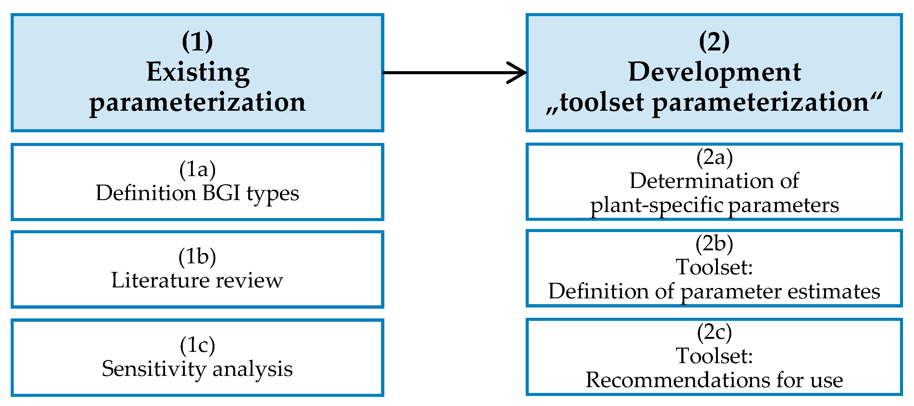
• Transferable definition of BGI types: The study aims to define BGI types that will enable the accurate representation of different BGI features and their associated parameters in the model.
• Structured analysis of parameter sensitivities: The study will conduct a systematic analysis of the sensitivity of model inputs to key outputs. By identifying the most influential parameters, users can prioritize their parameterization efforts and improve the overall accuracy of the model.
• Parameter estimates: Based on a comprehensive literature review, the study will offer structured and comprehensive recommendations for parameterizing the LID module in SWMM, including parameter estimates and ranges.
• Recommendations for use: The study will provide practical guidelines and recommendations for effectively parameterizing SWMM-UrbanEVA.

2. Materials and Methods

2.1. Study Design

The study was conducted in three steps, as illustrated in Figure 1. The first step involved an analysis of existing parameterization. Firstly, BGI types were defined by comparing the model structure with relevant BGI structures (Step 1a). Additionally, a literature review was conducted to examine the parameterization of existing SWMM-LID-modules (Step 1b). Furthermore, a sensitivity analysis was performed to assess the correlation of model inputs and outputs (Step 1c).

The second step focused on the development of a transferable parameter toolset. Firstly, plant-specific parameters of SWMM-UrbanEVA were determined (Step 2a). This was followed by the definition of parameter estimates, derived from the findings of points 1b, 1c, and 2a (Step 2b). Finally, recommendations for using the toolset were established to ensure robust model parameterization (Step 2c).

2.2. Model Description

The Stormwater Management Model (SWMM) [48], developed by the US EPA, is a dynamic rainfall–runoff model. It simulates various hydrologic processes, including surface hydrology and runoff routing in sewer systems. Its comprehensive framework aids in analyzing urban stormwater systems and supports decision making. The model includes an LID module (Low Impact Development) for modeling various BGI systems such as green roofs, rain gardens, permeable pavements, and rainwater harvesting systems [38].

The SWMM-LID module incorporates a horizontal three-layer system consisting of a surface layer, a soil layer, and a storage layer. The surface layer is responsible for generating runoff and facilitating infiltration into the underlying soil layer. Depending on the BGI system, the surface layer represents natural depressions or technically constructed retention volumes, including variations in vegetation type, slope, and ponding depth. The soil layer enables modeling percolation, retention, and evapotranspiration processes depending on soil moisture. In reality, it may be natural soil or engineered substrate. The storage layer provides further retention space prior to infiltration into the native soil. It can be constructed of porous soils (e.g., gravel) or engineered trench systems, providing the option of sealing the system down to the natural soil. The addition of a drainage layer (e.g., drainage mat, conventional drain pipe) is optional [38].

The complementary submodel SWMM-UrbanEVA [41] addresses previous limitations of the highly simplified evapotranspiration modeling in SWMM by integrating time-, location-, and plant-dependent model approaches. Therefore, it is particularly suitable for modeling BGI.

SWMM-UrbanEVA incorporates two subprocess models (SM). SM 1 considers the reduction in potential evapotranspiration due to shading effects from surrounding buildings or extensive vegetation. SM 2 includes an evapotranspiration approach for vegetated areas to consistently represent various BGI. The three-layer system of the SWMM LID-module (surface–soil–storage) is retained and extended with a new vegetation layer (Figure 2). The local potential evapotranspiration ET_0,Ks can be adjusted to the existing vegetation using the crop factor K_C.

Since this study focuses on the application and parameterization of the SM2, no mitigation of ET₀ by shading will be applied in the following (ET_0,Ks = ET₀). Thus, SM1 will not be considered further.

Further information on SWMM-UrbanEVA including a detailed model description can be found in [41].

2.3. Investigations on Existing Parameterization

2.3.1. Definition of Investigated of BGI Types

The sought definition of BGI types must be transferable and flexible, allowing for the representation of different systems. It is limited to vegetated and open-air structures, as SWMM-UrbanEVA focuses on plant-related evapotranspiration. Distinctions need to be made between: (i) technical and natural systems, (ii) systems with and without groundwater recharge, (iii) systems with and without storage layers, and (iv) systems with and without underdrain.

The classification based on these requirements is illustrated structurally in Figure 3.

Table 1. Definition of investigated BGI types including an overview of integrated system elements and investigated model output fluxes.

	BGI Type	Definition	System Elements 1					Model Output Fluxes 2
			Su	So	St	St-seal	Dr	R-O	R-D	E	I
2-LAYER	01_2L-IB	2-layer system, (i) technical infiltration systems, not providing an additional storage layer, or (ii) natural systems	✓	✓				✓		✓	✓
3-LAYER	02_3L-BC	technical 3-layer system, bioretention cells and structurally similar systems, summarizes types 2a–2c, if infiltration as well as underdrain are not further specified	✓	✓	✓	(✓)	(✓)	✓	(✓)	✓	(✓)
	02a_3L-BC- infil	technical 3-layer system, bioretention cells and structurally similar systems, providing infiltration, no underdrain	✓	✓	✓			✓		✓	✓
	02b_3L-BC-drain	technical 3-layer system, bioretention cells and structurally similar systems, providing underdrain, no infiltration	✓	✓	✓	✓	✓	✓	✓	✓
	02c_3L-BC- dr-infil	technical 3-layer system, bioretention cells and structurally similar systems, providing infiltration and underdrain	✓	✓	✓		✓	✓	✓	✓	✓
	03_3L-GR	technical 3-layer system, green roofs (extensive or intensive systems, with increased retention capacities or as a roof garden), providing underdrain, no infiltration	✓	✓	✓	✓	✓	✓	✓	✓

Note: ¹ integrated system elements: Su = surface layer; So = soil layer; St = storage layer; St-seal = sealing to natural soil; Dr = underdrain; ² investigated model output fluxes: R-O = runoff (overflow); R-D = runoff (drain); E = evapotranspiration; I = infiltration into natural soil.

adds the associated definitions as well as an overview of system elements and model output fluxes. A differentiation is made between 2-layer and 3-layer systems on the top level (Figure 3). The 2-layer systems represent (i) infiltration systems, not providing an additional storage layer, and (ii) natural systems. The systems consist of the vegetation layer along with the surface layer and the soil layer. The water percolates through the soil zone before infiltrating into the native soil. The height of the surface layer defines additional detention volume. Since infiltration systems and natural systems do not differ structurally, they are considered together in the following (“01_2L_IB”).

Moving on to the 3-layer systems, these are defined as technical systems that consist of the surface layer, soil layer, and storage layer. They can be divided into the two main groups bioretention cells (“02_3L_BC”) and green roofs (“03_3L-GR”). On the one hand, the bioretention cell (BC) is a versatile system that can be configured in various ways. BCs are suitable when the native soil has poor permeability or when additional retention capacity is required [49]. Due to structural differences the following three subtypes are defined: (i) pure infiltration elements (“02a_3L_BC-infil”), (ii) systems, sealed to the native ground with underdrains (“02b_3L_BC-drain”), and (iii) a combination of infiltration and underdrain (“02c_3L_BC-dr-inf”). On the other hand, green roofs differ from BCs in terms of their construction height and substrate composition. They also follow a three-layer system configuration, consisting of a vegetation layer, surface layer, soil layer, and storage layer. Green roofs can be designed as extensive or intensive systems, with increased retention capacities or as a roof garden. Since those options do not differ structurally, they are considered together in the following (“03_3L-GR”).

2.3.2. Literature Review—SWMM-LID-Parameterization

An extensive exploration of the parameterization of SWMM-LID models found in the literature was conducted. Web of Science and Scopus were used as primary databases for the review. Studies published between 2013 and 2023 that contained “SWMM LID”, “SWMM low impact development”, “SWMM blue green infrastructure”, or “SWMM green infrastructure” in the title, abstract, or keywords were considered. Citing or cited studies that met the same criteria were added secondarily. Only studies that used the SWMM-LID module and presented a justified parametrization were collected. The reviewed parameter values had been selected by the authors based on (i) measurements, (ii) the actual design of the system, (iii) the literature, (iv) calibration processes, or (v) the authors’ own assumptions.

The studies employed either the preset SWMM-LID modules, namely (i) vegetative swale, (ii) green roof, (iii) rain garden, or (iv) bioretention cell. In other cases, the SWMM-LID module bioretention cell was used, being manually adjusted to all desired configurations. Nonvegetated elements, such as infiltration trenches, were not considered.

To establish a coherent classification, the systems mentioned in the literature were assigned to the predefined BGI types (Section 2.3.1). Considering the similar fundamental characteristics at surface, soil, and storage configuration of the three BC systems 02a–02c, the review only distinguished between the main BGI types infiltration basins (“01_2L_IB”), bioretention cells (“02_3L_BC”), and green roofs (“03_3L-GR”). The assignment of reviewed systems to the predefined BGI types was made depending on the functional system structure (e.g., use of SWMM layers/parameters, use of preset SWMM-LID modules). An overview is presented in

Table 2. Assignment of systems found in literature to predefined BGI types.

System	01_2L-IB	02_3L-BC	03_3L-GR
Vegetative swale	✓	✓
Infiltration swale	✓
Grass swale	✓
Swale		✓
Green belt	✓	✓
Rain garden	✓	✓
Bioretention cell		✓
Green roof			✓
Retention roof			✓

.

All reviewed parameter estimates were checked for plausibility before inclusion into the data set. The evaluation of the data was carried out typology- and parameter-wise. When the authors had used the preset SWMM-LID module “green roof”, the parameters depth of drainage mat and void fraction of drainage mat were interpreted as depth and void fraction of storage layer.

2.3.3. Sensitivity Analysis

To investigate the impact of parameter variations in previously defined BGI types on model outputs, a global sensitivity analysis was conducted. The predefined SWMM-LID-module “bioretention cell” was adjusted for the different BGI types. An overview of varied model parameters and their ranges can be found in Table 3. The ranges (columns “min” and “max”) were selected in accordance with parameter estimates given in the literature (column “Ref.”). Depending on the BGI type, not all parameters of the SWMM-bioretention cell were needed, hence some parameters were fixed. They are displayed in grey. For all simulations, K_S was set to 1. ET was only considered in dry phases. The analysis was performed for the model outputs runoff, infiltration, and evapotranspiration (in mm) as well as for LID peak runoff (in l·s⁻¹·ha⁻¹). Climate data (precipitation, temperature, wind speed, radiation, relative humidity), measured at the full scale lysimeter St. Arnold [50], were used for simulation with a length of 10 years (01.01.1989–01.01.1999). The lysimeter is located 30 km northwest of Münster, Germany, and has a long-term average of 460 mm ET₀ and 793 mm precipitation. ET₀ was calculated as model input on a daily timestep based on Allen et al. [24]. Precipitation was inserted with a 5 min timestep.

The KALIMOD software tool [51,52] was used for conducting the sensitivity analysis. KALIMOD serves as an interface between simulation models and parameter sampling as well as optimization algorithms. It imports SWMM and SWMM-UrbanEVA models, provides parameter sampling methods, manipulates the model files, and runs the simulations. Parameter sampling was conducted globally using Latin Hypercube Sampling (LHS) [53]. LHS is a statistical method for generating diverse and representative samples within specified ranges. By partitioning the parameter space into evenly spaced intervals, it ensures efficient exploration of the parameter range while minimizing redundancy. LHS allows for a reduction in model runs compared to Monte Carlo simulation using random samples [54]. The parameter sampling was performed following a uniform distribution. Following recommendations from Pianosi et al. [55], 100 simulations per parameter were executed.

To assess the relationship between the model parameters and the resulting outputs, the Pearson correlation coefficient (cor) [56] was adopted as the evaluation metric.

$$\mathrm{c}\mathrm{o}\mathrm{r}=\frac{\mathrm{c}\mathrm{o}\mathrm{v}(\mathrm{X},\mathrm{Y})}{{\mathsf{\sigma }}_{\mathrm{X}}{\mathsf{\sigma }}_{\mathrm{Y}}}$$

(1)

In which cov is the covariance, σ_x is the standard deviation of X, and σ_y is the standard deviation of Y. cor can take values between −1 and +1 where ±1 indicates direct correlation whereas 0 describes a missing correlation between two variables.

Table 3. Parameter ranges for sensitivity analysis. Abbreviations for BGI types are mentioned in Table 1. Parameters for sensitivity analysis are indicated as follows: black = varied parameter, grey = fixed parameter.

	Parameter		Unit	01_2L-IB			02_3L-BC			03_3L-GR
				Min	Max	Ref.	Min	Max	Ref.	Min	Max	Ref.
vegetation	crop factor	Veg_cf	-	0.5	2	[24]	0.5	2	[24]	0.5	2	[24]
	leaf area index	Veg_LAI	m2·m−2	1	16	[57]	1	16	[57]	1	16	[57]
	leaf storage coefficient	Veg_sl	-	0.05	1	[41]	0.05	1	[41]	0.05	1	[41]
	aWC-threshold	Veg_aWCth	-	0.05	1	[41]	0.05	1	[41]	0.05	1	[41]
surface	surface storage	Su_Depth	mm	0	300	[38]	0	300	[38]	1	80	[38]
	surface roughness	Su_ManN	s·m−1/3	0.001	0.8	[58]	0.001	0.8	[58]	0.001	0.8	[58]
	surface slope	Su_Slope	%	0	10	assum. 1	0	10	assum. 1	0	45	[59]
soil	soil depth	So_Depth	mm	0	1000	[49]	0	1300	[38]	30	300	[59]
	porosity	So_Por	-	0.25	0.65	[60]	0.25	0.65	[60]	0.25	0.65	[60]
	field capacity	So_FC	-	0.15	0.245	[60]	0.15	0.245	[60]	0.15	0.245	[60]
	wilting point	So_WP	-	0	0.145	[60]	0	0.145	[60]	0	0.145	[60]
	conductivity	So_Cond	mm·h−1	50	140	[38]	50	140	[38]	50	360	[59]
	conductivity slope	So_CondSl	-	30	55	[38]	30	55	[38]	30	55	[38]
	suction head	So_SucH	mm	50	100	[38]	50	100	[38]	50	100	[38]
storage	storage height	St_Depth	mm	0			0	1000	[38]	10	50	[38]
	void ratio	St_VoidR	-	0			0.2	0.4	[38]	0.2	0.4	[38]
	seepage rate	St_SeepR	mm·h−1	18	360	[49]	3.6 2,4	72 2,4	[49]	0
							0 3
underdrain	drain coefficient	UD_Coeff	mm·h−1	0			0.1 3,4	100 3,4	assum. 1	0.1	100	assum. 1
							0 2
	drain exponent	UD_Exp	-	0			0.1 3,4	1 3,4	assum. 1	0.1	1	assum. 1
							0 1
	offset	UD_OffS	mm	0			0 3,4	500 3,4	assum. 1	0	50	assum. 1
							0 1

Note: ¹ assumption; ² 02a_3L-BC-infil; ³ 02b_3L-BC-drain; ⁴ 02c_3L-BC-inf-dr.

Table 3. Parameter ranges for sensitivity analysis. Abbreviations for BGI types are mentioned in Table 1. Parameters for sensitivity analysis are indicated as follows: black = varied parameter, grey = fixed parameter.

	Parameter		Unit	01_2L-IB			02_3L-BC			03_3L-GR
				Min	Max	Ref.	Min	Max	Ref.	Min	Max	Ref.
vegetation	crop factor	Veg_cf	-	0.5	2	[24]	0.5	2	[24]	0.5	2	[24]
	leaf area index	Veg_LAI	m2·m−2	1	16	[57]	1	16	[57]	1	16	[57]
	leaf storage coefficient	Veg_sl	-	0.05	1	[41]	0.05	1	[41]	0.05	1	[41]
	aWC-threshold	Veg_aWCth	-	0.05	1	[41]	0.05	1	[41]	0.05	1	[41]
surface	surface storage	Su_Depth	mm	0	300	[38]	0	300	[38]	1	80	[38]
	surface roughness	Su_ManN	s·m−1/3	0.001	0.8	[58]	0.001	0.8	[58]	0.001	0.8	[58]
	surface slope	Su_Slope	%	0	10	assum. 1	0	10	assum. 1	0	45	[59]
soil	soil depth	So_Depth	mm	0	1000	[49]	0	1300	[38]	30	300	[59]
	porosity	So_Por	-	0.25	0.65	[60]	0.25	0.65	[60]	0.25	0.65	[60]
	field capacity	So_FC	-	0.15	0.245	[60]	0.15	0.245	[60]	0.15	0.245	[60]
	wilting point	So_WP	-	0	0.145	[60]	0	0.145	[60]	0	0.145	[60]
	conductivity	So_Cond	mm·h−1	50	140	[38]	50	140	[38]	50	360	[59]
	conductivity slope	So_CondSl	-	30	55	[38]	30	55	[38]	30	55	[38]
	suction head	So_SucH	mm	50	100	[38]	50	100	[38]	50	100	[38]
storage	storage height	St_Depth	mm	0			0	1000	[38]	10	50	[38]
	void ratio	St_VoidR	-	0			0.2	0.4	[38]	0.2	0.4	[38]
	seepage rate	St_SeepR	mm·h−1	18	360	[49]	3.6 2,4	72 2,4	[49]	0
							0 3
underdrain	drain coefficient	UD_Coeff	mm·h−1	0			0.1 3,4	100 3,4	assum. 1	0.1	100	assum. 1
							0 2
	drain exponent	UD_Exp	-	0			0.1 3,4	1 3,4	assum. 1	0.1	1	assum. 1
							0 1
	offset	UD_OffS	mm	0			0 3,4	500 3,4	assum. 1	0	50	assum. 1
							0 1

Note: ¹ assumption; ² 02a_3L-BC-infil; ³ 02b_3L-BC-drain; ⁴ 02c_3L-BC-inf-dr.

2.4. Development “Toolset Parameterization”

Determination of Plant-Specific Parameters

Various plant-specific parameters are addressed in evapotranspiration modeling. Focusing on SWMM-UrbanEVA here, a comprehensive description of the model can be found in Hörnschemeyer et al. [41]. For a concise overview of the plant-related parameters, please refer to Appendix A. Previous studies have highlighted K_C and LAI as the most influential parameters affecting the water balance in SWMM-UrbanEVA [41,43]. To enhance the applicability of parameter estimates, a good overview on K_C and LAI values for typical urban vegetation is missing.

The growth factor gf (Equation (A1), Appendix A) describes the vegetative LAI variation over the year. Building on the extensive work conducted by Bremicker [27] and Löpmeier [61], potential monthly gf values for use are provided in

Table A1. Exemplary growth factors gf (-) for different species.

No.	Type	Jan	Feb	Mar	Apr	May	Jun	Jul	Aug	Sep	Oct	Nov	Dec
1	grass 1	0.29	0.29	0.29	0.43	0.86	1.14	1.29	1.71	2.00	1.71	1.14	0.86
2	extensive green 2	0.68	0.68	0.68	1.01	1.18	1.35	1.35	1.35	1.18	1.01	0.85	0.68
3	intensive green 2	0.68	0.68	0.68	1.01	1.18	1.35	1.35	1.35	1.18	1.01	0.85	0.68
4	humid surfaces 2	0.55	0.55	0.83	1.10	1.38	1.38	1.38	1.38	1.38	0.83	0.69	0.55
5	coniferous 2	1.00	1.00	1.00	1.00	1.00	1.00	1.00	1.00	1.00	1.00	1.00	1.00
6	deciduous 2	0.09	0.09	0.26	0.69	1.21	1.90	2.07	2.07	1.90	1.38	0.26	0.09
7	vegetation general 3	0.35	0.35	0.43	0.66	1.08	1.70	1.81	1.85	1.70	1.13	0.54	0.40

Note: ¹ reference: [61]; ² reference: [27]; ³ evaluation of various species: [155].

(Appendix B) and will not be further discussed in the following. In contrast, LAI and K_C should be defined based on available literature. Thereby, the LAI could be determined directly from the literature. Due to limited knowledge regarding K_C values for plants in urban environments, K_C was calculated according to Allen et al. [24] using the Penman–Monteith equation for varying plant types.

$${\mathrm{K}}_{\mathrm{C}}=\frac{{\mathrm{E}\mathrm{T}}_{\mathrm{C}}}{{\mathrm{E}\mathrm{T}}_0}$$

(2)

ET_C is the crop evapotranspiration in mm·h⁻¹ under standard conditions and should be calculated using the Penman–Monteith equation [62] in the ASCE standardized format [63] (Equation (A3), Appendix A). ET_C was calculated varying the three key plant-specific parameters: LAI, crop height (H), and bulk stomatal resistance (g_s).

First, the following types of plants were considered as relevant: (i) trees (both deciduous and coniferous), (ii) woody plants up to a height of 2 m (e.g., hedges, large bushes), (iii) perennials and small shrubs, (iv) grasses and herbs, and (v) sedum and succulents. Whenever feasible, preference was given to climate-adapted species known for their resilience to drought and frost, considering the anticipated challenges posed by climate change. The selection of trees was guided by the climate species matrix [64] and the GALK (German Working Group for Landscaping and Environmental Planning) list on urban street trees [65]. Data regarding the remaining vegetation was sourced from [66,67,68,69]. The research identified 328 potentially relevant species. The complete list is available upon request.

Next, plant-specific parameters LAI, H, and g_s were derived from existing databases [57,70,71]. LAI was compiled in m² m⁻², H in m, and g_s in mm·s⁻¹. When g_s was published in mmol·m⁻²·s⁻¹ (e.g., [71]), values were divided by 41.57 for conversion, following Körner et al. [72] and assuming 293 K/20 °C and 101.3 kPa. In cases where the databases did not provide sufficiently reliable information, manually researched values, e.g., [73,74,75,76,77,78,79,80,81,82,83,84], were added. This was particularly necessary for sedum/succulents. In cases where the stomatal resistance r_l was published, g_s was determined as the reciprocal of r_l.

$${\mathrm{g}}_{\mathrm{s}}=\frac{1}{{\mathrm{r}}_{\mathrm{l}}}$$

(3)

The analysis was performed using the R scripting language. Duplicate analyses of the same source across multiple databases were excluded to ensure data integrity. Outliers were removed from the dataset using the 1.5 × IQR method. The Interquartile Range (IQR) was calculated as:

$$\mathrm{I}\mathrm{Q}\mathrm{R}=\mathrm{Q}3-\mathrm{Q}1$$

(4)

in which Q3 = third quartile and Q1 = first quartile.

The lower threshold for outliers was defined as:

$$\mathrm{L}\mathrm{o}\mathrm{w}\mathrm{e}\mathrm{r}\mathrm{T}\mathrm{h}\mathrm{r}\mathrm{e}\mathrm{s}\mathrm{h}\mathrm{o}\mathrm{l}\mathrm{d}=\mathrm{Q}1-1.5·\mathrm{I}\mathrm{Q}\mathrm{R}$$

(5)

and the upper threshold for outliers was defined as:

$$\mathrm{U}\mathrm{p}\mathrm{p}\mathrm{e}\mathrm{r}\mathrm{T}\mathrm{h}\mathrm{r}\mathrm{e}\mathrm{s}\mathrm{h}\mathrm{o}\mathrm{l}\mathrm{d}=\mathrm{Q}3+1.5·\mathrm{I}\mathrm{Q}\mathrm{R}$$

(6)

Data points falling below the lower threshold or above the upper threshold were considered outliers and subsequently removed from the dataset. This approach provided a systematic way to identify and handle outliers in the analysis.

To further investigate parameter uncertainties, the standard uncertainty $u\left(\overline{y}\right)$ was calculated according the “Guide to the Expression of Uncertainty in Measurement” (GUM [85,86]).

$$\mathrm{u}\left(\overline{\mathrm{y}}\right)=\frac{\mathrm{s}\left(\mathrm{y}\right)}{\sqrt{\mathrm{n}}}$$

(7)

in which y = measurement data; s(y) = standard deviation; and n = number of measurements.

Last, the calculation of K_C was conducted according to Equation (2) using mean values of previously determined parameters. The calculation was performed using climate data measured at the full scale lysimeter St. Arnold (Section 2.3.3). Combined standard uncertainties u_c were calculated for further uncertainty estimation.

$${{\mathrm{u}}_{\mathrm{c}}\left(\mathrm{y}\right)}^2=\sum _{\mathrm{i}=1}^{\mathrm{N}}{\mathrm{u}\left({\overline{\mathrm{y}}}_{\mathrm{i}}\right)}^2{\left(\frac{\partial {\mathrm{K}}_{\mathrm{C}}}{\partial {\overline{\mathrm{y}}}_{\mathrm{i}}}\right)}^2$$

(8)

3. Results

3.1. Investigations on Existing Parameterization

3.1.1. Literature Review—SWMM-LID-Parameterization

The literature review conducted for this study yielded insightful results, with a total of 132 entries sourced from 59 references. Twenty-four entries could be assigned to previous defined BGI type 01_2L-IB, 59 entries to 02_3L-BC, and forty-nine entries to 03_3L-GR (

Table 4. Number of BGI system entries found in literature assigned to predefined BGI types. Abbreviations for BGI types are mentioned in Table 1.

BGI System	01_2L-IB		02_3L-BC		03_3L-GR
	Count	References	Count	References	Count	References
Vegetative swale	12	[87,88,89,90,91,92,93,94,95,96,97]	1	[98]
Infiltration swale	1	[99]
Grass swale	1	[92]
Swale			1	[100]
Green belt	1	[95,101,102]	2	[101]
Rain garden	9	[46,47,87,90,103,104,105,106]	8	[101,107,108,109,110,111,112,113]
Bioretention cell			47	[45,47,87,88,92,93,94,96,98,99,104,109,114,115,116,117,118,119,120,121,122,123,124,125,126]
Green roof					48	[4,18,34,39,40,41,46,47,90,91,94,95,99,100,101,101,102,104,109,112,113,113,116,118,120,127,128,129,130,131,132,133]

). In the years 2013 to 2018, no more than one to five references were found annually. With seven to fifteen annual references, there has been a significant increase in the number of annual investigations since 2019 (Figure A1, Appendix C). Heterogeneous sources for parameter selection of reviewed entries could be detected, such as (i) measurements, (ii) the actual design of the system, (iii) the SWMM manual [38], (iv) the literature, (v) calibration processes, or (vi) the authors’ own assumptions (

Table A2. Sources for parameter selection found in the literature.

Source Type	Number of Parameter Estimates	%
measurement	109	7.7%
actual system design	144	10.1%
literature	430	30.2%
SWMM manual	234	16.5%
technical guideline	191	13.4%
calibration process	71	5.0%
author’s assumption	42	3.0%
no information	201	14.1%

, Appendix C). The majority of parameter selections were made on the basis of the literature (30%) or the SWMM manual (17%). Other sources were used in 3 to 13%. No further information on the source was provided for 14% of the selected parameters.

Figure 4. Results of literature review regarding SWMM-LID parameterization. Boxplots of reviewed parameters are compared to SWMM manual estimates [38] (yellow triangles). Abbreviations for model inputs are mentioned in Table 3. Abbreviations for BGI types are mentioned in Table 1.

Figure 4. Results of literature review regarding SWMM-LID parameterization. Boxplots of reviewed parameters are compared to SWMM manual estimates [38] (yellow triangles). Abbreviations for model inputs are mentioned in Table 3. Abbreviations for BGI types are mentioned in Table 1.

To provide a comprehensive overview of the findings, all results are synthesized and presented in Figure 4. The boxplots illustrate the range of values obtained from the literature, while the highlighted yellow dots represent SWMM parameter estimates [38]. For further details,

Table A3. Results of literature review regarding SWMM-LID-parameterization compared to SWMM manual parameter estimates [38]. s(y): standard deviation, Q1: first quartile, Q3: third quartile.

				Literature Review						SWMM Estimates [38]
	Parameter	Unit	BGI Type	Mean	Median	s(y)	Q1	Q3	Count	Min	Max
surface	Su_Depth	mm	01_2L-IB	253.69	200.00	217.97	150	300	24	0	304.8
			02_3L-BC	193.20	152.40	129.22	100	300	56	0	304.8
			03_3L-GR	35.67	10.00	77.76	5	39.23	43	0	76.2
	Su_ManN	s·m−1/3	01_2L-IB	0.16	0.13	0.10	0.1	0.24	23	#NV	#NV
			02_3L-BC	0.14	0.13	0.13	0.1	0.16	49	#NV	#NV
			03_3L-GR	0.20	0.15	0.20	0.1	0.2075	40	#NV	#NV
	Su_Slope	%	01_2L-IB	1.7	1.0	2.0	0.5	2.1	20	#NV	#NV
			02_3L-BC	0.7	0.3	1.3	0.1	1.0	45	#NV	#NV
			03_3L-GR	5.5	2.0	8.2	1.0	5.0	37	#NV	#NV
soil	So_Depth	mm	01_2L-IB	509.1	500.0	320.0	225.0	750.0	11	609.6	1219.2
			02_3L-BC	1035.7	600.0	2124.9	450.0	715.0	58	609.6	1219.2
			03_3L-GR	132.4	90.5	154.0	47.5	150.0	44	50.8	152.4
	So_Por	-	01_2L-IB	0.442	0.453	0.149	0.365	0.500	11	0.45	0.6
			02_3L-BC	0.470	0.467	0.096	0.437	0.500	57	0.45	0.6
			03_3L-GR	0.526	0.500	0.117	0.450	0.600	47	0.45	0.6
	So_FC	-	01_2L-IB	0.203	0.200	0.051	0.190	0.200	9	0.15	0.25
			02_3L-BC	0.215	0.200	0.103	0.150	0.259	48	0.15	0.25
			03_3L-GR	0.297	0.300	0.105	0.200	0.350	42	0.3	0.5
	So_WP	-	01_2L-IB	0.092	0.100	0.031	0.085	0.100	9	0.05	0.15
			02_3L-BC	0.112	0.100	0.083	0.054	0.135	47	0.05	0.15
			03_3L-GR	0.084	0.074	0.050	0.050	0.100	36	0.05	0.2
	So_Cond	mm·h−1	01_2L-IB	86.1	28.0	150.2	12.5	72.0	10	50.8	139.7
			02_3L-BC	151.9	100.0	217.4	50.4	139.9	51	50.8	139.7
			03_3L-GR	293.1	73.5	396.6	26.5	586.8	44	1016	19,600
	So_CondSl	-	01_2L-IB	15.1	10.0	14.7	5.0	15.0	9	30	55
			02_3L-BC	22.6	10.0	17.0	10.0	40.0	45	30	55
			03_3L-GR	27.6	16.0	27.4	10.0	43.5	40	30	55
	So_SucH	mm	01_2L-IB	28.8	5.0	32.1	3.5	50.0	9	50.8	101.6
			02_3L-BC	70.0	55.9	61.0	49.0	88.6	42	50.8	101.6
			03_3L-GR	52.8	50.8	41.1	25.0	71.0	37	#NV	#NV
storage	St_Depth	mm	02_3L-BC	262.9	255.0	226.8	80.0	462.5	56	152.4	914.4
			03_3L-GR	53.3	40.0	55.7	25.0	75.0	41	12.7	50.8
	St_VoidR	-	02_3L-BC	0.561	0.507	0.230	0.400	0.750	54	0.2	0.4
			03_3L-GR	0.390	0.430	0.272	0.145	0.500	43	0.2	0.4
	St_SeepR	mm·h−1	02_3L-BC	314.0	4.6	1558.5	0.5	45.6	48	#NV	#NV
underdrain	UD_Coeff	mm·h−1	02_3L-BC	51.4	40.0	68.7	8.4	44.7	22	#NV	#NV
			03_3L-GR	15.0	5.2	21.0	0.8	20.3	8	#NV	#NV
	UD_Exp	-	02_3L-BC	0.4	0.5	0.2	0.5	0.5	21	#NV	#NV
			03_3L-GR	0.9	0.5	0.8	0.4	1.2	8	#NV	#NV
	UD_OffS	mm	02_3L-BC	81.4	13.0	176.2	0.0	60.0	21	#NV	#NV
			03_3L-GR	8.2	0.0	21.0	0.0	2.6	8	#NV	#NV

Note: #NV = no SWMM manual estimate is provided.

(Appendix C) contains the corresponding values and counts of the evaluated entries. It is important to note that not all literature sources provided parameter estimates for all parameters of interest. As a result, the number of evaluated values varies depending on the specific parameter. Additionally, the surface vegetation volume (Su_VegVol) was excluded from further consideration, as it is not relevant anymore within the context of SWMM-UrbanEVA.

In general, the evaluated values are within a realistic range. For infiltrating systems of BGI types 01 and 02, a surface storage volume is often considered through parameterizing the depth Su_Depth, with median values of 200 mm for type 01 and 152 mm for type 02. In contrast, for green roofs (BGI type 03), Su_Depth is much lower with a median value of 10 mm and a mean value of 36 mm. These values align well with the recommended ranges by SWMM (max = 305 mm for system 01 and 02, max = 76 mm for system 03).

The reviewed values for Su_ManN are consistent for all BGItypes, indicating an extensive to moderately intensive vegetation cover with median values of 0.13 to 0.15 s·m^1/3. Values up to 0.8 s·m^1/3, as observed for bioretention cells (02), correspond to recommendations of McCuen et al. [58,134] for medium to high levels of vegetation density.

The surface slope So_Slope found in the literature is often defined based on local conditions. Green roofs (BGI type 03) show high values of up to 27%, which can be attributed to steep roof pitches.

The depth of the soil layer for BGI types 01 and 02 (So_Depth) in the literature is generally below the SWMM manual estimates, with median values of 500 mm and 600 mm, compared to the recommended range of 609 mm to 1219 mm. Depths of up to 150 mm are suggested by SWMM. However, the FLL green roofing guidelines [59] allow for substrate depths of up to 500 mm for intensive green roofs and even up to 2 m when planting woods and trees.

The porosity (So_Por) values align closely with the SWMM manual estimates (min = 0.45; max = 0.6), with median values of 0.45 for BGI type 01 and increasing to 0.5 for BGI type 03. For types 01 and 02, Figure 4 shows good alignment of the evaluated values to the values recommended in the SWMM manual for the parameters field capacity (So_FC) and wilting point (So_WP). In contrast, the field capacity values for green roofs (median = 0.3) are at the lower end of the SWMM recommended range between 0.3 and 0.5. Similar observations can be made for a green roof’s wilting point, showing median values of 0.07 in comparison to SWMM manual estimates (min = 0.05; max = 0.2).

The water conductivity values (So_Cond) of the soil show slight deviations from the SWMM manual estimates (min = 51 mm·h⁻¹; max = 140 mm·h⁻¹) for BGI type 01 (median = 29 mm·h⁻¹), while the reviewed values for BGI type 02 (median = 100 mm·h⁻¹) match the expectations well. The SWMM manual estimates for green roofs were excluded from the analysis due to suspected incorrect values (min = 1016 mm·h⁻¹ and max = 19,600 mm·h⁻¹).

The conductivity slope (So_CondSl) values (median ≤ 16) are consistently lower than the SWMM manual estimates (min = 30 and max = 55). This can be attributed to adjustments made to the parameter estimates in 2017 [135]. Therefore, the reviewed values are evaluated as valid parameterizations according to the state of knowledge. From the current point of view, however, the range recommended by SWMM manual estimates [38] is preferred.

The suction head (So_SucH) values for BGI types 02 and 03 are within a similar range with median values of 56 and 51 mm. In contrast, the reviewed values for BGI type 01 are lower than the estimated range between 51 and 102 mm and are considered implausible in comparison with Rawls et al. [136].

SWMM suggests higher values for the depth of the storage layer St_Depth for BGI type 02 (up to 914 mm) compared to the reviewed values (median = 255 mm). These observations can be attributed to variations in construction practices and do not need to be evaluated as implausible. With a median of 40 mm, St_Depth of green roofs (BGI type 03) lies within the recommended range of 13 to 51 mm. The void ratio of the storage layer (St_VoidR) is estimated to be within the range of 0.2 to 0.4. The reviewed values for BGI types 02 and 03 exceed this range, with median values of 0.51 and 0.43. Considering the various possible storage layer constructions (e.g., gravel or retention drainage layer), these values appear plausible.

Seepage rates (St_SeepR) could only be reviewed for BGI type 02, with a median value of 4.6 mm·h⁻¹, which seems plausible according to [49]. For the underdrain layer, no SWMM manual estimates are given. The parameterization always depends on the specific system conditions. However, the evaluated values are all in a realistic range.

3.1.2. Sensitivity Analysis

To understand the fundamental system behavior of defined BGI types, the model outputs were examined first. Therefore, the results of the LHS simulations are presented in Figure 5.

The evaluation of the water balance (Figure 5a) reveals that all infiltrating BGI types (01, 02a, 02c) exhibit a very low proportion of runoff (r_mean < 0.005). The proportion of evapotranspiration is slightly lower in the two-layered BGI type (e_01,mean = 0.40) compared to the three-layered BGI types 02a (e_02a,mean = 0.51) and 02c (e_02c,mean = 0.50). In contrast, the infiltration proportion is higher at type 01 (i_01,mean = 0.60) compared to 02a (i_02a,mean = 0.49) and 02c (i_02c,mean = 0.50).

For the BGI types with sealed bottom, higher proportions of runoff are observed, with type 02b (r_mean = 0.48) exhibiting lower runoff proportions than the green roof type 03 (r_mean = 0.59). Therefore, it can be inferred that thin-layered structures result in higher runoff proportions.

The analysis of the peak runoff (Figure 5b) shows overall low peak runoff rates for all BGI types. Only the BGI types with bottom sealing (2b and 03) display slightly elevated peak runoff rates, with the thin-layered green roof configuration exhibiting the highest peak runoff rates (peak_mean = 41 l·s⁻¹·ha⁻¹). The maximum peak runoff is 386 l·s⁻¹·ha⁻¹ for BGI type 2b and 779 l·s⁻¹·ha⁻¹ for BGI type 3. For improved readability, the y-axis in Figure 5b is cut at 400 l·s⁻¹·ha⁻¹.

The detailed analysis of correlation coefficients (

Table 5. Results of LHS simulations for 5 BGI types: Pearson correlation coefficients cor are plotted for model output parameters runoff (R), evapotranspiration (E), infiltration (I) and peak runoff (peak) against model input parameters. (Abbreviations for model inputs are mentioned in Table 3. Abbreviations for BGI types are mentioned in Table 1. #NV = no sensitivity analysis since parameter is not used by BGI type. Background color indicates Pearson correlation coefficient between −1 (dark blue) and 1 (dark red)).

		01_2L-IB				02a_3L-BC-infil				02b_3L-BC-drain			02c_3L-BC-dr-inf				03_3L-GR
		R	E	I	Peak	R	E	I	Peak	R	E	Peak	R	E	I	Peak	R	E	Peak
model output	R	1	−0.11	−0.01	0.49	1	−0.01	0	0.77	1	−1	0.28	1	−0.01	−0.01	0.43	1	−1	0.39
	E	−0.11	1	−0.99	−0.29	−0.01	1	−1	−0.04	−1	1	−0.25	−0.01	1	−1	−0.04	−1	1	−0.38
	I	−0.01	−0.99	1	0.23	0	−1	1	0.03	#NV	#NV	#NV	−0.01	−1	1	0.03	#NV	#NV	#NV
	Peak	0.49	−0.29	0.23	1	0.77	−0.04	0.03	1	0.28	−0.25	1	0.43	−0.04	0.03	1	0.39	−0.38	1
vegetation	Veg_cf	−0.01	0.73	−0.71	−0.02	0	0.78	−0.75	0	−0.76	0.8	−0.03	−0.01	0.79	−0.75	−0.02	−0.81	0.83	−0.09
	Veg_LAI	−0.01	0.04	−0.07	−0.01	0.01	0	−0.01	0.01	0.01	−0.03	−0.01	0.01	−0.03	0.01	0	−0.04	0.02	−0.02
	Veg_sl	−0.02	0.04	−0.07	−0.04	−0.02	−0.01	−0.01	−0.01	−0.01	−0.02	−0.01	0.01	−0.02	0	0	−0.06	0.03	−0.03
	Veg_aWC_th	−0.01	0	0	0	0.01	−0.02	0.02	0	0	0	0	0	0.01	−0.01	−0.01	0.02	−0.02	0
surface	Su_Depth	−0.04	0.02	−0.01	−0.07	0	0.01	−0.01	−0.02	−0.01	0.01	0.02	0	0	0	−0.02	−0.01	0.01	0
	Su_ManN	0	0	0	−0.05	0.01	−0.01	0.01	0.02	−0.01	0.01	−0.02	−0.02	0.01	−0.01	−0.01	−0.01	0	−0.01
	Su_Slope	0.01	−0.01	0.01	0.03	0.01	−0.01	0.01	0.01	−0.02	0.02	−0.01	0	−0.02	0.02	0.02	−0.01	0.01	0
soil	So_Depth	−0.1	0.5	−0.5	−0.28	−0.02	0.42	−0.47	−0.04	−0.42	0.37	−0.52	−0.03	0.4	−0.46	−0.05	−0.4	0.38	−0.66
	So_WP	−0.01	−0.16	0.17	0	0.01	−0.13	0.15	0.01	0.14	−0.12	0.01	0	−0.12	0.14	0.01	0.18	−0.17	0.03
	So_FC	0.03	0.05	−0.06	0.02	0.02	0.05	−0.06	0	−0.04	0.03	0.03	0	0.04	−0.05	0.01	−0.04	0.04	0.03
	So_aWC	0.02	0.16	−0.17	0.02	0	0.14	−0.16	−0.01	−0.14	0.12	0.01	0	0.13	−0.14	0	−0.17	0.17	−0.01
	So_Por	−0.05	0.23	−0.24	−0.1	−0.02	0.19	−0.23	−0.02	−0.23	0.19	−0.12	−0.01	0.22	−0.26	0	−0.26	0.24	−0.14
	So_AC	−0.05	0.21	−0.22	−0.1	−0.02	0.18	−0.21	−0.02	−0.22	0.18	−0.12	−0.01	0.2	−0.24	0	−0.24	0.23	−0.14
	So_Cond	−0.01	−0.01	0.01	−0.01	−0.01	−0.02	0.02	−0.01	0.03	−0.02	−0.08	−0.02	−0.01	0.01	−0.01	0.02	−0.02	−0.06
	So_CondSl	0	0.04	−0.05	0.01	0.01	0.04	−0.05	0.01	−0.05	0.05	0.02	0	0.06	−0.07	0	−0.07	0.07	0.09
	So_SucH	0.01	0	0	0.02	0	−0.02	0.02	0	0	0	−0.01	−0.01	−0.01	0.01	0	0	0	0
storage	St_Depth	#NV	#NV	#NV	#NV	0.01	0.01	−0.01	0	−0.07	0.07	−0.09	−0.02	0	0	0	−0.05	0.05	−0.06
	St_VoidR	#NV	#NV	#NV	#NV	0	0	0	0	−0.01	0.01	0	0	0	0.01	0	0	0	−0.04
	St_SeepR	0	0	0	0	−0.02	0	0	0	#NV	#NV	#NV	−0.01	−0.02	0.02	−0.03	#NV	#NV	#NV
underdrain	UD_Coeff	#NV	#NV	#NV	#NV	#NV	#NV	#NV	#NV	0	0	0.05	−0.02	−0.03	0.03	−0.01	0.01	−0.01	0.1
	UD_Exp	#NV	#NV	#NV	#NV	#NV	#NV	#NV	#NV	−0.01	0.01	0.03	−0.01	0.03	−0.03	−0.01	0.01	−0.01	0.04
	UD_OffS	#NV	#NV	#NV	#NV	#NV	#NV	#NV	#NV	−0.05	0.02	0.07	0	−0.01	0.01	−0.03	−0.01	0	0.04

) provides further insights into the sensitivities of model inputs and outputs.

Examining the model outputs first deepens the observations made in Figure 5. Concerning the water balance, systems characterized by evapotranspiration E and infiltration rates I (BGI types 01, 02a, and 02c) show a contrasting correlation between those dominant processes (Figure 5). No remarkable correlation is observed between R and E as well as between R and I for BGI types 02a and 02b (|cor| ≤ 0.01). In the case of system 01, where R experiences a slight increase in contrast to 02a and 02c (Figure 5), a negative correlation (cor = −0.11) is observed between E and R due to rising soil storage capacities with increasing E.

Shifting the focus to peak runoff, systems associated with higher peak runoff (BGI types 02b and 03) unveil the following trends: As R rises, the peak runoff shows a corresponding increase. Conversely, an increase in E effects a decrease in peak runoff. Again, this behavior can be explained by the larger water storage capacity within the soil layer associated with higher E.

The analysis of correlations between model inputs and outputs provides valuable insights into model parameterization. In the vegetation layer, the crop factor K_C demonstrates a strong correlation (cor ≥ 0.73) with E across all BGI types. This strong correlation can be attributed to K_C’s direct influence on potential evapotranspiration ET₀ (Section 2.2). Consequently, a contrasting correlation is observed between K_C and the second dominant water balance component of the system, either I for infiltration-dominant BGI types (01, 02a, and 02c) or R for runoff-dominant BGI types (02b and 03).

The relationship between K_C and peak runoff shows only minor correlations, with the thin-layered green roof (03) exhibiting the highest correlation of cor = −0.9. This finding aligns with the previously observed relationship between E and peak runoff. No significant influences on model outputs are detected for the remaining parameters in the vegetation layer, with absolute correlations of |cor|≤ 0.07.

Within the surface layer, none of the parameters demonstrate notable impacts on the model outputs (|cor|≤ 0.07). In contrast, the soil layer shows remarkable sensitivities to the model outputs, particularly in relation to the water balance. The parameters associated with the soil’s storage capacity, such as soil depth (So_Depth), porosity (So_Por), wilting point (So_WP), and field capacity (So_FC), all demonstrate significant correlations with the water balance dynamics. Among these parameters, the soil depth shows the strongest correlation (|cor| ≥ 0.37), indicating its influential role in the system. Conversely, the field capacity (So_FC) exhibits the lowest correlation (|cor| ≤ 0.07). The air capacity volume (So_AC = (So_Por − So_FC)·So_Depth) demonstrates a stronger correlation with E and I (|cor| ≥ 0.18), compared to the available water capacity volume (So_aWC = (So_FC − So_WP) × So_Depth) with |cor| ≥ 0.12. For BGI types with higher peak runoff (02b and 03), there is a stronger negative correlation with air capacity So_AC (cor ≤ −0.22), while the available water capacity So_aWC has no significant impact on the peak runoff (|cor| ≤ 0.01).

The soil conductivity So_Cond shows no markable sensitivity to the water balance (|cor| ≤ 0.03). A slight negative correlation with the peak runoff can be observed for the runoff-dominant BGI types 02b and 03 (cor ≤ −0.06). This implies that higher conductivity values may contribute to a slightly lower peak runoff in these BGI types.

The storage layer parameters demonstrate low correlations with the model outputs (|cor| ≤ 0.09). However, in the case of runoff-dominant BGI types 02b and 03, increasing the volume of the storage layer leads to a slight decrease in runoff (cor ≤ −0.05) and an increase in evaporation (cor ≥ 0.05).

Similarly, the parameters of the drainage layers exhibit minor influence on the analyzed model outputs (|cor| ≤ 0.07). These findings suggest that variations in the drain layer parameters have limited impact on the water balance and peak runoff. Therefore, the storage and drain layers play a minor role in influencing the overall performance of the system compared to other layers such as vegetation and soil.

3.2. Development “Toolset Parameterization”

3.2.1. Determination of Plant-Specific Parameters

Six classes of urban plants were defined to ensure the description of relevant urban plant types. These classes include (1)/(2) trees (both deciduous and coniferous), (3) woody plants up to a height of 2 m (e.g., hedges, large bushes), (4) perennials and small shrubs, (5) grasses and herbs, and (6) sedum and succulents.

Table 6. Results of literature-based determination of plant-specific parameters crop height H, leaf area index LAI and stomatal conductance g_s − s(y): standard deviation, VarC: variation coefficient, Q1: first quartile, Q3: third quartile, $\mathrm{u}(\stackrel{\mathrm{-}}{\mathrm{y}})$: standard uncertainty of H, LAI, and g_s. The counts were analyzed after removing outliers from the dataset.

Parameter	Unit	Plant Type		Mean	Median	s(y)	VarC	Q1	Q3	$\mathbf{u}(\stackrel{\mathrm{-}}{\mathbf{y}})$	Count
H	m	(1)	tree—deciduous	11.52	12.55	7.72	67%	3.00	19.80	0.780	98
		(2)	tree—coniferous	10.97	10.00	6.09	55%	5.00	15.00	1.093	31
		(3)	woody plants—2 m	0.94	1.00	0.73	77%	0.33	1.00	0.069	110
		(4)	perennials, shrubs	0.29	0.35	0.14	72%	0.10	0.30	0.005	677
		(5)	grasses, herbs	0.21	0.20	0.14	69%	0.10	0.30	0.006	662
		(6)	sedum, succulents	0.07	0.05	0.03	41%	0.05	0.08	0.005	38
LAI	m2 × m−2	(1)	tree—deciduous	4.8	4.8	2.0	41%	3.4	6.1	0.06	1108
		(2)	tree—coniferous	4.1	3.5	2.5	60%	2.2	5.4	0.08	918
		(3)	woody plants—2 m	5.5	5.2	2.8	51%	3.5	7.7	0.15	323
		(4)	perennials, shrubs	3.6	3.6	2.2	61%	2.5	5.5	0.66	11
		(5)	grasses, herbs	3.9	3.2	1.6	41%	2.8	5.4	0.46	12
		(6)	sedum, succulents	5.0	4.8	2.5	50%	2.9	6.8	0.49	26
gs	mm × s−1	(1)	tree—deciduous	3.29	3.13	1.68	51%	2.11	4.35	0.012	19,270
		(2)	tree—coniferous	3.03	2.96	1.62	53%	1.75	4.16	0.009	30,461
		(3)	woody plants—2 m	3.13	3.03	1.59	51%	1.90	4.21	0.013	15,693
		(4)	perennials, shrubs	4.54	3.82	3.43	76%	1.71	6.81	0.146	553
		(5)	grasses, herbs	3.76	3.03	2.64	70%	1.73	5.28	0.080	1103
		(6)	sedum, succulents	1.89	1.82	0.74	39%	1.43	2.38	0.107	47

summarizes the results of literature-based determination of plant-specific parameters crop height (H), leaf area index (LAI), and stomatal conductance (g_s). The corresponding boxplots (Figure A2, Appendix D) enable further understanding through visual illustration. The associated references are summarized in

Table A4. References for literature-based determination of plant-specific parameters crop height H and leaf area index LAI and stomatal conductance g_s. The counts were analyzed after removing outliers from the dataset.

Parameter	Unit	Plant Type		References	Counts per Reference
H	m	(1)	tree—deciduous	[71]	98
		(2)	tree—coniferous	[71]	31
		(3)	woody plants—2 m	[71]	110
		(4)	perennials, shrubs	[71]	667
		(5)	grasses, herbs	[71]	662
		(6)	sedum, succulents	[71,74,81,82]	18, 12, 2, 6
LAI	m2 × m−2	(1)	tree—deciduous	[70]	1108
		(2)	tree—coniferous	[70]	918
		(3)	woody plants—2 m	[70]	323
		(4)	perennials, shrubs	[70]	11
		(5)	grasses, herbs	[70]	12
		(6)	sedum, succulents	[73,75,76,77,78,79,80,83]	3, 1, 1, 4, 3, 8, 4, 2
gs	mm × s−1	(1)	tree—deciduous	[71]	19,270
		(2)	tree—coniferous	[71]	30,461
		(3)	woody plants—2 m	[71]	15,693
		(4)	perennials, shrubs	[71]	553
		(5)	grasses, herbs	[71]	1103
		(6)	sedum, succulents	[71,72,73,84]	3, 1, 5, 38

(Appendix D).

Stomatal conductance of trees and woody plants yielded the most values, with over 15,000 counts. These values are mainly taken from the TRY database [71]. However, for the selected species, there were significantly fewer matches for H and LAI. For crop height H, counts increased with decreasing height, with up to 662 values found for grasses/herbs (5). For LAI, up to 1108 values were found for deciduous trees (1), reflecting the focus of the LAI database on woody plants with decreasing trends up to plant type (6). For sedum/succulents (6), manually researched values had to be supplemented due to a lack of data density in the databases, e.g., [73,74,75,76,77,78,79,80,81,82,83,84].

Plant height H decreases from a median of 12.55 m in class (1) to a median of 0.05 m in class (6), which is in line with expectations. The variation coefficient VarC is within a similar and acceptable range of 67% to 77% for classes (1) and (3) to (5). Coniferous trees (2) and sedum/succulents (6) show slightly lower variation around the mean, with coefficients of 55% and 41%, respectively.

The values for LAI range from 2.2 to 7.7 m² × m⁻² within the interquartile range. The highest median of 5.2 m² × m⁻² is observed for woody plants (3). The similarity to the LAI of deciduous trees (1) seems plausible given an overlap in selected species groups. The median LAI for other plant types ranges from 3.2 to 4.8 m² × m⁻². The variation around the mean, with variation coefficients ranging from 41% to 61%, is lower than that for crop heights.

Regarding stomatal conductance, median values ranging between 1.89 and 3.82 mm × s⁻¹ are observed. The maximum value of 3.82 mm × s⁻¹ is found for perennials/shrubs (4). However, with a variation coefficient of 76%, the spread of values around the mean is high. The data quality was checked but does not provide an explanation for this observation based on the information from the database.

When evaluating the standard uncertainties, the entries with low counts exhibit the largest uncertainties (e.g., H (2), LAI (4) and (5)). Additionally, high standard deviations result in high uncertainties (e.g., H (3) or g_s (4)).

Based on the findings from Table 6, the crop factor Kc was calculated according to Equation (2). The calculation used the mean values from Table 6 along with their corresponding standard uncertainties. The results are presented in

Table 7. Results of plant-specific determination of crop factor K_C including related uncertainties—$\mathrm{u}(\stackrel{\mathrm{-}}{\mathrm{y}})$: standard uncertainty of H, LAI, and g_s (see Table 6), u_c(K_C): combined standard uncertainty of K_C.

Plant Type		$\stackrel{\mathrm{-}}{\mathbf{H}}$	$\mathbf{u}\left(\stackrel{\mathrm{-}}{\mathbf{H}}\right)$	$\overline{\mathbf{L}\mathbf{A}\mathbf{I}}$	$\mathbf{u}\left(\overline{\mathbf{L}\mathbf{A}\mathbf{I}}\right)$	$\stackrel{\mathrm{-}}{\mathbf{gs}}$	$\mathbf{u}\left(\stackrel{\mathrm{-}}{\mathbf{gs}}\right)$	KC	uc(KC)
		m	m	m2 × m−2	m2 × m−2	mm × s−1	mm × s−1	-	-
(1)	tree—deciduous	11.52	0.780	4.8	0.06	3.29	0.012	1.60	0.0265
(2)	tree—coniferous	10.97	1.093	4.1	0.08	3.03	0.009	1.37	0.0656
(3)	woody plants—2 m	0.94	0.069	5.5	0.15	3.13	0.013	1.17	0.0003
(4)	perennials, shrubs	0.29	0.005	3.6	0.66	4.54	0.146	1.06	0.0093
(5)	grasses, herbs	0.21	0.006	3.9	0.46	3.76	0.080	1.05	0.0007
(6)	sedum, succulents	0.07	0.005	5.0	0.49	2.38	0.107	0.94	0.0003

.

The calculation reveals decreasing values of the crop factor Kc for plant types (1) to (6), ranging from 1.6 to 0.94. These values fall within an expected range.

The combined standard uncertainties range from 0.0003 for woody plants (3) and sedum/succulents (6) to 0.066 for coniferous trees (2). These uncertainties can be attributed to the standard uncertainties of the individual plant-specific parameters discussed before and are within an acceptable range.

Together with the researched values of LAI, the presented Kc values serve as important input parameters for the parametrization of SWMM-UrbanEVA. They will be incorporated into the parameter estimates presented in the following section.

3.2.2. Toolset: Definition of Parameter Estimates

The insights from Section 3.1 and Section 3.2.1 are aggregated to derive new parameter estimates. A subset of these parameter estimates is presented in

Table 8. Exemplary subset of parameter estimates as a result of previous investigations.

	Parameter		Unit	Estimate		Parameter Choice 1			Source 2					Sensitivity 3
				Min	Max	Site- Specific	Plant- Specific	Fixed	Swmm	Section 3.1.1	Section 3.2.1	Literature	Assumption	WB 4	P 5
vegetation	crop factor	Veg_cf	-	1	1.6		✓				✓			+++	o
	leaf area index	Veg_LAI	m2·m−2	1	10		✓				✓			+	o
	leaf storage coef.	Veg_sl	-	0	1			0.29				[41]		+	o
	aWC-threshold	Veg_aWC_th	-	0	1			0.6				[41]		o	o
surface	surface storage	Su_Depth	mm	0	304.8	✓			✓					o	+
	surface veg. volume	Su_VegVol	-	-				0						o	o
	surface roughness	Su_ManN	s·m−1/3	0.001	0.8	✓				✓				o	+
	surface slope	Su_Slope	%	0	10	✓						[44]		o	o
…

Note: ¹ type of parameter choice; ² source of parameter estimates; ³ sensitivity according to Table 5: +++ cor ≥ 0.5; + 0.2 < cor ≥ 0.05; o cor < 0.05; ⁴ water balance; ⁵ peak runoff.

, while the complete listing can be found in

Table A5. Parameter estimates for BGI type “01_2L-IB” as result of previous investigations.

	Parameter		Unit	Estimate		Parameter Choice 1			Source 2					Sensitivity 3
				Min	Max	Site- Specific	Plant- Specific	Fixed	SWMM	Section 3.1.1	Section 3.2.1	Literature	Assumption	WB 4	P 5
vegetation	crop factor	Veg_cf	-	1	1.6		✓				✓			+++	o
	leaf area index	Veg_LAI	m2·m−2	1	10		✓				✓			+	o
	leaf storage coef.	Veg_sl	-	0	1			0.29						+	o
	aWC-threshold	Veg_aWC_th	-	0	1			0.6				[41]		o	o
surface	surface storage	Su_Depth	mm	0	304.8	✓			✓					o	+
	surface veg. volume	Su_VegVol	-	-				0						o	o
	surface roughness	Su_ManN	s·m−1/3	0.001	0.8	✓				✓				o	+
	surface slope	Su_Slope	%	0	10	✓						[44]		o	o
soil	soil depth	So_Depth	mm	200	1200	✓				✓				++	++
	porosity	So_Por	-	0.35	0.6	✓				✓				++	+
	field capacity	So_FC	-	0.15	0.25	✓			✓					+	o
	wilting point	So_WP	-	0.05	0.15	✓			✓					+	o
	conductivity	So_Cond	mm·h−1	30	140	✓				✓				o	o
	conductivity slope	So_CondSl	-	30	55	✓			✓					o	o
	suction head	So_SucH	mm	50	100	✓			✓					o	o
storage	storage height	St_Depth	mm	-				0						#NV	#NV
	void ratio	St_VoidR	-	-				0						#NV	#NV
	seepage rate	St_SeepR	mm·h−1	18	360	✓						[49]		o	o
UD	drain coefficient	UD_Coeff	mm·h−1	-				0						#NV	#NV
	drain exponent	UD_Exp	-	-				0						#NV	#NV
	offset	UD_OffS	mm	-				0						#NV	#NV

Note: ¹ type of parameter choice; ² source for parameter estimates; ³ sensitivity according to Table 5: +++ cor ≥ 0.5; ++ 0.5 < cor ≥ 0.2; + 0.2 < cor ≥ 0.05; o cor < 0.05; #NV = no sensitivity analysis since parameter is not used by BGI type; ⁴ water balance; ⁵ peak runoff.

,

Table A6. Parameter estimates for BGI type “02_3L-BC” as result of previous investigations.

	Parameter		Unit	Estimate		Parameter Choice 1			Source 2					Sensitivity 3
				Min	Max	Site- Specific	Plant- Specific	Fixed	Swmm	Section 3.1.1	Section 3.2.1	Literature	Assumption	WB 4	P 5
vegetation	crop factor	Veg_cf	-	1	1.6		✓				✓			+++	o
	leaf area index	Veg_LAI	m2·m−2	1	10		✓				✓			o	o
	leaf storage coef.	Veg_sl	-	0	1			0.29				[41]		o	o
	aWC-threshold	Veg_aWC_th	-	0	1			0.6				[41]		o	o
surface	surface storage	Su_Depth	mm	0	304.8	✓			✓					o	o
	surface veg. volume	Su_VegVol	-	-	-			0						o	o
	surface roughness	Su_ManN	s·m−1/3	0.001	0.8	✓				✓				o	o
	surface slope	Su_Slope	%	0	10	✓						[44]		o	o
soil	soil depth	So_Depth	mm	450	1200	✓				✓				++	++ 7/o 6,8
	porosity	So_Por	-	0.45	0.6	✓			✓					++	+
	field capacity	So_FC	-	0.15	0.25	✓			✓					+	o
	wilting point	So_WP	-	0.05	0.15	✓			✓					+	o
	conductivity	So_Cond	mm·h−1	50	140	✓			✓					o	+ 7/o 6,8
	conductivity slope	So_CondSl	-	30	55	✓			✓					+	o
	suction head	So_SucH	mm	50	100	✓			✓					o	o
storage	storage height	St_Depth	mm	80	1000					✓				+ 7/o 6,8	+ 7/o 6,8
	void ratio	St_VoidR	-	0.2	0.75					✓				o	o
	seepage rate	St_SeepR	mm·h−1	3.6	72 6,8	✓ 6,8		0 7				[49]		o	o
UD	drain coefficient	UD_Coeff	mm·h−1	0.1	100 7,8			0 3					✓	o	+ 7/o 8
	drain exponent	UD_Exp	-	0	1 7,8			0 3	✓					o	o
	offset	UD_OffS	mm	0	1000 7,8			0 3					✓	+ 7/o 8	+ 7/o 8

Note: ¹ type of parameter choice; ² source for parameter estimates; ³ sensitivity according to Table 5: +++ cor ≥ 0.5; ++ 0.5 < cor ≥ 0.2; + 0.2 < cor ≥ 0.05; o cor < 0.05; ⁴ water balance; ⁵ peak runoff; ⁶ 02a_3L-BC-infil; ⁷ 02b_3L-BC-drain; ⁸ 02c_3L-BC-dr-inf.

and

Table A7. Parameter estimates for BGI type ”03_3L-GR” as result of previous investigations.

	Parameter		Unit	Estimate		Parameter Choice 1			Source 2					Sensitivity 3
				Min	Max	Site- Specific	Plant- Specific	Fixed	Swmm	Section 3.1.1	Section 3.2.1	Literature	Assumption	WB 4	P 5
vegetation	crop factor	Veg_cf	-	1	1.6		✓				✓			+++	+
	leaf area index	Veg_LAI	m2·m−2	1	10		✓				✓			o	o
	leaf storage coef.	Veg_sl	-	0	1			0.29				[41]		+	o
	aWC-threshold	Veg_aWC_th	-	0	1			0.6				[41]		o	o
surface	surface storage	Su_Depth	mm	0	76.2	✓			✓					o	o
	surface veg. volume	Su_VegVol	-	-	-			0						o	o
	surface roughness	Su_ManN	s·m−1/3	0.001	0.8	✓				✓				o	o
	surface slope	Su_Slope	%	0	45	✓						[59]		o	o
soil	soil depth	So_Depth	mm	50	500	✓						[59]		++	++
	porosity	So_Por	-	0.45	0.6	✓			✓					++	+
	field capacity	So_FC	-	0.2	0.5	✓				✓				o	o
	wilting point	So_WP	-	0.05	0.2	✓				✓				+	o
	conductivity	So_Cond	mm·h−1	30	360	✓						[59]		o	+
	conductivity slope	So_CondSl	-	30	55	✓			✓					+	+
	suction head	So_SucH	mm	50	100	✓			✓					o	o
storage	storage height	St_Depth	mm	10	75					✓				+	+
	void ratio	St_VoidR	-	0.14	0.5					✓				o	o
	seepage rate	St_SeepR	mm·h−1	-	-			0						#NV	#NV
UD	drain coefficient	UD_Coeff	mm·h−1	0.1	100								✓	o	o
	drain exponent	UD_Exp	-	0	1				✓					o	o
	offset	UD_OffS	mm	0	75								✓	o	o

Note: ¹ type of parameter choice; ² source for parameter estimates; ³ sensitivity according to Table 5: +++ cor ≥ 0.5; ++ 0.5 < cor ≥ 0.2; + 0.2 < cor ≥ 0.05; o cor < 0.05; #NV = no sensitivity analysis since parameter is not used by BGI type; ⁴ water balance; ⁵ peak runoff.

(Appendix E). The parameterization is defined for SWMM-LID module “bioretention cell”, since SWMM-UrbanEVA is integrated in there. The parameter estimates are established for all previous defined BGI types. Estimates are provided for all parameters that need to be parameterized.

The determined parameter estimates consist of the following elements:

1.

Min and max estimates:

Minimum and maximum estimates for each parameter are provided. These values represent recommended ranges but can be adjusted manually if appropriate.

2.

Parameter choice:

Recommendations for parameter choice are provided, distinguishing between site-specific and plant-specific considerations. It is also indicated whether a value can be fixed.

3.

Reference:

The source of parameter estimates is justified, considering the following options:

a.

SWMM: SWMM manual estimates are retained, if there were no discrepancies between the SWMM manual estimates and the results of the literature review.

b.

Section 3.1.1: SWMM manual estimates are expanded with plausible ranges based on the literature review. When adjusting, the ranges are supplemented with Q1 and/or Q3 values from Table A3 (Appendix C).

c.

Section 3.2.1: plant-specific parameters derived from Section 3.2.1 can be adopted using estimates of Table 6 and Table 7.

d.

Literature: parameterization based on the additional literature.

e.

Assumption: the SWMM manual estimates are extended by plausible assumptions.

4.

Sensitivity:

The sensitivity of the model parameters to water balance (WB) and peak runoff (Peak) is indicated. These assessments are based on the findings from Section 3.1.2. The sensitivity evaluations are provided in the table footer.

 

The adjustments made in comparison to the SWMM manual estimates can be summarized as follows

• Plant-specific parameters determined in Section 3.2.1 have been incorporated into the analysis.
• Depending on the structural design of the systems, adjustments have been made to the depth of the three layers and the slope at the surface.
• The surface roughness (Su_ManN) has been expanded to tall vegetation.
• The surface vegetation volume (Su_VegVol) can be fixed at 0 due to the utilization of SWMM-UrbanEVA.
• The soil parameters, including porosity (So_Por), field capacity (So_FC), wilting point (So_WP), and storage void ratio, have been adjusted based on the findings from Section 3.1.1 or literature sources.
• The bioretention cells (02_3L-BC) are primarily recommended for poor permeable native soils [49], while infiltration basins (IB) assume a more permeable native soil. However, other configurations are also possible.
• The conductivity slope (So_CondSl) is determined based on the recommendations from the existing SWMM manual estimates.

3.2.3. Toolset: Recommendations for Use

To promote robust BGI model parameterization, further recommendations for model parameterization have been developed. In addition to the new parameter estimates (Section 3.2.2), the following suggestions can be made:

• In general, a good understanding of model and parameter uncertainties helps users to comprehend the limitations and constraints of their model and evaluate the reliability of the results. It also enables transparent communication of uncertainties within the context of model applications.
• The parameter estimates provided in Section 3.2.2 represent recommended parameter ranges. They can be adjusted based on plausible justifications.
• Sensitivities of model inputs and outputs should be carefully considered during the parameterization process. The sensitivity ratings from Table A5, Table A6 and Table A7 (Appendix E) provide significant guidance, as summarized in

  Table 9. Recommendations for parameterization in dependence on the sensitivity ratings.

  Sensitivity Rating	Recommendation
  +++	Particularly careful parameter selection is necessary. The entire system behavior is affected. If possible, calibration is strongly recommended.
  ++	Careful parameter selection is necessary. Main system behavior characteristics are affected. If possible, calibration is recommended.
  +	Process sensitive parameter selection is recommended. The system behavior is slightly influenced. Calibration is not mandatory.
  o	The parameter selection is flexible and can be done site-specific. The parameter has no significant influence on the model outputs water balance, and peak runoff. Calibration is not recommended.

  .
• If possible, model calibration using monitored data is always recommended. At least a plausibility check should be conducted with the literature data.
• The behavior of the LID model should be kept in mind during parameterization, always taking into account the specific objectives of the study. Insights into the behavior of the LID model under different conditions are provided by Figure 5 and Table 5.
• The following significant findings regarding model outputs can be highlighted:

  a.

  In most cases, the behavior of the LID model is predominantly influenced by two out of the three water balance processes (Figure 5).

  b.

  Runoff occurs in cases of thin system layers and when SWMM-LID modules are sealed downwards. Key parameters affecting runoff include the depths of the three layers and the air capacity of the soil.

  c.

  Evaporation is primarily influenced by the definition of the crop factor (K_C). Other evaporation-sensitive parameters include soil parameters that describe air capacity and available water capacity.

  d.

  Contrasting behavior can be expected when focusing on infiltration.

  e.

  The peak runoff is particularly influenced by the depths of the layers, air capacity, and conductivity slope.

4. Discussion

The results presented in this study provide a good overview on parameterization for blue–green infrastructure modeling in urban settings. Considering the complexity of the findings, the following aspects have to be addressed further.

4.1. Investigated BGI Types

The BGI types, defined in the initial phase, provide a consistent declaration for further investigation. These types represent a novel approach to categorizing both natural and technical systems, enabling the assignment of different BGI characteristics within a transferable framework. For this study, further differentiation between infiltration basins and natural systems was not pursued. Firstly, this decision was made due to their lack of structural differences. Secondly, the modeling of natural systems with SWMM-UrbanEVA has not been extensively explored, limiting the ability to provide differentiated recommendations for parameterization.

4.2. Literature Review—SWMM-LID-Parameterization

The systematic literature review offered a comprehensive analysis of the parameterization applied to SWMM-LID modules. This review represents the first of its kind, using a comparable categorization of predefined BGI types while accounting for all relevant model inputs. It should be noted that the plausibility check of the reviewed values was performed with the best possible precision and outliers were removed from the data set. However, a comprehensive evaluation of the data quality was not possible because a detailed description of the parameter selection was mostly not provided in the studies.

The reviewed values mostly fell within the range of SWMM manual estimates. If the reviewed values deviated from the SWMM manual estimates, logical explanations could be provided. This emphasized the plausibility of both the reviewed and SWMM manual estimated values, while at the same time highlighting shortcomings in the SWMM manual estimates. The SWMM estimates for the structural design parameters of the BGI (surface slope, layer depths) did not fully represent the range of design options. In addition, the SWMM estimates for the characterization of soil and storage layer properties could not cover the full range of possible engineered substrates and engineered trench systems. As discussed in Section 3.2.2, adjustment is recommended to address these limitations and improve the accuracy of the model.

The evaluation of sources for parameter selection showed heterogeneous inputs, such as (i) measurements, (ii) the actual system design, (iii) the SWMM manual, (iv) the literature, (v) calibration processes, or (vi) the authors’ own assumptions (Table A2, Appendix C). Most of the parameters were selected based on the literature or the SWMM manual (47%). This again highlights the importance of a structured analysis of the SWMM manual estimates and the literature. Additional insights on plausibility and parameter ranges could potentially be gained through further differentiation or weighting of the different sources. However, adopting such an approach would introduce greater uncertainties due to the limited data density, which is why it was decided not to do so in the context of this study. For a more comprehensive examination of parameter uncertainties, it would be beneficial to conduct additional analysis on the distributions of the reviewed data. Nonetheless, due to the complexity of this study, this remains for further research.

When evaluating the number of annual investigations (Figure A1, Appendix C), there has been a significant increase since 2019. This trend is due to the growing importance of BGI for urban water management. It is therefore expected that investigations on the design and modeling, as well as parameterization of BGI will be further intensified during the next years. The knowledge gained from these studies will allow for more sophisticated analyses, as mentioned above.

4.3. Sensitivity Analysis

The global sensitivity analysis identified both influential and noninfluential parameters on water balance and peak runoff of the studied BGI types. Due to the additional parameters defined by SWMM-UrbanEVA, the results of this study cannot be fully compared with the existing literature. Nevertheless, the main findings are consistent with the outcomes of prior investigations. Kachholz and Tränckner [43] as well as Iffland et al. [129] note the distinct sensitivity of plant-specific potential evapotranspiration on water balance and highlight the relevance of dynamically modeling the plant–soil–atmosphere system. Aligning with the finding of this study, Leimgruber et al. [44], Iffland et al. [129], and Song et al. [137] underline the importance of soil storage capacities on the water balance. Minor discrepancies with the outcomes of these studies can be attributed to variations in boundary conditions, including the choice of sensitivity analysis method, parameter ranges, or climate data.

LHS was chosen for global sensitivity analysis. It outperforms alternative methods such as Monte Carlo simulation [138], One-at-a-Time (OAT) [139], and Sobol Indices [140,141] in several aspects. LHS is more efficient, achieving better coverage of the input range with fewer model runs. It ensures a more uniform distribution of samples, handles parameter correlations effectively, and aids in identifying important parameters that significantly impact model outcomes [54]. The decision to use LHS was made considering the objective of this paper, which is to provide a concise and comprehensive sensitivity analysis with the aim of offering recommendations for practical use. The subsequent research steps may encompass a comparative application of the various methods. Moreover, investigations concerning parameter intercorrelations and structural model uncertainties should also be included.

The sensitivity analysis was limited to analysis of long-term model outputs, with a focus on water balance and peak runoff. This choice was driven by the typical emphasis of modeling BGI within the context of urban planning purposes, specifically addressing long-term hydrological regimes, water balance and peak loads on the interacting sewer system and receiving waters. If the focus of the study was to change, e.g., to the soil moisture regime, further sensitivity analyses are recommended. Additionally, there is potential to analyze sensitivities based on storm events. In accordance with Leimgruber et al. [44], such investigation could promote a more detailed understanding of the impacts on and interactions with the existing sewer system.

4.4. Determination of Plant-Specific Parameters

The systematic determination of plant-specific parameters was aimed at enabling a sufficiently differentiated, but not unnecessarily complex classification of typical urban vegetation. Six classes were distinguished. Classes (1) to (4) primarily represent various natural systems, while classes (5) and (6) particularly depict traditional technical stormwater management systems such as infiltration basins (5) or green roofs (6).

Simultaneously, the classification ensured sufficient data density to obtain valid results. A more detailed classification, down to species-specific determination, could not be achieved with the available databases [57,70,71] due to insufficient data density. Conducting an extensive, detailed research effort would have been required, which was not pursued at this stage. Further validation through hydrological measurements for different BGI types will determine the applicability of the selected classification.

The K_C values determined in Table 7 are consistent with those reported by [24,41,43,142,143,144]. The fact that K_C, and thus evaporative performance, is lower for class (6) sedum/ succulents in comparison to K_C of other species such as grass, is in agreement with the findings of Lundholm et al. as well as Nagase and Dunnett [145,146].

The K_C calculation was performed with the best possible precision, by using robust techniques to control outliers, such as the interquartile range (IQR) method, and by incorporating standard uncertainties to assess data quality. However, it should be noted that K_C values can vary considerably due to species-specific characteristics. Although standard uncertainties were reported when determining K_C (Table 7), these relate only to the previously aggregated classes, which already eliminated species-specific outliers. Moreover, following the findings of Patanè and Evett et al. [147,148], a species-specific correlation between LAI, H, and g_s can be assumed. Since LAI, H, and g_s came from separate, independent datasets, parameter correlations could not be incorporated directly into the uncertainty analysis here. In future studies, this should be further investigated, especially regarding correlations for species-aggregated classes as defined in this study.

The high temporal and spatial variability of LAI and g_s is not considered when presenting them as single values. Therefore, comparing published data becomes challenging because investigations conducted under natural conditions are significantly influenced by factors like climate conditions, soil moisture, and plant health. With high numbers of LAI and g_s observations analyzed within this study, they are assumed to incorporate approximately normally distributed information across space, time, and species and therefore allow for a reasonable representation of natural conditions.

Following the goal of developing a user-friendly hydrologic model to support decision making in urban planning, a continuous K_C value was incorporated by Hörnschemeyer et al. [41]. Similar to LAI and g_s, this neglects the temporal variability of K_C during different growth stages as described by Allen et al. [24]. Based on the significant parameter uncertainties already discussed before, further analysis on K_C growth stages was not conducted. However, future studies could explore the possibility of differentiating K_C in more detail.

As a further discussable aspect, various studies, e.g., Gong et al. and Majozi et al. [149,150], describe the dependence of potential plant-specific evapotranspiration (ET_C) and K_C on climatic conditions. Changes in wind speed introduce variations in the aerodynamic resistance of plants, thereby affecting K_C. Arid climates and areas with higher wind speeds generally exhibit higher Kc values, while humid climates and regions with lower wind speeds tend to have lower Kc values. This effect is particularly relevant for plants that significantly exceed the height of the hypothetical reference grass, showing generally higher aerodynamic properties. The K_C values described here were determined for the location of St. Arnold, Germany, with a long-term average of 460 mm ET₀ and 793 mm precipitation. The conditions correspond to the standard climate conditions defined by Allen et al. as “a sub-humid climate with average daytime minimum relative humidity RH_min ≈ 45% and having calm to moderate wind speeds averaging 2 m/s”. According to Allen et al. [24], it can be assumed that under moderate differences to these conditions, plant characteristics play the decisive role when determining K_C, allowing for the transferability of K_C values presented here to other sites and regions. However, in the case of significant climate variations, it is advisable to adjust K_C. Further information is provided by Allen et al. [24].

Given all these aspects, the K_C values determined in this study should be regarded as a first approximation according to the current state of knowledge. Detailed physically based dynamics cannot be conclusively represented with the presented method. Nevertheless, when applying K_C in the context of practical urban planning and water management purposes, a straightforward and user-friendly parameterization is desired, which is achieved with the developed values. Furthermore, a more comprehensive spatial-, temporal-, and vegetation-variable representation for urban planning and water management purposes is questionable due to numerous additional uncertainties (including location-specific climate data, individual vegetation development, and model uncertainties). That said, considering the high sensitivity of K_C to the water balance, it is recommended to use the determined values only in cases where more detailed knowledge is unavailable or further differentiation is not required. In all other cases, it is recommended to determine K_C with the best possible precision. For calculating K_C, the approach of Allen et al. [24] is recommended. When referring to K_C values from the literature, it is important to ensure that the given K_C values are investigated for potential (not actual) ET under reference conditions (well-watered, optimal environmental conditions).

4.5. Toolset Parameterization

Taking into account all previous findings, these were combined into the newly defined parameterization toolset including redefined parameter estimates for different BGI types. The toolset is set up for the SWMM-LID module “bioretention cell”, integrating SWMM-UrbanEVA and being flexibly adaptable to a wide variation of BGI characteristics. Parameter estimates ensure a well-justified range of parameter estimates and are supplemented by highlighting relevant sensitive parameters.

The recommendations for use finally provide practical guidance for the parameterization of BGI with different characteristics. This serves as a valuable resource for the practical application of SWMM-UrbanEVA in decision-making processes related to the integration of BGI into urban water management and urban planning. However, it is important to note that robust model parameterization requires a fundamental understanding of the model and should be seen as an ongoing process. The choice of parameters must be made carefully and justifiably in the sense of quality assurance. According to Johannessen et al. [18], the general relevance of calibration in BGI parameterization should be highlighted again at this point. Even if the toolset can be validated for the settings mentioned above, a complete calibration considering the parameters described in Section 3.2.3 is always preferable. If a full calibration using measurement data is not possible, at least a plausibility check should be performed using the literature data.

To examine the transferability of the parameter estimates to different BGI types, a stepwise validation process is necessary. First, plausibility checks based on the literature, regarding model outputs, such as the water balance, should be conducted. Second, the toolset needs to be validated for different BGI types using measurements. Third, applications in urban neighborhoods should be carried out, involving detailed process analysis and recommendations for the integration of BGI into models of heterogeneous urban areas.

In addition, further studies should focus on the parameterization of natural systems. While this study provides plant-specific parameters, the structural description of natural systems in the surface and soil layers (e.g., selecting soil depth according to root water uptake zone) needs more detailed investigation and evaluation. This will require additional research, including analysis of soil-related processes such as soil moisture.

As a last aspect, the transferability of the toolset to other models needs to be further investigated. Since the SWMM-LID module includes some physically based parameters, it seems feasible to transfer the estimates of those non-SWMM-specific parameters. However, the transferability depends on the specific modeling approaches and must be assessed on an individual basis. A generalized statement is not possible.

5. Conclusions

In conclusion, this study aimed to provide a systematic approach to parameterize blue–green infrastructure models in urban settings, focusing on the SWMM-LID module supplemented by SWMM-UrbanEVA. The key findings and implications of this research can be summarized as follows:

• Transferable definition of BGI types: The study introduced a transferable framework for categorizing different BGI types, enabling accurate representation of relevant characteristics in the model. Although further differentiation between infiltration basins and natural systems was not pursued in this study, the defined BGI types provide a consistent basis for future investigations.
• Parameter sensitivities: The global sensitivity analysis revealed significant sensitivities of model inputs and outputs, emphasizing the influence of parameters such as K_C and soil storage capacity on the water balance and peak runoff for all investigated BGI types. These findings align with prior research and highlight the importance of considering plant-specific evapotranspiration and soil characteristics in BGI modeling. Future investigations into sensitivities related to soil moisture regimes and storm events could enhance our understanding of their interactions with the existing sewer and receiving water systems.
• Parameter estimates: Comprehensive recommendations for parameterizing the LID module in SWMM supplemented with SWMM-UrbanEVA were provided, including parameter estimates and ranges. The study also determined plant-specific parameters, such as the crop factor (K_C). However, it should be noted that these estimates should be considered as approximations according to the current state of knowledge, and more detailed expertise should be used when available or when further differentiation is required.
• Recommendations for use: Practical guidelines were provided for effectively parameterizing SWMM-LID modules including SWMM-UrbanEVA. The recommendations enhance the understanding of the model and ensure the highest possible quality in model parameterization. However, the importance of model calibration is emphasized, which should always be preferred over the untested application of parameter estimates.

Further research and validation are needed to examine the transferability of the developed toolset to different BGI types and to applications for modeling urban neighborhoods. Additionally, the parameterization of natural systems requires further investigation.

Overall, this study provides a comprehensive framework for parameterizing BGI models, facilitating accurate representation and analysis of hydrological processes of BGI in urban environments. By addressing these aspects, this study contributes to enhancing the understanding of BGI modeling in urban environments, enabling resilient water management and sustainable urban planning. The findings and recommendations presented here can serve as a valuable resource for researchers, practitioners, and decision makers involved in the integration of BGI into urban water management and urban planning processes.

References

- Fletcher, T.D.; Andrieu, H.; Hamel, P. Understanding, Management and Modelling of Urban Hydrology and Its Consequences for Receiving Waters: A State of the Art. Adv. Water Resour. 2013, 51, 261–279. [Google Scholar] [CrossRef]
- Landsberg, H.E. The Urban Climate; International Geophysics Series; Academic Press: College Park, MD, USA, 1981; Volume 28, ISBN 0-08-092419-0. [Google Scholar]
- Oke, T.R.; Mills, G.; Christen, A.; Voogt, J.A. Urban Climates; Cambridge University Press: Cambridge, UK, 2017; ISBN 0-521-84950-0. [Google Scholar]
- Palla, A.; Gnecco, I.; La Barbera, P. Assessing the Hydrologic Performance of a Green Roof Retrofitting Scenario for a Small Urban Catchment. Water 2018, 10, 1052. [Google Scholar] [CrossRef]
- Vijayaraghavan, K.; Joshi, U.M.; Balasubramanian, R. A Field Study to Evaluate Runoff Quality from Green Roofs. Water Res. 2012, 46, 1337–1345. [Google Scholar] [CrossRef]
- Wang, M.; Zhang, D.Q.; Su, J.; Dong, J.W.; Tan, S.K. Assessing Hydrological Effects and Performance of Low Impact Development Practices Based on Future Scenarios Modeling. J. Clean. Prod. 2018, 179, 12–23. [Google Scholar] [CrossRef]
- Rahman, M.A.; Hartmann, C.; Moser-Reischl, A.; Freifrau von Strachwitz, M.; Peath, H.; Pretzsch, H.; Pauleit, S.; Rötzer, T. Tree Cooling Effects and Human Thermal Comfort under Contrasting Species and Sites. Agric. For. Meteorol. 2020, 287, 107947. [Google Scholar] [CrossRef]
- Zinzi, M.; Agnoli, S. Cool and Green Roofs. An Energy and Comfort Comparison between Passive Cooling and Mitigation Urban Heat Island Techniques for Residential Buildings in the Mediterranean Region. Energy Build. 2012, 55, 66–76. [Google Scholar] [CrossRef]
- Zölch, T.; Maderspacher, J.; Wamsler, C.; Pauleit, S. Using Green Infrastructure for Urban Climate-Proofing: An Evaluation of Heat Mitigation Measures at the Micro-Scale. Urban For. Urban Green. 2016, 20, 305–316. [Google Scholar] [CrossRef]
- Langergraber, G.; Pucher, B.; Simperler, L.; Kisser, J.; Katsou, E.; Buehler, D.; Mateo, M.C.G.; Atanasova, N. Implementing Nature-Based Solutions for Creating a Resourceful Circular City. Blue-Green Syst. 2020, 2, 173–185. [Google Scholar] [CrossRef]
- Panno, A.; Carrus, G.; Lafortezza, R.; Mariani, L.; Sanesi, G. Nature-Based Solutions to Promote Human Resilience and Wellbeing in Cities during Increasingly Hot Summers. Environ. Res. 2017, 159, 249–256. [Google Scholar] [CrossRef]
- Raymond, C.M.; Frantzeskaki, N.; Kabisch, N.; Berry, P.; Breil, M.; Nita, M.R.; Geneletti, D.; Calfapietra, C. A Framework for Assessing and Implementing the Co-Benefits of Nature-Based Solutions in Urban Areas. Environ. Sci. Policy 2017, 77, 15–24. [Google Scholar] [CrossRef]
- Palla, A.; Gnecco, I.; La Barbera, P. The Impact of Domestic Rainwater Harvesting Systems in Storm Water Runoff Mitigation at the Urban Block Scale. J. Environ. Manag. 2017, 191, 297–305. [Google Scholar] [CrossRef] [PubMed]
- Sims, A.W.; Robinson, C.E.; Smart, C.C.; Voogt, J.A.; Hay, G.J.; Lundholm, J.T.; Powers, B.; O’Carroll, D.M. Retention Performance of Green Roofs in Three Different Climate Regions. J. Hydrol. 2016, 542, 115–124. [Google Scholar] [CrossRef]
- Hamel, P.; Tan, L. Blue–Green Infrastructure for Flood and Water Quality Management in Southeast Asia: Evidence and Knowledge Gaps. Environ. Manag. 2022, 69, 699–718. [Google Scholar] [CrossRef]
- Chatzimentor, A.; Apostolopoulou, E.; Mazaris, A.D. A Review of Green Infrastructure Research in Europe: Challenges and Opportunities. Landsc. Urban Plan. 2020, 198, 103775. [Google Scholar] [CrossRef]
- Feng, Y.; Burian, S. Improving Evapotranspiration Mechanisms in the U.S. Environmental Protection Agency’s Storm Water Management Model. J. Hydrol. Eng. 2016, 21, 06016007. [Google Scholar] [CrossRef]
- Johannessen, B.G.; Hamouz, V.; Gragne, A.S.; Muthanna, T.M. The Transferability of SWMM Model Parameters between Green Roofs with Similar Build-Up. J. Hydrol. 2019, 569, 816–828. [Google Scholar] [CrossRef]
- Krebs, G.; Kuoppamäki, K.; Kokkonen, T.; Koivusalo, H. Simulation of Green Roof Test Bed Runoff: Simulation of Green Roof Test Bed Runoff. Hydrol. Process. 2016, 30, 250–262. [Google Scholar] [CrossRef]
- Poë, S.; Stovin, V.; Berretta, C. Parameters Influencing the Regeneration of a Green Roof’s Retention Capacity via Evapotranspiration. J. Hydrol. 2015, 523, 356–367. [Google Scholar] [CrossRef]
- Kroes, J.G.; van Dam, J.C.; Groenendijk, P.; Hendriks, R.F.A.; Jacobs, C.M.J. SWAP Version 3.2—Theory Description and User Manual; Alterra Wageningen, Ed.; Alterra Report; Alterra Wageningen: Wageningen, The Netherlands, 2008; ISSN 1566-7197. [Google Scholar]
- Schulla, J. Model Description WaSiM (Water Balance Simulation Model); Hydrology Software Consulting, Ed.; Hydrology Software Consulting: Zürich, Switzerland, 2017. [Google Scholar]
- Šimůnek, J.; Šejna, M.; Saito, H.; Sakai, M.; van Genuchten, M.T. The HYDRUS-1D Software Package for Simulating the One-Dimensional Movement of Water, Heat, and Multiple Solutes in Variably-Saturated Media—Version 4.17; Department of Environmental Sciences, Ed.; University of California Riverside: Riverside, CA, USA, 2013. [Google Scholar]
- Allen, R.G.; Pereira, L.S.; Raes, D.; Smith, M. Crop Evapotranspiration-Guidelines for Computing Crop Water Requirements; FAO Irrigation and Drainage Paper; FAO: Rome, Italy, 1998; Volume 56. [Google Scholar]
- Ludwig, K.; Bremicker, M. The Water Balance Model LARSIM—Design, Content and Applications; Freiburger Schriften zur Hydrologie; Institut für Hydrologie, Universität Freiburg i. Br.: Freiburg, Germany, 2006; Volume 22, ISSN 0945-1609. [Google Scholar]
- Bremicker, M. Aufbau Eines Wasserhaushaltsmodells für das Weser-und das Ostsee-Einzugsgebiet als Baustein Eines Atmosphären-Hydrologie-Modells. Ph.D. Thesis, Albert-Ludwigs-Universität Freiburg, Freiburg, Germany, 1998. [Google Scholar]
- Bremicker, M. Das Wasserhaushaltsmodell LARSIM—Modellgrundlagen und Anwendungsbeispiele; Freiburger Schriften für Hydrologie; Freiburger Schriften zur Hydrologie; Institut für Hydrologie, Universität Freiburg i. Br.: Freiburg, Germany, 2000; Volume 11, ISSN 0945-1609. [Google Scholar]
- Wigmosta, M.S.; Nijssen, B.; Strorck, P. The Distributed Hydrology Soil Vegetation Model. In Mathematical Models of Small Watershed Hydrology and Applications; Water Resources Publications LLC: Chelsea, UK, 2002; pp. 7–42. [Google Scholar]
- Wang, J.; Endreny, T.A.; Nowak, D.J. Mechanistic Simulation of Tree Effects in an Urban Water Balance Model. JAWRA J. Am. Water Resour. Assoc. 2008, 44, 75–85. [Google Scholar] [CrossRef]
- Dunin, F.X.; O’Loughlin, E.M.; Reyenga, W. Interception Loss from Eucalypt Forest: Lysimeter Determination of Hourly Rates for Long Term Evaluation. Hydrol. Process. 1988, 2, 315–329. [Google Scholar] [CrossRef]
- Running, S.W.; Coughlan, J.C. A General Model of Forest Ecosystem Processes for Regional Applications I. Hydrologic Balance, Canopy Gas Exchange and Primary Production Processes. Ecol. Model. 1988, 42, 125–154. [Google Scholar] [CrossRef]
- Braden, H. Ein Energiehaushalts-Und Verdunstungsmodell Für Wasser Und Stoffhaushaltsuntersuchungen Landwirtschaftlich Genutzer Einzugsgebiete. Mitteilungen Dtsch. Bodenkd. Ges. 1985, 42, 294–299. [Google Scholar]
- Richards, L.A. Capillary Conduction of Liquids through Porous Mediums. Physics 1931, 1, 318–333. [Google Scholar] [CrossRef]
- Broekhuizen, I.; Sandoval, S.; Gao, H.; Mendez-Rios, F.; Leonhardt, G.; Bertrand-Krajewski, J.-L.; Viklander, M. Performance Comparison of Green Roof Hydrological Models for Full-Scale Field Sites. J. Hydrol. X 2021, 12, 100093. [Google Scholar] [CrossRef]
- Feng, Y.; Burian, S.J.; Pardyjak, E.R. Observation and Estimation of Evapotranspiration from an Irrigated Green Roof in a Rain-Scarce Environment. Water 2018, 10, 262. [Google Scholar] [CrossRef]
- Stovin, V.; Poe, S.; Berretta, C. A Modelling Study of Long Term Green Roof Retention Performance. J. Environ. Manag. 2013, 131, 206–215. [Google Scholar] [CrossRef]
- Rossman, L. Storm Water Management Model User’s Manual Version 5.1; EPA U.S. Environmental Protection Agency: Cincinnati, OH, USA, 2015.
- Rossman, L.; Huber, W.C. Storm Water Management Model Reference Manual Volume III—Water Quality; EPA U.S. Environmental Protection Agency, Ed.; U.S. Environmental Protection Agency, National Risk Management Laboratory, Office of Research and Development: Cincinnati, OH, USA, 2016.
- Cipolla, S.S.; Maglionico, M.; Stojkov, I. A Long-Term Hydrological Modelling of an Extensive Green Roof by Means of SWMM. Ecol. Eng. 2016, 95, 876–887. [Google Scholar] [CrossRef]
- Peng, Z.; Stovin, V. Independent Validation of the SWMM Green Roof Module. J. Hydrol. Eng. 2017, 22, 04017037. [Google Scholar] [CrossRef]
- Hörnschemeyer, B.; Henrichs, M.; Uhl, M. SWMM-UrbanEVA: A Model for the Evapotranspiration of Urban Vegetation. Water 2021, 13, 243. [Google Scholar] [CrossRef]
- Hörnschemeyer, B.; Uhl, M. Modeling Long-Term Water Balances of Green Infrastructures Using SWMM Extended with the Evapotranspiration Model SWMM-UrbanEVA. In Proceedings of the 12th Urban Drainage Modeling Conference, Costa Mesa, CA, USA, 10–12 January 2022. [Google Scholar]
- Kachholz, F.; Tränckner, J. Long-Term Modelling of an Agricultural and Urban River Catchment with SWMM Upgraded by the Evapotranspiration Model UrbanEVA. Water 2020, 12, 3089. [Google Scholar] [CrossRef]
- Leimgruber, J.; Krebs, G.; Camhy, D.; Muschalla, D. Sensitivity of Model-Based Water Balance to Low Impact Development Parameters. Water 2018, 10, 1838. [Google Scholar] [CrossRef]
- Fava, M.C.; de Macedo, M.B.; Buarque, A.C.S.; Saraiva, A.M.; Delbem, A.C.B.; Mendiondo, E.M. Linking Urban Floods to Citizen Science and Low Impact Development in Poorly Gauged Basins under Climate Changes for Dynamic Resilience Evaluation. Water 2022, 14, 1467. [Google Scholar] [CrossRef]
- Randall, M.; Sun, F.; Zhang, Y.; Jensen, M.B. Evaluating Sponge City Volume Capture Ratio at the Catchment Scale Using SWMM. J. Environ. Manag. 2019, 246, 745–757. [Google Scholar] [CrossRef] [PubMed]
- Rodrigues, A.L.M.; da Silva, D.D.; de Menezes Filho, F.C.M. Methodology for Allocation of Best Management Practices Integrated with the Urban Landscape. Water Resour. Manag. 2021, 35, 1353–1371. [Google Scholar] [CrossRef]
- Rossman, L.; Simon, M.A. Storm Water Management Model User’s Manual Version 5.2; EPA U.S. Environmental Protection Agency: Cincinnati, OH, USA, 2022.
- Deutsche Vereinigung für Wasserwirtschaft, Abwasser und Abfall e. V. (DWA). DWA-A 138 DWA-Regelwerk: Planung, Bau Und Betrieb von Anlagen Zur Versickerung von Niederschlagswasser; Deutsche Vereinigung für Wasserwirtschaft, Abwasser und Abfall e. V. (DWA): Hennef, Germany, 2005. [Google Scholar]
- Harsch, N.; Brandenburg, M.; Klemm, O. Large-Scale Lysimeter Site St. Arnold, Germany: Analysis of 40 Years of Precipitation, Leachate and Evapotranspiration. Hydrol. Earth Syst. Sci. 2009, 13, 305–317. [Google Scholar] [CrossRef]
- Henrichs, M.; Leutnant, D.; Schleifenbaum, R.; Uhl, M. KALIMOD—Programm-Dokumentation; FH Münster: Münster, Germany, 2014. [Google Scholar]
- Henrichs, M. Einfluss von Unsicherheiten auf die Kalibrierung urbanhydrologischer Modelle (“Influence of Uncertainties on the Calibration of Urban Hydrological Models”). Ph.D. Thesis, Technische Universität Dresden, Dresden, Germany, 2015. (In German). [Google Scholar]
- McKay, M.D.; Beckman, R.J.; Conover, W.J. A Comparison of Three Methods for Selecting Values of Input Variables in the Analysis of Output from a Computer Code. Technometrics 1979, 21, 239–245. [Google Scholar] [CrossRef]
- Helton, J.C.; Davis, F.J. Latin Hypercube Sampling and the Propagation of Uncertainty in Analyses of Complex Systems. Reliab. Eng. Syst. Saf. 2003, 81, 23–69. [Google Scholar] [CrossRef]
- Pianosi, F.; Beven, K.; Freer, J.; Hall, J.W.; Rougier, J.; Stephenson, D.B.; Wagener, T. Sensitivity Analysis of Environmental Models: A Systematic Review with Practical Workflow. Environ. Model. Softw. 2016, 79, 214–232. [Google Scholar] [CrossRef]
- Benesty, J.; Chen, J.; Huang, Y.; Cohen, I. Pearson Correlation Coefficient. In Noise Reduction in Speech Processing; Cohen, I., Huang, Y., Chen, J., Benesty, J., Eds.; Springer: Berlin/Heidelberg, Germany, 2009; pp. 1–4. ISBN 978-3-642-00296-0. [Google Scholar]
- Breuer, L.; Eckhardt, K.; Frede, H.-G. Plant Parameter Values for Models in Temperate Climates. Ecol. Model. 2003, 169, 237–293. [Google Scholar] [CrossRef]
- McCuen, R.H. Hydrologic Analysis and Design; Prentice Hall: Upper Saddle River, NJ, USA, 1998. [Google Scholar]
- FLL. Guidelines for the Planning, Construction and Maintenance of Green Roofing; Forschungsgesellschaft Landschaftsentwicklung Landschaftsbau e.V.: Bonn, Germany, 2018. [Google Scholar]
- Blume, H.-P.; Stahr, K.; Leinweber, P. Bodenkundliches Praktikum: Eine Einführung in Pedologisches Arbeiten für Ökologen, Insbesondere Land- und Forstwirte, und für Geowissenschaftler; 3., neubearb. Aufl.; Spektrum, Akad. Verl: Heidelberg, Germany, 2011; ISBN 978-3-8274-1553-0. [Google Scholar]
- Löpmeier, F.-J. Agrarmeteorologisches Modell zur Berechnung der Aktuellen Verdunstung (AMBAV); Dt. Wetterdienst, Zentrale Agrarmeteorologische Forschungsstelle Braunschweig: Braunschweig, Germany, 1983; Volume 39. [Google Scholar]
- Monteith, J.L. Evaporation and Environment. Symp. Soc. Exp. Biol. 1965, 19, 205–234. [Google Scholar]
- Allen, R.G.; Elliott, R.L.; Howell, T.A.; Itenfisu, D.; Jensen, M.E.; Snyder, R.L. The ASCE Standardized Reference Evapotranspiration Equation; Task Committee on Standardization of Reference Evapotranspiration, Ed.; ASCE-EWRI Task Committee Report; American Society of Civil Engineers (ASCE): Reston, VA, USA, 2005; ISBN 978-0-7844-0805-6. [Google Scholar]
- Roloff, A.; Gillner, S.; Bonn, S. Vorstellung Der KlimaArtenMatrix Für Stadtbaumarten (KLAM-Stadt). Gehölzenwahl Im Urbanen Raum Unter Dem Aspekt Des Klimawandels. In Klimawandel und Gehölze. Sonderheft Grün ist Leben; Bund Deutscher Baumschulen (BdB) e.V., Ed.; Signum: Pinneberg, Germany, 2008; pp. 30–42. ISBN 1861-7077. [Google Scholar]
- GALK. GALK-Straßenbaumliste. Available online: https://galk.de/arbeitskreise/stadtbaeume/themenuebersicht/strassenbaumliste (accessed on 30 November 2022).
- Eben, P.; Duthweiler, S.; Moning, C. Multifunktionale Versickerungsmulden im Siedlungsraum—Optimierung der Bepflanzung durch heimische Arten. In Proceedings of the “Grün statt grau” Tagungsband der Aqua Urbanica 2022 Konferenz, Glattfelden, Switzerland, 14–15 November 2022; Disch, A., Rieckermann, J., Eds.; Eawag, Abteilung für Siedlungswasserwirtschaft: Glattfelden, Switzerland, 2022; pp. 43–47. [Google Scholar]
- Optigrün Planerportal. Vegetation für Dachbegrünungen. Available online: https://www.optigruen.de/planerportal/vegetation (accessed on 23 May 2023).
- ZinCo Pflanzlisten. Available online: https://www.zinco.de/pflanzenlisten (accessed on 23 May 2023).
- Jansen, F.; Dengler, J. GermanSL—Eine universelle taxonomische Referenzliste für Vegetationsdatenbanken in Deutschland. Tuexenia Mitteilungen Florist.-Soziol. Arbeitsgemeinschaft 2008, 28, 239–253. [Google Scholar]
- IIO; ITO. A Global Database of Field-Observed Leaf Area Index in Woody Plant Species, 1932–2011; ORNL DAAC: Oak Ridge, TN, USA, 2014. [Google Scholar] [CrossRef]
- Kattge, J.; Bönisch, G.; Diaz, S. TRY Plant Trait Database—Enhanced Coverage and Open Access. Glob. Chang. Biol. 2020, 26, 119–188. [Google Scholar] [CrossRef] [PubMed]
- Körner, C.; Scheel, J.A.; Bauer, H. Maximum Leaf Diffusive Conductance in Vascular Plants (Review). Photosynthetica 1979, 13, 45–82. [Google Scholar]
- Askari, S.; De-Ville, S.; Hathway, E.; Stovin, V. Estimating Evapotranspiration from Commonly Occurring Urban Plant Species Using Porometry and Canopy Stomatal Conductance. Water 2021, 13, 2262. [Google Scholar] [CrossRef]
- Di Miceli, G.; Iacuzzi, N.; Licata, M.; La Bella, S.; Tuttolomondo, T.; Aprile, S. Growth and Development of Succulent Mixtures for Extensive Green Roofs in a Mediterranean Climate. PLoS ONE 2022, 17, e0269446. [Google Scholar] [CrossRef]
- Feng, C.; Wu, C.C.; Meng, Q.L. Experimental Study on the Radiative Properties of a Sedum lineare Greenroof. Appl. Mech. Mater. 2012, 174–177, 1986–1989. [Google Scholar] [CrossRef]
- Ferrante, P.; La Gennusa, M.; Peri, G.; Rizzo, G.; Scaccianoce, G. Vegetation Growth Parameters and Leaf Temperature: Experimental Results from a Six Plots Green Roofs’ System. Energy 2016, 115, 1723–1732. [Google Scholar] [CrossRef]
- Johnson, A.J.; Davidson, C.I.; Cibelli, E.; Wojcik, A. Estimating Leaf Area Index and Coverage of Dominant Vegetation on an Extensive Green Roof in Syracuse, NY. Nat.-Based Solut. 2023, 3, 100068. [Google Scholar] [CrossRef]
- Shetty, N.H.; Elliott, R.M.; Wang, M.; Palmer, M.I.; Culligan, P.J. Comparing the Hydrological Performance of an Irrigated Native Vegetation Green Roof with a Conventional Sedum Spp. Green Roof in New York City. PLoS ONE 2022, 17, e0266593. [Google Scholar] [CrossRef]
- Starry, O. The Comparative Effects of Three Sedum Species on Green Roof Stormwater Retention. Ph.D. Thesis, University of Maryland, College Park, MD, USA, 2013. [Google Scholar]
- Tabares-Velasco, P.C.; Srebric, J. A Heat Transfer Model for Assessment of Plant Based Roofing Systems in Summer Conditions. Build. Environ. 2012, 49, 310–323. [Google Scholar] [CrossRef]
- Xiong, Y.H.; Yang, X.E.; Ye, Z.Q.; He, Z.L. Characteristics of Cadmium Uptake and Accumulation by Two Contrasting Ecotypes of Sedum Alfredii Hance. J. Environ. Sci. Health Part—Toxic Hazardous Subst. Environ. Eng. 2004, 39, 2925–2940. [Google Scholar] [CrossRef]
- Zheng, Y.; Clark, M.J. Optimal Growing Substrate PH for Five Sedum Species. HortScience 2013, 48, 448–452. [Google Scholar] [CrossRef]
- Zhou, L.W.; Wang, Q.; Li, Y.; Liu, M.; Wang, R.Z. Green Roof Simulation with a Seasonally Variable Leaf Area Index. Energy Build. 2018, 174, 156–167. [Google Scholar] [CrossRef]
- Arriola-Cepeda, R.; Vera, S.; Albornoz, F.; Steinfort, U. Experimental Study on the Stomatal Resistance of Green Roof Vegetation of Semiarid Climates for Building Energy Simulations. In Proceedings of the 7th International Building Physics Conference, Syracuse, NY, USA, 25 September 2018. [Google Scholar]
- ISO/IEC. Uncertainty of Measurement—Part 3: Guide to the Expression of Uncertainty in Measurement (GUM:1995), 1st ed.; International Bureau of Weights and Measures, International Organization for Standardization, Eds.; International Organization for Standardization: Genève, Switzerland, 2008; ISBN 978-92-67-10188-0. [Google Scholar]
- Bertrand-Krajewski, J.-L.; Uhl, M.; Clemens-Meyer, F.H.L.R. Uncertainty Assessment. In Metrology in Urban Drainage and Stormwater Management: Plug and Pray; Bertrand-Krajewski, J.-L., Clemens-Meyer, F., Lepot, M., Eds.; IWA Publishing: London, UK, 2021; pp. 263–326. ISBN 978-1-78906-011-9. [Google Scholar]
- Bai, Y.; Li, Y.; Zhang, R.; Zhao, N.; Zeng, X. Comprehensive Performance Evaluation System Based on Environmental and Economic Benefits for Optimal Allocation of LID Facilities. Water 2019, 11, 341. [Google Scholar] [CrossRef]
- Jiang, Y.; Qiu, L.; Gao, T.; Zhang, S. Systematic Application of Sponge City Facilities at Community Scale Based on SWMM. Water 2022, 14, 591. [Google Scholar] [CrossRef]
- Kang, T.; Koo, Y.; Lee, S. Design of Stormwater Pipe Considering Vegetative Swale with Water Conveyance. J. Korean Soc. Hazard Mitig. 2015, 15, 335–343. [Google Scholar] [CrossRef]
- Kong, F.; Ban, Y.; Yin, H.; James, P.; Dronova, I. Modeling Stormwater Management at the City District Level in Response to Changes in Land Use and Low Impact Development. Environ. Model. Softw. 2017, 95, 132–142. [Google Scholar] [CrossRef]
- Men, H.; Lu, H.; Jiang, W.; Xu, D. Mathematical Optimization Method of Low-Impact Development Layout in the Sponge City. Math. Probl. Eng. 2020, 2020, e6734081. [Google Scholar] [CrossRef]
- Niu, S.; Cao, L.; Li, Y.; Huang, J. Long-Term Simulation of the Effect of Low Impact Development for Highly Urbanized Areas on the Hydrologic Cycle in China. Int. J. Environ. Sci. Dev. 2016, 7, 225. [Google Scholar] [CrossRef]
- Rosa, D.J.; Clausen, J.C.; Dietz, M.E. Calibration and Verification of SWMM for Low Impact Development. JAWRA J. Am. Water Resour. Assoc. 2015, 51, 746–757. [Google Scholar] [CrossRef]
- She, L.; Wei, M.; You, X. Multi-Objective Layout Optimization for Sponge City by Annealing Algorithm and Its Environmental Benefits Analysis. Sustain. Cities Soc. 2021, 66, 102706. [Google Scholar] [CrossRef]
- Wang, D.; Fu, X.; Luan, Q.; Liu, J.; Wang, H.; Zhang, S. Effectiveness Assessment of Urban Waterlogging Mitigation for Low Impact Development in Semi-Mountainous Regions under Different Storm Conditions. Hydrol. Res. 2020, 52, 284–304. [Google Scholar] [CrossRef]
- Xiao, S.; Feng, Y.; Xue, L.; Ma, Z.; Tian, L.; Sun, H. Hydrologic Performance of Low Impact Developments in a Cold Climate. Water 2022, 14, 3610. [Google Scholar] [CrossRef]
- Xie, J.; Wu, C.; Li, H.; Chen, G. Study on Storm-Water Management of Grassed Swales and Permeable Pavement Based on SWMM. Water 2017, 9, 840. [Google Scholar] [CrossRef]
- Bond, J.; Batchabani, E.; Fuamba, M.; Courchesne, D.; Trudel, G. Modeling a Bioretention Basin and Vegetated Swale with a Trapezoidal Cross Section Using SWMM LID Controls. J. Water Manag. Model. 2021, 29, C474. [Google Scholar] [CrossRef]
- Leimgruber, J.; Krebs, G.; Camhy, D.; Muschalla, D. Model-Based Selection of Cost-Effective Low Impact Development Strategies to Control Water Balance. Sustainability 2019, 11, 2440. [Google Scholar] [CrossRef]
- Qin, H.P.; Li, Z.X.; Fu, G.T. The Effects of Low Impact Development on Urban Flooding under Different Rainfall Characteristics. J. Environ. Manag. 2013, 129, 577–585. [Google Scholar] [CrossRef]
- Bai, Y.; Zhao, N.; Zhang, R.; Zeng, X. Storm Water Management of Low Impact Development in Urban Areas Based on SWMM. Water 2019, 11, 33. [Google Scholar] [CrossRef]
- Zhang, P.; Chen, L.; Hou, X.; Wei, G.; Zhang, X.; Shen, Z. Detailed Quantification of the Reduction Effect of Roof Runoff by Low Impact Development Practices. Water 2020, 12, 795. [Google Scholar] [CrossRef]
- Cui, T.; Long, Y.; Wang, Y. Choosing the LID for Urban Storm Management in the South of Taiyuan Basin by Comparing the Storm Water Reduction Efficiency. Water 2019, 11, 2583. [Google Scholar] [CrossRef]
- Kim, E.S. Analysis of Runoff According to Application of SWMM-LID Element Technology (I): Parameter Sensitivity Analysis. J. Korean Soc. Hazard Mitig. 2020, 20, 437–444. [Google Scholar] [CrossRef]
- Park, J.-Y.; Lim, H.-M.; Lee, H.-I.; Yoon, Y.-H.; Oh, H.-J.; Kim, W.-J. Water Balance and Pollutant Load Analyses according to LID Techniques for a Town Development. J. Korean Soc. Environ. Eng. 2013, 35, 795–802. [Google Scholar] [CrossRef]
- Starzec, M.; Dziopak, J.; Słyś, D. An Analysis of Stormwater Management Variants in Urban Catchments. Resources 2020, 9, 19. [Google Scholar] [CrossRef]
- Di Vittorio, D. Spatial Translation and Scaling Up of LID Practices in Deer Creek Watershed in East Missouri. Master’s Thesis, Southern Illinois University at Edwardsville, Ann Arbor, MI, USA, 2014. [Google Scholar]
- Di Vittorio, D.; Ahiablame, L. Spatial Translation and Scaling Up of Low Impact Development Designs in an Urban Watershed. J. Water Manag. Model. 2015, 23, C388. [Google Scholar] [CrossRef]
- Kim, H.; Kim, G. An Effectiveness Study on the Use of Different Types of LID for Water Cycle Recovery in a Small Catchment. Land 2021, 10, 1055. [Google Scholar] [CrossRef]
- Li, J.; Li, Y.; Li, Y. SWMM-Based Evaluation of the Effect of Rain Gardens on Urbanized Areas. Environ. Earth Sci. 2015, 75, 17. [Google Scholar] [CrossRef]
- Metcalf, J.D. Monitored Rain Garden Case Study Comparison to Continuous Simulation and Design Storm Methodology for Water Quality and Quantity. Master’s Thesis, Villanova University, Ann Arbor, MI, USA, 2022. [Google Scholar]
- Rosenberger, L.; Leandro, J.; Pauleit, S.; Erlwein, S. Sustainable Stormwater Management under the Impact of Climate Change and Urban Densification. J. Hydrol. 2021, 596, 126137. [Google Scholar] [CrossRef]
- Yang, Y.; Li, J.; Huang, Q.; Xia, J.; Li, J.; Liu, D.; Tan, Q. Performance Assessment of Sponge City Infrastructure on Stormwater Outflows Using Isochrone and SWMM Models. J. Hydrol. 2021, 597, 126151. [Google Scholar] [CrossRef]
- Bardhipur, S. Modeling the Effect of Green Infrastructure on Direct Runoff Reduction in Residential Areas. Master’s Thesis, Cleveland State University, Cleveland, OH, USA, 2017. [Google Scholar]
- Bouattour, O. Caractérisation de L’impact de Cellules de Biorétention sur la Qualité et la Quantité des eaux Pluviales à Trois-Rivières, Québec. Master’s Thesis, Polytechnique Montréal, Montreal, QC, Canada, 2021. [Google Scholar]
- Chapman, C.; Hall, J.W. The Influence of Built Form and Area on the Performancec of Sustainable Drainage Systems (SuDS). Future Cities Environ. 2021, 7, 5. [Google Scholar] [CrossRef]
- Choi, J.; Kim, K.; Sim, I.; Lee, O.; Kim, S. Cost-Effectiveness Analysis of Low-Impact Development Facilities to Improve Hydrologic Cycle and Water Quality in Urban Watershed. J. Korean Soc. Water Environ. 2020, 36, 206–219. [Google Scholar] [CrossRef]
- Chui, T.F.M.; Liu, X.; Zhan, W. Assessing Cost-Effectiveness of Specific LID Practice Designs in Response to Large Storm Events. J. Hydrol. 2016, 533, 353–364. [Google Scholar] [CrossRef]
- De-Ville, S.; Green, D.; Edmondson, J.; Stirling, R.; Dawson, R.; Stovin, V. Evaluating the Potential Hydrological Performance of a Bioretention Media with 100% Recycled Waste Components. Water 2021, 13, 2014. [Google Scholar] [CrossRef]
- Ekmekcioğlu, Ö.; Yılmaz, M.; Özger, M.; Tosunoğlu, F. Investigation of the Low Impact Development Strategies for Highly Urbanized Area via Auto-Calibrated Storm Water Management Model (SWMM). Water Sci. Technol. 2021, 84, 2194–2213. [Google Scholar] [CrossRef]
- Gougeon, G.; Bouattour, O.; Formankova, E.; St-Laurent, J.; Doucet, S.; Dorner, S.; Lacroix, S.; Kuller, M.; Dagenais, D.; Bichai, F. Impact of Bioretention Cells in Cities with a Cold Climate: Modeling Snow Management Based on a Case Study. Blue-Green Syst. 2023, 5, 1–17. [Google Scholar] [CrossRef]
- Gülbaz, S.; Kazezyilmaz-Alhan, C. An Evaluation of Hydrologic Modeling Performance of EPA SWMM for Bioretention. Water Sci. Technol. 2017, 76, wst2017464. [Google Scholar] [CrossRef] [PubMed]
- Lisenbee, W.A.; Hathaway, J.M.; Winston, R.J. Modeling Bioretention Hydrology: Quantifying the Performance of DRAINMOD-Urban and the SWMM LID Module. J. Hydrol. 2022, 612, 128179. [Google Scholar] [CrossRef]
- Minaz, A. Simulating Flood Control in Progress Village, Florida Using Storm Water Management Model (SWMM). Master’s Thesis, University of South Florida, Ann Arbor, MI, USA, 2022. [Google Scholar]
- Zhang, L.; Lu, Q.; Ding, Y.; Peng, P.; Yao, Y. Design and Performance Simulation of Road Bioretention Media for Sponge Cities. J. Perform. Constr. Facil. 2018, 32, 04018061. [Google Scholar] [CrossRef]
- Zhu, Z.; Chen, Z.; Chen, X.; Yu, G. An Assessment of the Hydrologic Effectiveness of Low Impact Development (LID) Practices for Managing Runoff with Different Objectives. J. Environ. Manag. 2019, 231, 504–514. [Google Scholar] [CrossRef] [PubMed]
- Arjenaki, M.O.; Sanayei, H.R.Z.; Heidarzadeh, H.; Mahabadi, N.A. Modeling and Investigating the Effect of the LID Methods on Collection Network of Urban Runoff Using the SWMM Model (Case Study: Shahrekord City). Model. Earth Syst. Environ. 2021, 7, 1–16. [Google Scholar] [CrossRef]
- Hamouz, V.; Muthanna, T.M. Hydrological Modelling of Green and Grey Roofs in Cold Climate with the SWMM Model. J. Environ. Manag. 2019, 249, 109350. [Google Scholar] [CrossRef]
- Iffland, R.; Förster, K.; Westerholt, D.; Pesci, M.H.; Lösken, G. Robust Vegetation Parameterization for Green Roofs in the EPA Stormwater Management Model (SWMM). Hydrology 2021, 8, 12. [Google Scholar] [CrossRef]
- Jeffers, S.; Garner, B.; Hidalgo, D.; Daoularis, D.; Warmerdam, O. Insights into Green Roof Modeling Using SWMM LID Controls for Detention-Based Designs. J. Water Manag. Model. 2022, 30, C484. [Google Scholar] [CrossRef]
- Kourtis, I.M.; Tsihrintzis, V.A.; Baltas, E. Simulation of Low Impact Development (LID) Practices and Comparison with Conventional Drainage Solutions. Proceedings 2018, 2, 640. [Google Scholar] [CrossRef]
- Worthen, L.; Kelleher, C.; Davidson, C. Investigating Model Performance and Parameter Sensitivity for Runoff Simulation across Multiple Events for a Large Green Roof. Hydrol. Process. 2021, 35, e14387. [Google Scholar] [CrossRef]
- Worthen, L.; Davidson, C. Sensitivity Analysis Using the SWMM LID Control for an Extensive Green Roof in Syracuse, NY. In Proceedings of the International Building Physics Conference, Syracuse, NY, USA, 23–26 September 2018. [Google Scholar]
- McCuen, R.H.; Johnson, P.A.; Ragan, R.M. Highway Hydrology; Hydraulic Design Series No. 2; U.S. Department of Transportation: Greenbelt, MD, USA, 2002.
- Open SWMM Conductivity Slope Values. Available online: https://www.openswmm.org/Topic/9381/conductivity-slope-values (accessed on 17 June 2023).
- Rawls, W.J.; Brakensiek, D.L.; Miller, N. Green-ampt Infiltration Parameters from Soils Data. J. Hydraul. Eng. 1983, 109, 62–70. [Google Scholar] [CrossRef]
- Song, J.-Y.; Chung, E.-S.; Kim, S.H. Decision Support System for the Design and Planning of Low-Impact Development Practices: The Case of Seoul. Water 2018, 10, 146. [Google Scholar] [CrossRef]
- Metropolis, N.; Ulam, S. The Monte Carlo Method. J. Am. Stat. Assoc. 1949, 44, 335–341. [Google Scholar] [CrossRef]
- Morris, M.D. Factorial Sampling Plans for Preliminary Computational Experiments. Technometrics 1991, 33, 161–174. [Google Scholar] [CrossRef]
- Saltelli, A.; Ratto, M.; Tarantola, S.; Campolongo, F. Sensitivity Analysis Practices: Strategies for Model-Based Inference. Reliab. Eng. Syst. Saf. 2006, 91, 1109–1125. [Google Scholar] [CrossRef]
- Sobol, I.M. Global Sensitivity Indices for Nonlinear Mathematical Models and Their Monte Carlo Estimates. Second IMACS Semin. Monte Carlo Methods 2001, 55, 271–280. [Google Scholar] [CrossRef]
- Treder, J.; Treder, W.; Klamkowski, K. Determination of Irrigation Requirements and Crop Coefficients Using Weighing Lysimeters in Perennial Plants. Infrastrukt. Ekol. Teren. Wiej. Infrastucture Ecol. Rural Areas 2017, 3, 1213–1228. [Google Scholar] [CrossRef]
- Schneider, D. Quantifying Evapotranspiration from a Green Roof Analytically; Villanova University: Villanova, PA, USA, 2011. [Google Scholar]
- Guidi, W.; Piccioni, E.; Bonari, E. Evapotranspiration and Crop Coefficient of Poplar and Willow Short-Rotation Coppice Used as Vegetation Filter. Bioresour. Technol. 2008, 99, 4832–4840. [Google Scholar] [CrossRef] [PubMed]
- Nagase, A.; Dunnett, N. Amount of Water Runoff from Different Vegetation Types on Extensive Green Roofs: Effects of Plant Species, Diversity and Plant Structure. Landsc. Urban Plan. 2012, 104, 356–363. [Google Scholar] [CrossRef]
- Lundholm, J.; MacIvor, J.S.; MacDougall, Z.; Ranalli, M. Plant Species and Functional Group Combinations Affect Green Roof Ecosystem Functions. PLoS ONE 2010, 5, e9677. [Google Scholar] [CrossRef]
- Patanè, C. Leaf Area Index, Leaf Transpiration and Stomatal Conductance as Affected by Soil Water Deficit and VPD in Processing Tomato in Semi Arid Mediterranean Climate. J. Agron. Crop Sci. 2011, 197, 165–176. [Google Scholar] [CrossRef]
- Evett, S.; Howell, T.; Todd, R.; Schneider, A.D.; Tolk, J. Evapotranspiration of Irrigated Alfalfa in a Semi-Arid Environment; ASAE Paper; USDA-Agricultural Research Service: Bushland, TX, USA, 1998.
- Gong, L.; Xu, C.; Chen, D.; Halldin, S.; Chen, Y.D. Sensitivity of the Penman–Monteith Reference Evapotranspiration to Key Climatic Variables in the Changjiang (Yangtze River) Basin. J. Hydrol. 2006, 329, 620–629. [Google Scholar] [CrossRef]
- Majozi, N.P.; Mannaerts, C.M.; Ramoelo, A.; Mathieu, R.; Verhoef, W. Uncertainty and Sensitivity Analysis of a Remote-Sensing-Based Penman–Monteith Model to Meteorological and Land Surface Input Variables. Remote Sens. 2021, 13, 882. [Google Scholar] [CrossRef]
- Watson, D.J. Comparative Physiological Studies on the Growth of Field Crops: I. Variation in Net Assimilation Rate and Leaf Area between Species and Varieties, and within and between Years. Ann. Bot. 1947, 11, 41–76. [Google Scholar] [CrossRef]
- Beven, K. A Sensitivity Analysis of the Penman-Monteith Actual Evapotranspiration Estimates. J. Hydrol. 1979, 44, 169–190. [Google Scholar] [CrossRef]
- Rana, G.; Katerji, N. A Measurement Based Sensitivity Analysis of the Penman-Monteith Actual Evapotranspiration Model for Crops of Different Height and in Contrasting Water Status. Theor. Appl. Climatol. 1998, 60, 141–149. [Google Scholar] [CrossRef]
- Jarvis, P.G.; James, G.B.; Landsberg, J.J. Coniferous Forest. In Vegetation and the Atmosphere, Volume 2 Case Studies; Monteith, J.L., Ed.; Academic Press: London, UK, 1976; pp. 171–240. ISBN 978-0-12-505102-6. [Google Scholar]
- Hörnschemeyer, B. Modellierung Der Verdunstung Urbaner Vegetation—Weiterentwicklung Des LID-Bausteins Im US EPA Storm Water Management Model, 1st ed.; Forschungsreihe der FH Münster; Springer Spektrum: Münster, Germany, 2019; ISBN 978-3-658-26283-9. [Google Scholar]