Will the Structure of Food Imports Improve China’s Water-Intensive Food Cultivation Structure? A Spatial Econometric Analysis

Abstract

To explore new strategies for optimizing China’s food cultivation structure, this study empirically investigates the relationship between the food import structure and China’s food cultivation structure from the perspective of water conservation based on factor endowments theory. The following conclusions are drawn: (i) Overall, the water-intensive food cultivation structure (WFCS) in South China and the middle and lower reaches of the Yangtze River shows a slightly upward trend and is obviously at a higher level. The WFCS in the Huang-Huai-Hai and Northwest regions shows a decreasing trend and is obviously at a lower level. (ii) The structural effects of food imports (SEFI) can effectively reduce the proportion of water-intensive food cultivation (WFC). Furthermore, every 100,000 tons of food imports will, on average, reduce the proportion of water-intensive food cultivation in the region by 0.161%. The negative effect of the SEFI on the proportion of WFC in the northern region and the major food-producing regions is stronger than that in the southern region and the non-major food-producing regions. (iii) The quantile regression reveals that the marginal role played by the SEFI is progressively stronger in regions with a higher proportion of WFC. This is because in regions with a low proportion of water- and land-intensive food cultivation, regional resource endowments are still sufficient to support the production. However, as the proportion of such food cultivation increases, the regional resource endowment will have difficulty supporting normal production. In this case, the negative effect of the SEFI on the proportion of WFC will be stronger. (iv) Driven by profits, some provinces import food and then dispatch it to adjacent regions. Thus, the SEFI has a spatial spillover effect on China’s food cultivation structure. This study verifies the applicability of factor endowments theory in the field of food trade, which not only extends the boundary of research into food import structure but also provides planning suggestions for China’s food cultivation structure.

1. Introduction

In the process of food production and regional trade, factor endowments theory shows that a country or region transfers out food products with factor endowments and transfers in food products with scarce factor resources to reduce the consumption of scarce factor resources and save the food production cost of the country or region [1]. The production of different food products requires different proportions of factor resource inputs, among which water resource is a necessary factor for food production [2]. According to factor endowments theory, countries with scarce water resources have a relatively high price of factors. Driven by profit maximization, food enterprises in that country will spontaneously apply to import water-intensive food products [3]. Since imported food products have a lower cost and price than domestic ones, rational food traders in the country will replace the corresponding food products with higher domestic prices by purchasing lower-priced imports [4]. This behavior leads to a continuous decline in the corresponding domestic demand for food products, which is transmitted to the food production side through the invisible hand of the market. Thus, the domestic production of water-intensive food products will be reduced and the domestic food production will be indirectly restructured [5]. Based on the above, this study defines the SEFI as a phenomenon in which a country or region imports factor-resource-scarce food products to indirectly adjust the domestic food cultivation structure by crowding out the market share of the corresponding domestic food products and reducing the domestic production of factor-resource-scarce food products [6].

China’s per capita water resources holding is 25% of the world’s average level, and is thus is far below the international average standard, meaning the water factor is scarce in China [7]. According to factor endowments theory, the heterogeneity of domestic and foreign factor prices leads to differences in food production costs. Driven by the maximization of benefits, Chinese food enterprises have been spontaneously applying to import water-intensive food products [8]. Imported food products have lower production costs and prices than domestic ones, and rational food traders replace the corresponding food products with higher domestic prices by purchasing lower-priced imports [9]. This behavior leads to the continuous decline in the demand for corresponding domestic food products, which is transmitted to the food production side through the market’s invisible hand, thus reducing the production of the related domestic food products [10]. Moreover, this behavior indirectly adjusts the structure of domestic food production in China, reducing the production of water-intensive food products and effectively relieving the pressure of water scarcity factors in the food production process.

As China’s trade deficit in food products continues to expand, the proportion of sown area in China for water-intensive food products such as soybeans gradually declines. On the one hand, the supply of soybeans in the region is increased through imports [11]. Constant demand for soybeans will lead to a decrease in the price of soybeans [12]. Soybean producers with higher domestic production costs will withdraw from the market due to unprofitability, leading to a reduction in the share of the sown area in the country for water-intensive food products such as soybeans [13]. On the other hand, water resources are a scarce factor in China. According to factor endowments theory, the relative price of the water resources factor in China is relatively high, so the cost of water-intensive food products produced in China, such as soybeans, is relatively high and the profit margin is negligible [14]. Conversely, food products imported from the international market, such as soybeans, will have lower production costs and prices due to the relatively low factor prices of water resources in the exporting countries, making them less expensive [15]. Rational food wholesalers will reduce the purchase of domestic soybean products and increase the purchase of imported soybeans [16], thus reducing the share of the sown area for domestic water-intensive food products.

However, due to the disturbance of exogenous factors such as the ecological environment, factor endowments theory has shown some deviation in guiding the practice of food production and trade in Chinese provinces, which needs to be adjusted according to the constraints of exogenous factors. In food production and trade, decisions cannot be made only from a static perspective based on factor endowments theory, but also from a dynamic view that considers the sustainability of resource utilization and guarantees the stability of food production. Moreover, even fewer articles have studied the impact of the food import side on the food production side of the importing country. This study innovatively verifies the applicability of factor endowments theory in the field of food trade, extends the boundary of research into food import trade, and provides new research ideas for the research into the mechanism by which food import trade affects the food cultivation structure in importing countries.

2. Methods and Materials

2.1. Variable Selection

Dependent variable: Water-intensive food cultivation structure. The method of measuring the “Water-intensive food cultivation structure” considers food crops’ internal water consumption structure. This study selects soybean and rice, two crops with high water consumption, as a proportion of the food sown area, which can more accurately measure “Water-intensive food cultivation structure”.

Independent variable: Structural effects of food imports. According to factor endowments theory, China, which as scarce water resources, will spontaneously tend to import water-intensive food products and export other food products, creating a food import structure that compensates for the lack of domestic resource endowment. Finally, the converted net imports of the four food crops are summed to refer to “Structural effect of food imports”.

Instrumental variable: Chinese food price. This study uses the “Food commodity retail price index” to characterize “Chinese food price” as an instrumental variable. This is because “Chinese food price” and “food imports” are closely related, and “structural effect of food imports” is calculated from “food imports”. Therefore, “Chinese food price” is theoretically correlated with the endogenous variable “structural effect of food imports”, and is not directly correlated with either the random error term or the WFCS in the current period. Hence, “Chinese food price” is selected as the instrumental variable in this study.

Control variable: Based on relevant research results on factors influencing food cultivation structure [17], six variables, namely technical environment, water use structure, irrigation ratio, financial support level for agriculture, disaster rate, and agricultural machinery level, were selected as control variables for this study model. Specific variable indicators and measurement methods are shown in

Table 1. Variables and calculation methods of structural effects of food imports on water-intensive food.

Variable Category	Variable	Calculation Method	Unit
Dependent variable	Water-intensive food cultivation structure	(Soybean sown area + rice sown area) × 100%/food sown area	%
Independent variable	Structural effects of food imports	Measured results	105 tons
Instrumental variable	Chinese food price	Food commodity retail price index	None
Control variables	Technical environment	Technology market turnover/internal expenditure of R&D funds	None
	Water use structure	(Total industrial water consumption + total domestic water consumption)/total water consumption	None
	Irrigation ratio	Effective irrigated area/crop sown area	None
	Financial support level for agriculture	Expenditure on agriculture, forestry and water affairs in financial expenditure	1010 yuan
	Disaster rate	Crop affected area/total crop sown area	None
	Agricultural machinery level	Total power of agricultural machinery/number of employees in primary industry	kW per person

.

2.2. Empirical Model Design of the Competitive Effect of Food Imports on the Efficiency of Land for Food Production

Since the data type of the “Water-intensive food cultivation structure (Wstr)” belongs to the [0,1] truncated data, the Tobit regression model is used to test the following equations:

$$Wstr=\left\{\begin{array}{ll}{Wst{r}^{*}}_{it}=\sigma +{\alpha }_1{Fimp}_{it}+{\alpha }_2{X}_{z,it}+{\mu }_i+{\phi }_t+{\epsilon }_{it}& {Wst{r}^{*}}_{it}>0\\ 0& {Wst{r}^{*}}_{it}\le 0\end{array}\right.$$

(1)

$$Wstr=\left\{\begin{array}{ll}{Wst{r}^{*}}_{it}=\sigma +{\alpha }_1{Fimp}_{i(t-1)}+{\alpha }_2{X}_{z,it}+{\mu }_i+{\phi }_t+{\epsilon }_{it}& {Wst{r}^{*}}_{it}>0\\ 0& {Wst{r}^{*}}_{it}\le 0\end{array}\right.$$

(2)

In Equations (1) and (2): Wstr^*_it is the explanatory variable indicating the WFCS in region i in year t. Fimp_it is the core explanatory variable indicating the structural effects of food imports in region i in year t. Fimp_{i (t−1)} is the first-order lagged term of the structural effects of food imports. X_z,it is a control variable representing other factors affecting the WFCS in region i in year t. z = 1, 2,…, 6 denote the six control variables of the technical environment, water use structure, irrigation ratio, financial support level for agriculture, disaster rate, and agricultural machinery level, respectively. σ denotes the constant term of the equation. α denotes the coefficient corresponding to each variable. μ_i indicates hard-to-observe provincial area effects in each province. φ_t denotes the fixed effect of the time trend. ε_it denotes the random disturbance term. Equation (1) is the baseline model for this study, which is used to test the linear relationship between the structural effects of food imports on the WFCS. Equation (2) adds a lagged term for the structural effects of food imports to test the lagged effect of the SEFI on the WFCS.

To overcome the impact of confounding effects such as extreme values and error terms on the estimation results, and thus to provide a more accurate and comprehensive description of the SEFI on the WFCS at different quartiles in stages, the following panel quantile regression model is designed:

$${{Wstr}^{*}}_{it\tau }=\sigma +{\beta }_{1\tau }{Fimp}_{it\tau }+{\beta }_{2\tau }{X}_{z,it\tau }+{\mu }_{i\tau }+{\phi }_{t\tau }+{\epsilon }_{it\tau }\hspace{1em}\hspace{1em}\hspace{1em}{{Wstr}^{*}}_{it\tau }>0$$

(3)

In Equation (3), τ denotes the quantile. This study performs quantile regression at 10%, 20%,…, and 90% quartiles.

In addition, this study further conducts spatial econometric modeling. The global Moran’s I index is used to test the spatial autocorrelation of the explanatory variables, and then a spatial econometric model is selected to analyze its spatial effects.

Moran’s I index was first proposed by Moran [18]. Because of the scientific simplicity of the measure, it is widely used to test the interaction of the explanatory variables between regions. The global Moran’ s I index can be expressed as the following:

$$\mathrm{Moran} I=\frac{{\displaystyle \sum _{i=1}^n{\displaystyle \sum _{k=1}^m{\omega }_{ik}}}\left(Wst{r}^{*}{}_i-Wst{r}^{*}{}_{\mathrm{a}}\right)\left(Wst{r}^{*}{}_k-Wst{r}^{*}{}_{\mathrm{a}}\right)}{S^2{\displaystyle \sum _{i=1}^n{\displaystyle \sum _{k=1}^m\omega ik}}}$$

(4)

where I represents the index S² and denotes the variance of Wstr^*_i, Wstr^*_a denotes the mean of Wstr^*_i, ω_ik denotes the spatial distance weight matrix, that is, the matrix formed by using the inverse of the distance between province i and province k in space as weights, and n and m denote the total number of provinces. The global Moran’s I index takes values in the range [−1,1]. If I is greater than 0, it is a positive correlation, and if I is less than 0, it is a negative correlation. The closer the absolute value to 1, the stronger the spatial correlation.

For further spatial econometric analysis, a dynamic spatial panel Durbin model is constructed in this study. The spatial Dubin model not only considers the spatial spillover effects of both the dependent and independent variables, but also takes into account the shock of random errors, and does not need to limit the potential spatial spillover size, making the calculation results more general [19]. The dynamic spatial panel Durbin model is represented in Equations (5) and (6).

$$Wst{r}^{*}{}_{it}=\alpha +\rho {\displaystyle \sum _{k=1}^n{\omega }_{ik}}Wst{r}^{*}{}_{it}+\psi x_{l,it}+\theta {\displaystyle \sum _{k=1}^n{\omega }_{ik}}{x}_{l,kt}+{\phi }_i+{\tau }_t+{\epsilon }_{it}$$

(5)

$$Wst{r}^{*}{}_{it}=\alpha +\zeta Wst{r}^{*}{}_{i(t-1)}+\rho {\displaystyle \sum _{k=1}^n{\omega }_{ik}}Wst{r}^{*}{}_{it}+\psi x_{l,it}+\theta {\displaystyle \sum _{k=1}^n{\omega }_{ik}}{x}_{l,kt}+{\phi }_i+{\tau }_t+{\epsilon }_{it}$$

(6)

where x_l,it represents the l variable value of province i in year t, x_l,kt represents the l variable value of province k in year t, l = 1, 2,…, 7 refer to the structural effects of food imports, technical environment, water use structure, irrigation ratio, financial support level for agriculture, disaster rate, and agricultural machinery level. As the coefficient of the spatial lag term of the WFCS, ρ indicates the spatial correlation of the WFCS among provinces. Ψ is the unknown parameter vector of x, indicating each independent variable’s direction and degree of influence on the regional WFCS. As the coefficient of the spatial lag term of the independent variables, θ represents the coefficient of the effect of the independent variables of other regions on the regional WFCS. φ_i is the area-fixed effect. τ_t is the time-fixed effect. ε_it denotes the random disturbance term. In addition, Equation (6) is based on Equation (5) by adding the first-order lag term of the WFCS (ζ denotes the coefficient of the time first-order lag term of the WFCS on the WFCS in the current period), thus constructing a dynamic spatial panel Durbin model. At the same time, testing the spatial and temporal lagged effects of the WFCS can more accurately measure the spatial spillover effects of the SEFI on the regional WFCS [20]. Therefore, this study uses a dynamic spatial panel Durbin model for testing.

2.3. Data

The original data used in this study were obtained from the statistical data of 30 provinces in China from 2003 to 2020; the main sources include China Statistical Yearbook, China Rural Statistical Yearbook, China Water Resources Statistical Yearbook, China Agricultural Statistics, China Environmental Yearbook, and China Water Resources Bulletin (National Bureau of Statistics, Beijing, China). Data on food imports were mainly obtained from the General Administration of Customs of China database (General Administration of Customs of China, Beijing, China) and the World Food and Agriculture Organization (FAO) statistical database.

3. Results and Discussion

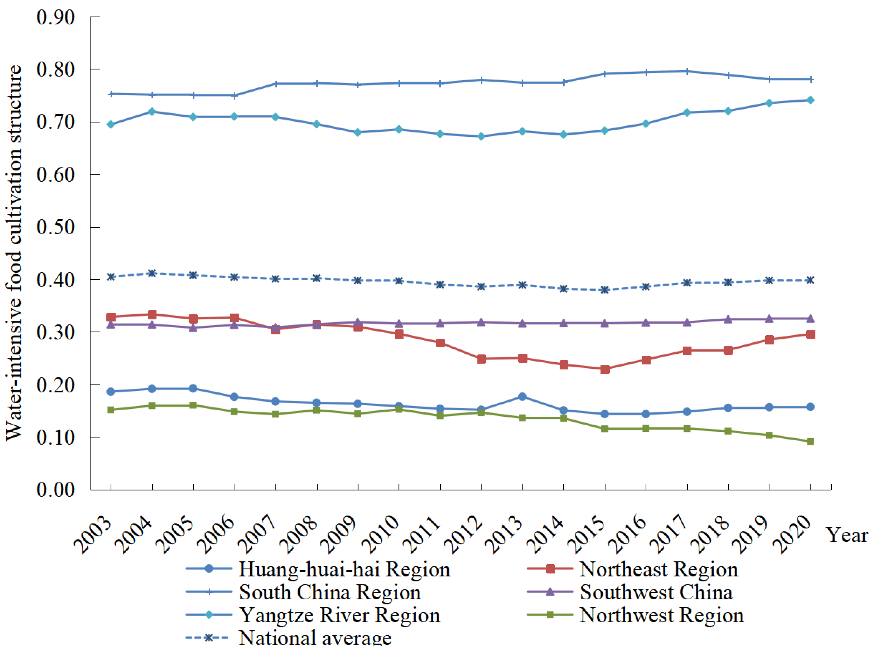
3.1. Measurement and Spatial-Temporal Variation in Water-Intensive Food Cultivation Structure

The evolution of China’s WFCS from 2003 to 2020 is shown in Figure 1. Most samples have WFCS values distributed between 0 and 1. The distribution curve of the kernel density function mainly shows two peaks with high intensity and short span, indicating that China’s WFCS is in a severe divergence trend due to changes in regional resource endowment, socio-economic development, policy, and other comprehensive factors. Over time, the nucleation density increases for the lower values of the WFCS peaks. Conversely, the nucleation density decreases for the higher values of the WFCS peaks, indicating an overall declining trend in China’s WFCS from 2003 to 2020. This was partly due to the provinces’ rapid development at the economic and social levels. At the same time, the demand for industrial and domestic water was also increasing, crowding out the water used for the production of less economically efficient food to some extent. Thus, the proportion of WFC was forced to decrease continuously. On the other hand, the growing imports of food products, led by soybeans, partially replaced domestic soybean production, thus reducing the share of WFC.

The specific WFCS in each region from 2003 to 2020 is shown in Figure 2. Affected by climate factors, socio-economic development, and water resources endowment, there were obvious differences among regions. Overall, the WFCS in South China and the middle and lower reaches of the Yangtze River showed a slightly upward trend with an obviously higher level. The climatic condition (higher precipitation) in South China and the middle and lower reaches of the Yangtze River was more suitable for the cultivation of high-water-consuming food crops such as rice and soybeans. In addition, the socio-economic development of the two regions was at a higher level in the country. The opportunity cost of water for food production was also higher. Therefore, producers preferred to grow rice and soybeans, two of the more profitable food crops. Meanwhile, the WFCS in the Southwest remained steady, while the WFCS in the Northeast showed a decreasing and then increasing trend. The WFCS in these two regions had apparently been at a medium level. The WFCS in the Huang-Huai-Hai and Northwest regions showed a decreasing trend with an obviously lower level. The climatic conditions and water endowment in the Yellow and Huaihai Sea and Northwest regions were not conducive to the production of high-water-consuming food crops such as rice and soybeans. As a result, the proportion of the high-water-consuming food crops grown was at a low level. Coupled with an increasing mismatch between food production and water distribution, the implementation of the most stringent water management system led to a continuous decline in the proportion of high-water-consuming food crops grown in the Yellow and Huaihai Sea and Northwest regions.

3.2. Empirical Analysis of the Structural Effects of Food Imports on Water-Intensive Food Cultivation

In order to facilitate the understanding of the methodology and empirical logic used in this study, a flowchart of the empirical methodology is provided in Figure 3.

3.2.1. Baseline Regression

Table 2. Baseline regression results of the effect of structural effects of food imports on water-intensive food cultivation structure.

Variables	(1)	(2)	(3)	(4)
Structural effects of food imports		−0.161 ***	−0.407 **
		(−2.929)	(−2.180)
First-order lagged term for “Structural effects of food imports”				−0.140 **
				(−2.440)
Technical environment	−3.347	−3.489	−2.737	−3.287
	(−1.353)	(−1.420)	(−1.048)	(−1.220)
Water use structure	7.474	9.965	8.519	7.245
	(0.790)	(1.058)	(0.810)	(0.749)
Irrigation ratio	11.298	12.099	16.546	8.291
	(0.597)	(0.651)	(0.715)	(0.426)
Financial support level for agriculture	−0.015	0.242	0.595	0.310
	(−0.017)	(0.273)	(0.608)	(0.331)
Disaster rate	−4.898	−5.551	−5.859	−8.547
	(−0.462)	(−0.527)	(−0.526)	(−0.759)
Agricultural machinery level	−1.392 **	−1.335 **	−1.229 **	−1.383 **
	(−2.418)	(−2.334)	(−2.018)	(−2.339)
Time fixed effects	yes	yes	yes	yes
Individual fixed effects	yes	yes	yes	yes
Phase I F-statistic values			57.83
Wald test value			4.93 **
Constant term	42.988 ***	42.388 ***	41.237 ***	42.990 ***
	(3.728)	(3.745)	(3.526)	(3.752)
Observation value	540	540	540	510

Notes: (i) *** and ** represent significant at the 1% and 5% levels, respectively. (ii) The number in parentheses are the z value.

reports the results of the model estimation of the SEFI on the WFCS (based on Equation (1)). Column (1) indicates the regression result of the control variables on the structure of food cultivation as a reference for other regression models. From the regression result in column (2), the SEFI on food cropping structure is significant at the p < 1% level with a coefficient of −0.161, indicating that each additional unit of the structural effect of food imports will reduce the WFCS by 0.161 units. This is because China’s per capita water holdings are much lower than the international average. In addition, there are differences in virtual water content among different food products. As China’s food trade deficit in soybeans and rice continues to widen, domestic food traders prefer to purchase imported soybeans and rice, which are both lower in cost and price [21]. As a result, domestic consumption of soybeans and rice has been crowded out, causing the share of the sown area to decline gradually. Similarly, the structural effects will be more pronounced in regions with higher soybean and rice imports. This reduces soybean and rice crops in the region, lowering the proportion of water-intensive food crops grown [22].

Considering the potential endogeneity of the model, the WFCS is influenced by many factors and may have the problem of missing variables, such as climatic factors, policy factors, and other influences that are unobservable. In addition, with the upgrading of WFCS, the government may encourage food trading companies to increase imports to reduce the burden of water use. Thus, there may be a reverse causality problem between the SEFI and the WFCS. To deal with the endogeneity of the model, this study relies on the instrumental variable method. “Chinese food price” and “Food imports” are closely related. “Structural effects of food imports” is calculated from “Food imports”. Thus, “Chinese food price” is theoretically correlated with the endogenous variable “Structural effects of food imports”, and is not directly related to the random error term and the WFCS in the current period. Thus, “Chinese food price” can be used as an instrumental variable in this study. First, this study tests the validity of the instrumental variable. As shown in column (3), the Wald endogeneity test is significant at the p < 1% level, indicating that the “Structural effects of food imports” is an endogenous variable. Meanwhile, the estimated F-value of 57.83 at the first stage regression is much higher than the threshold value of 10 for the weak instrumental variable test. Therefore, “Chinese food price” is suitable as an instrumental variable for the “Structural effects of food imports”. The two-stage regression result shows that the regression coefficient of the SEFI on the WFCS is significant at the p < 5% level with a coefficient of −0.407, further indicating that the SEFI can effectively mitigate the WFCS.

Considering that the negative effect of SEFI on the proportion of WFC may require a certain transmission time, the first-order lag term of the SEFI is included in the regression (based on Equation (2)). The regression result in column (4) shows that the effects of the SEFI on the WFCS are significant at the p < 5% level with a coefficient of −0.140. This suggests that each unit increase in the SEFI will result in a 0.140 unit decrease in the WFCS in the following year. Hence, it is clear that the SEFI does have a specific time lag on the regional WFCS.

3.2.2. Robustness Test

In order to further test the robustness of the baseline model results, a series of robustness tests are carried out in this study on the influence of the SEFI on the WFCS using the displacement estimation method and quantile regression. The results are shown in

Table 3. Robustness tests of the effect of structural effects of food imports on water-intensive food cultivation.

Variables	(1)	(2)	(3)	(4)
Structural effects of food imports	−0.008 ***	−0.196 ***	−0.157 ***	−0.161 **
	(−5.777)	(−2.985)	(−4.534)	(−2.418)
Technical environment	−0.408 ***	−7.707 *	−1.064	−3.489 **
	(−4.675)	(−1.956)	(−0.469)	(−2.470)
Water use structure	0.888 ***	15.133	1.488	9.965
	(4.564)	(1.585)	(0.317)	(0.682)
Irrigation ratio	0.275	2.086	7.454	12.099
	(0.694)	(0.109)	(0.212)	(1.250)
Financial support level for agriculture	0.028 *	−0.940	−2.671 **	0.242
	(1.949)	(−0.695)	(−2.016)	(0.477)
Disaster rate	−0.192	−27.298 **	−28.192 **	−5.551
	(−0.746)	(−2.393)	(−2.295)	(−0.476)
Agricultural machinery level	−0.048	−0.534	−0.291	−1.335
	(−1.066)	(−0.670)	(−0.073)	(−1.317)
Time fixed effects	no	yes	yes	yes
Individual fixed effects	no	yes	yes	yes
Constant term	3.694 ***	59.295 ***	51.801 ***	42.388 ***
	(20.038)	(3.310)	(3.676)	(5.654)
Observation value	540	510	540	540

Notes: (i) ***, ** and * represent significant at the 1%, 5%, and 10% levels, respectively. (ii) The numbers in parentheses are the z values. (iii) Models (1)–(4) are PPML, FGLS, PCSE, and bootstrap (1000 times) models, respectively.

. The result of the LR test for the effect of the SEFI on the WFCS shows that the hypothesis that the panel random disturbance terms belong to homoskedasticity is rejected. Thus, there is a heteroskedasticity problem. Moreover, the Wooldridge test result shows that the hypothesis of no within-group autocorrelation is rejected, that is, there is a within-group autocorrelation problem. Meanwhile, the food import trade in some provinces or years is zero. Therefore, the ordinary panel Tobit model may have the problem of biased estimation. To correct the estimation bias due to heteroskedasticity and within-group autocorrelation, this study uses the Poisson pseudo-maximum likelihood estimation method (PPML) [23], feasible generalized least squares (FGLS) [24], and panel-corrected standard error (PCSE) [25], respectively, for parameter estimation. The results of PPML, FGLS, and PCSE model tests are shown in columns (1)–(3) of Table 3, indicating that the impact of the SEFI on the WFCS is significantly negative, which is roughly consistent with the baseline regression results.

In addition, since the accuracy of the parameter estimation test is closely related to the setting of the parameter form, it is difficult to determine whether the parameter model setting is correct only by theoretical discussion. If there is a non-linear relationship between the SEFI and the WFCS, the regression result of the model will produce certain errors. Thus, the robustness of the baseline model is tested using non-parametric bootstrap estimation (1000 extractions) [26]. The result of the non-parametric estimation model test is shown in column (4) of Table 3. The effects of the SEFI on the WFCS are significant at the p < 1% level with a coefficient of −0.161. This shows that the SEFI does reduce the proportion of WFC in China. The regression result of the baseline model is generally robust.

3.2.3. Quantile Regression

To overcome the influence of extreme values and error terms on the estimation results and to provide a more accurate and comprehensive description of the structural effects of food imports on the structure of food cultivation at different quartiles (based on Equation (3)), this study conducts quantile regressions at 10%, 20%,…, 90% quartiles, corresponding to the results in columns (1)–(9) of

Table 4. Quantile regression results of the impact of structural effects of food imports on water-intensive food cultivation structure.

Variables	(1)	(2)	(3)	(4)	(5)	(6)	(7)	(8)	(9)
Structural effects of food imports	−0.053 **	−0.072 **	−0.120 ***	−0.127 ***	−0.145 ***	−0.155 ***	−0.269 ***	−0.283 ***	−0.277 ***
	(−2.172)	(−2.233)	(−3.139)	(−3.106)	(−3.150)	(−2.913)	(−4.873)	(−7.978)	(−6.051)
Technical environment	−5.352 ***	−8.052 ***	−7.727 ***	−9.215 ***	−12.537 ***	−17.552 ***	−22.549 ***	−23.141 ***	−13.687 ***
	(−3.831)	(−6.882)	(−3.511)	(−2.842)	(−3.106)	(−3.988)	(−5.569)	(−5.469)	(−3.367)
Water use structure	23.981 ***	33.749 ***	36.330 ***	54.838 ***	75.376 ***	65.127 ***	42.714 **	68.494 ***	75.939 ***
	(3.367)	(6.320)	(4.266)	(4.174)	(5.244)	(3.799)	(2.473)	(3.976)	(4.311)
Irrigation ratio	−9.203 ***	−10.945 **	−9.106	7.713	11.939	2.552	−39.889 **	−48.594 ***	−50.834 ***
	(−2.872)	(−1.994)	(−0.788)	(0.460)	(0.583)	(0.121)	(−2.328)	(−3.477)	(−3.823)
Financial support level for agriculture	−0.677	−0.405	0.287	0.699	0.588	−0.783	−1.974 *	−1.696	−1.076
	(−1.529)	(−0.870)	(0.625)	(1.561)	(0.823)	(−0.650)	(−1.652)	(−1.243)	(−0.863)
Disaster rate	−13.652 **	−5.594	2.804	13.215	23.047	33.058	2.610	9.570	5.642
	(−2.030)	(−0.576)	(0.290)	(0.983)	(1.251)	(1.409)	(0.142)	(0.800)	(0.611)
Agricultural machinery level	−1.666 **	−1.860 **	−1.535	−2.719 *	−3.133	−4.678 *	−2.009	0.269	−0.073
	(−2.537)	(−2.207)	(−1.350)	(−1.725)	(−1.515)	(−1.903)	(−0.781)	(0.116)	(−0.039)
Constant term	17.480 ***	18.527 **	24.798 **	18.489	11.451	37.952 *	87.406 ***	81.285 ***	78.047 ***
	(2.916)	(2.402)	(2.564)	(1.516)	(0.785)	(1.931)	(5.862)	(9.299)	(11.643)

Notes: (i) ***, ** and * represent significant at the 1%, 5%, and 10% levels, respectively. (ii) The numbers in parentheses are the z values. (iii) Models (1)–(9) represent the regression results for the 10%, 20%,…, and 90% quartiles, respectively.

, respectively. In this way, the robustness of the baseline regression is tested while analyzing the heterogeneity among different regions. The result shows that the coefficients and significance of the SEFI on the WFCS differ at different quartiles. However, the coefficients from the 10% to 90% quantile have significant and stable negative values. Once again, this validates the robustness of the baseline regression.

The coefficient of the SEFI on the WFCS slowly decreases from −0.053 to −0.277 at the 10–90% quantile. It shows that the proportion of WFC is increasingly affected by the SEFI as it increases. This is because the water endowment is still sufficient to support the production of water-intensive food crops in regions with a low proportion of WFC. However, as the proportion of WFC rises, the regional water endowment struggles to support the normal production of water-intensive food crops. At this point, the structural effect of increasing imports of water-intensive food products is stronger, thus enabling a greater reduction in the proportion of domestic water-intensive food cultivation [27].

3.2.4. Heterogeneity Analysis

To further test the regional heterogeneity of the SEFI on the WFCS, this study divided the sample into northern and southern regions based on regional characteristics (as shown in

Table 5. Heterogeneity in the impact of structural effects of food imports on water-intensive food cultivation structure in the north and south.

Region	Northern Region				Southern Region
Variables	(1)	(2)	(3)	(4)	(5)	(6)	(7)	(8)
Structural effects of food imports		−0.048 **	−0.171 *			−0.079	−12.226
		(−2.061)	(−1.685)			(−0.720)	(−0.669)
First-order lagged term for “Structural effects of food imports”				−0.046 **				−0.170
				(−2.054)				(−1.482)
Technical environment	−0.348	−0.451	−0.684	−0.205	−4.720	−5.166	−35.107	−6.928
	(−0.417)	(−0.542)	(−0.719)	(−0.247)	(−0.645)	(−0.704)	(−0.507)	(−0.808)
Water use structure	8.713 *	9.017 *	9.945 *	9.381 **	−5.915	−4.270	230.637	−5.877
	(1.835)	(1.911)	(1.862)	(2.068)	(−0.387)	(−0.277)	(0.632)	(−0.376)
Irrigation ratio	−12.045 *	−13.102 *	−15.590 *	−14.330 **	95.417 ***	99.238 ***	510.957	106.910 ***
	(−1.654)	(−1.810)	(−1.783)	(−2.021)	(2.623)	(2.694)	(0.681)	(2.780)
Financial support level for agriculture	0.139	0.372	1.000	0.442	−0.278	−0.159	7.670	0.044
	(0.336)	(0.870)	(1.471)	(1.040)	(−0.173)	(−0.099)	(0.478)	(0.026)
Disaster rate	9.707 **	9.960 **	10.878 **	6.848	−8.659	−9.819	−145.059	−10.100
	(2.319)	(2.392)	(2.321)	(1.609)	(−0.386)	(−0.438)	(−0.604)	(−0.428)
Agricultural machinery level	−3.013 ***	−2.981 ***	−3.033 ***	−2.823 ***	−0.996	−0.993	0.675	−1.051
	(−6.428)	(−6.392)	(−5.775)	(−6.078)	(−1.186)	(−1.184)	(0.107)	(−1.220)
Time fixed effects	yes	yes	yes	yes	yes	yes	yes	yes
Individual fixed effects	yes	yes	yes	yes	yes	yes	yes	yes
Phase I F-statistic values			16.31				0.45
Wald test value			3.19 *				19.66
Constant term	36.540 ***	36.686 ***	37.206 ***	34.634 ***	37.055 **	36.257 *	−59.173	34.662 *
	(5.482)	(5.651)	(7.012)	(5.498)	(1.997)	(1.950)	(−0.275)	(1.898)
Observation value	270	270	270	255	270	270	270	255

Notes: (i) ***, ** and * represent significant at the 1%, 5%, and 10% levels, respectively. (ii) The numbers in parentheses are the z values.

). The regression result for the northern region sample is shown in columns (1)–(4), where column (1) shows the regression result of the control variables on the WFCS. As seen in columns (2)–(4), the regression results of either the baseline regression model, the inclusion of the instrumental variable, or the first-order lag term of the SEFI show that the SEFI has a significant negative effect on the WFCS in the northern region, similar to the result of the full-sample regression. The regression result for the southern region sample is shown in columns (5)–(8), where column (5) regresses the control variables on the WFCS. As seen in columns (6)–(8), the regression result for either the baseline regression model, the inclusion of instrumental variables, or the inclusion of the first-order lag term for the SEFI shows that the SEFI on the WFCS is not significant, unlike the result of the full-sample regression.

The SEFI is more negative on the proportion of WFC in the north than in the south. This is because of the lower endowment of water resources in the north, combined with the mismatch between the distribution of arable land and water resources and climatic factors, etc. Without some consumer demand for high-water-consuming food products such as soybeans and rice, farmers prefer to spontaneously grow low-water-consuming food crops, such as wheat and corn [28]. In this case, food imports are able to compensate for the consumption demand of high-water-consuming agricultural products in the northern region, making the proportion of low-water-consuming food crops in the northern region grow rapidly, and thus causing the proportion of WFC to gradually decrease. Conversely, southern regions with higher water endowments, influenced by climatic conditions and production profitability factors, are more inclined to spontaneously grow high-water-consuming food crops such as soybeans and rice, while reducing the proportion of less profitable food crops such as wheat and corn. Thus, the SEFI has a less negative impact on the WFCS in the south than in the north [29].

In addition, there may be significant differences in food production characteristics between major and non-major food production areas. In this study, samples are divided into major and non-major food-producing areas for testing based on the characteristics of the producing areas (as shown in

Table 6. Heterogeneity in the effect of structural effects of food imports on water-intensive food cultivation structure in different production areas.

Region	Major Food-Producing Areas				Non-Major Food-Producing Areas
Variables	(1)	(2)	(3)	(4)	(5)	(6)	(7)	(8)
Structural effects of food imports		−0.081 ***	−0.072 **			−0.197	−1.404
		(−4.143)	(−1.990)			(−1.545)	(−1.471)
First-order lagged term for “Structural effects of food imports”				−0.068 ***				−0.185
				(−3.669)				(−1.391)
Technical environment	−1.679	−1.481	−1.539	−0.891	−3.696	−3.631	−2.174	−3.853
	(−1.103)	(−1.005)	(−0.982)	(−0.640)	(−1.008)	(−0.995)	(−0.498)	(−0.945)
Water use structure	50.945 ***	57.771 ***	57.816 ***	71.378 ***	4.977	7.241	16.194	3.943
	(3.181)	(3.715)	(3.387)	(4.732)	(0.391)	(0.567)	(0.825)	(0.300)
Irrigation ratio	−14.443	−14.467	−12.102	−25.120 *	19.830	21.325	29.765	19.629
	(−0.917)	(−0.951)	(−0.742)	(−1.701)	(0.787)	(0.843)	(0.798)	(0.746)
Financial support level for agriculture	1.669 ***	1.700 ***	1.725 ***	1.616 ***	0.370	0.656	2.093	0.773
	(4.196)	(4.419)	(4.223)	(4.417)	(0.208)	(0.367)	(0.841)	(0.408)
Disaster rate	13.687 **	14.373 ***	14.006 **	11.158 **	−22.480	−23.595	−29.107	−24.030
	(2.516)	(2.730)	(2.505)	(2.210)	(−1.283)	(−1.352)	(−1.371)	(−1.301)
Agricultural machinery level	−2.255 ***	−2.195 ***	−2.173 ***	−1.674 ***	−1.145	−1.102	−0.879	−1.214
	(−3.619)	(−3.641)	(−3.392)	(−2.922)	(−1.458)	(−1.408)	(−0.932)	(−1.499)
Time fixed effects	yes	yes	yes	yes	yes	yes	yes	yes
Individual fixed effects	yes	yes	yes	yes	yes	yes	yes	yes
Phase I F-statistic values			97.90				7.43
Wald test value			3.78 *				2.72
Constant term	37.585 ***	34.200 ***	33.479 ***	30.309 ***	40.064 **	40.932 **	47.317 **	42.708 **
	(3.186)	(3.044)	(3.414)	(2.785)	(2.437)	(2.477)	(2.239)	(2.522)
Observation value	234	234	234	221	306	306	306	289

Notes: (i) ***, ** and * represent significant at the 1%, 5%, and 10% levels, respectively. (ii) The numbers in parentheses are the z values.

). The regression results for the sample of major food-producing areas are shown in columns (1)–(4), where column (1) shows the regression result of control variables on food cultivation structure. As can be seen from columns (2)–(4), the regression results for both the baseline regression model and the inclusion of instrumental variables or the inclusion of the first-order lag term for the SEFI show that the SEFI has a significant negative effect on the WFCS, which is similar to the full-sample regression result except for the change in the coefficients. The regression results for the sample of non-major food-producing areas are shown in columns (5)–(8), where column (5) shows the regression result of control variables on the WFCS. As seen in columns (6)–(8), the regression result for the baseline regression model, the inclusion of instrumental variables, and the inclusion of the first-order lag term for the SEFI show that the effects of the SEFI on the WFCS are not significant and differ significantly from the full sample regression result.

Meanwhile, the SEFI has a more substantial negative effect on the proportion of WFC in major food-producing areas than in non-major ones. This is because the proportion of water used for food production to total usage of water in the major food-producing areas has been high for a long time. Imports of unit water-intensive food products exert more substantial structural effects on the major production areas. In addition, the scale effect of the major production areas makes food production more water-efficient. The domestic water resources saved by the SEFI can be used to produce more low-water-consumption food crops such as wheat and corn [30]. Conversely, the share of water used for food production in total water use in non-major food-producing areas has been low for a long time, and imports of water-intensive food products per unit have weaker structural effects on non-major food-producing areas. At the same time, food production in non-major food-producing areas is less water-efficient. The domestic water resources saved by the SEFI can produce fewer low-water-use food crops. Therefore, the SEFI has a less negative impact on the proportion of WFC in non-major food-producing areas than in major ones [31].

3.2.5. Spatial Spillover Effect

First, this study measures the global Moran’s I index of the WFCS in 30 provincial-level administrative regions of China from 2003 to 2020 using the “proximity weight matrix”. The measurement results are shown in

Table 7. Spatially autocorrelated Moran’s I index of water-intensive food cultivation structure.

Year	Proximity Weight Matrix	Year	Proximity Weight Matrix	Year	Proximity Weight Matrix
2003	0.569 ***	2009	0.640 ***	2015	0.660 ***
2004	0.641 ***	2010	0.635 ***	2016	0.653 ***
2005	0.589 ***	2011	0.692 ***	2017	0.637 ***
2006	0.628 ***	2012	0.642 ***	2018	0.677 ***
2007	0.625 ***	2013	0.651 ***	2019	0.631 ***
2008	0.654 ***	2014	0.101 ***	2020	0.646 ***

Notes: (i) *** represent significant at the 1% levels, respectively.

(based on Equation (4)). The spatial autocorrelation coefficients are positive and pass the significance test for all years, indicating that the WFCS of the 30 provincial administrative regions in China selected for the sample does have spatial autocorrelation. It also indicates a strong positive global spatial correlation and a significant spatial clustering phenomenon in China’s WFCS from 30 provincial-level administrative regions from 2003 to 2020. That is, provinces with high WFCS are clustered, and provinces with low WFCS are adjacent. Therefore, spatial econometric models should be further introduced for analysis. Moreover, the spatial effects should be considered as a means to compensate for measurement bias in models that do not consider geographical spatial distribution factors.

From column (1) in

Table 8. A spatial Dubin model of the effect of structural effects of food imports on water-intensive food cultivation structure.

Variables	(1)	(2)
Structural effects of food imports	0.423 ***
	(9.936)
First-order lagged term for “Structural effects of food imports”	−0.137 ***	−0.263 **
	(−3.368)	(−2.334)
Technical environment	−3.923	−12.509 ***
	(−1.614)	(−2.804)
Water use structure	0.018	45.744 ***
	(0.002)	(2.714)
Irrigation ratio	18.850	0.852
	(1.396)	(0.039)
Financial support level for agriculture	−0.740	−2.011
	(−0.975)	(−1.365)
Disaster rate	−1.542	−27.869
	(−0.128)	(−1.481)
Agricultural machinery level	−0.047	−0.703
	(−0.080)	(−0.770)
Time fixed effects	yes	yes
Individual fixed effects	yes	yes
Observation value	510	510

Notes: (i) *** and ** represent significant at the 1% and 5% levels, respectively. (ii) The numbers in parentheses are the z values.

(based on Equations (5) and (6)), the coefficient of the spatial lag term of the WFCS on the current WFCS in the dynamic spatial panel Durbin model measured by the inverse distance weights is significant at the 1% level and has a coefficient of 0.423, indicating a positive correlation effect of the WFCS among regions. Again, it proves that the WFCS has some spatial dependence. It can also be seen that the coefficient of the SEFI on the WFCS is significant at the 1% level and has a coefficient of −0.137. Based on the estimation result in column (2), it is also found that the effect of the SEFI from other regions on the regional WFCS has a coefficient of −0.263 and passes the significance test at the 1% level. From this view, the extent to which the SEFI negatively affects the WFCS is underestimated in the model that does not consider spatial effects.

Since the dynamic spatial panel Durbin model (PSDM) is not a linear regression, the estimated coefficients do not directly capture the marginal effect of the SEFI on the WFCS. Therefore, the estimated coefficients need to be further decomposed into direct, indirect, and total effects with the help of partial differential methods. Meanwhile, PSDM also classifies the three effects into long-term and short-term types (as shown in

Table 9. Decomposition results of spatial spillover effect of structural effects of food imports on water-intensive food cultivation structure.

Variables	(1)	(2)	(3)	(4)	(5)	(6)
Structural effects of food imports	−0.147 ***	−0.296 **	−0.443 ***	−0.270 ***	−0.609 **	−0.878 ***
	(−3.743)	(−2.425)	(−3.392)	(−3.838)	(−2.420)	(−3.183)
Technical environment	−4.088 *	−13.997 ***	−18.085 ***	−7.729 *	−28.019 ***	−35.749 ***
	(−1.750)	(−3.002)	(−3.285)	(−1.871)	(−2.978)	(−3.187)
Water use structure	1.262	49.144 ***	50.405 ***	4.244	95.084 ***	99.328 ***
	(0.155)	(2.826)	(3.077)	(0.303)	(2.911)	(3.104)
Irrigation ratio	19.216	3.738	22.953	33.737	11.837	45.574
	(1.505)	(0.157)	(1.021)	(1.538)	(0.257)	(0.999)
Financial support level for agriculture	−0.760	−2.341	−3.101	−1.431	−4.738	−6.169
	(−0.988)	(−1.451)	(−1.538)	(−1.044)	(−1.442)	(−1.511)
Disaster rate	−2.552	−29.875	−32.426	−5.797	−58.864	−64.661
	(−0.208)	(−1.410)	(−1.394)	(−0.271)	(−1.388)	(−1.356)
Agricultural machinery level	−0.086	−0.856	−0.942	−0.186	−1.675	−1.861
	(−0.157)	(−0.847)	(−0.805)	(−0.194)	(−0.841)	(−0.795)

Notes: (i) ***, ** and * represent significant at the 1%, 5%, and 10% levels, respectively. (ii) The numbers in parentheses are the z values. (iii) Model (1)–(6) represent the short-run direct effect, short-run indirect effect, short-run total effect, long-run direct effect, long-run indirect effect, and long-run total effect in the spatial econometric regression results, respectively.

).

From the direct effect decomposition results, column (1) shows that the short-term direct effect of the SEFI on the WFCS is significant at the 1% level and has a coefficient of −0.147. It indicates that for every 1-unit increase in the SEFI in the region after considering the feedback effect (i.e., including the structural effects of food imports in the area, which affects the regional WFCS through the one in neighboring regions), the proportion of WFC in the area will decrease by 0.147 units. Column (4) shows that the short-term direct effect of the SEFI on the WFCS is significant at the 1% level with a coefficient of −0.270, indicating that for every 1-unit increase in the SEFI in the region after considering the feedback effect, the WFC facilitation in the region will decrease by 0.270 units. This shows that the long-term direct effect of the SEFI on the WFCS is higher than the short-term direct effect.

From the decomposition results of the indirect effect, column (2) shows that the short-term indirect effect of the SEFI on the WFCS is significant at the 5% level with a coefficient of −0.296, indicating that for every 1-unit increase in the SEFI in this region, the WFCS in neighboring regions will decrease by 0.296 units. Column (5) shows the long-term indirect effect of the SEFI on the WFCS is significant at the 5% level with a coefficient of −0.609, indicating that for every 1-unit increase in the SEFI in the region, the WFCS in neighboring regions will decrease by 0.609 units. This shows that the long-term indirect effect of the SEFI on the WFCS in neighboring areas is higher than the short-term indirect effect. From the decomposition results of the total effect, column (3) shows that the total short-term effect of the SEFI on the WFCS passes the significance test at the 1% level with a coefficient of −0.443, which means that every 1-unit increase in the SEFI in the region reduces the WFCS within the region and adjacent regions by 0.443 units. Column (6) shows that the total long-term effect of the structural effects of food imports on the WFCS passes the significance test at the 1% level with a coefficient of 0.878. That is, each 1-unit increase in the SEFI in the region reduces the WFCS within the region and adjacent regions by 0.878 units. It can be seen that the total long-term effect of the SEFI on the WFCS is higher than the total short-term effect.

The results above suggest that the increase in the SEFI in the region can reduce the proportion of WFC in the region and neighboring regions.

3.2.6. Discussion

While quantifying as accurately as possible the total welfare gained from trade, established scholars are further exploring all possible sources of trade welfare, including the self-selection effect of exports, the growth effect of the type of imports, and the trade-for-competition effect. At the same time, scholars also focus on the impact of import trade on industrial development and economic growth. In the study of the welfare effects of food import trade, they mainly focus on the regulation of food imports on domestic supply and demand and the promotion of agricultural economic growth. However, studies exploring the virtual water flows induced by the food import trade, which ultimately lead to changes in the food cultivation structure of importing countries, are fewer and more at the stage of descriptive analysis. Using the Tobit model, quantile regression, sub-sample regression, and spatial measurement, this study utilizes China’s provincial panel data from 2003 to 2020, confirming that the food import structure will improve the domestic food cultivation structure. The reasons for the results are as follows:

By importing relatively scarce domestic factor resources and exporting relatively abundant factor resources, we can effectively reduce domestic production costs and thus maximize benefits. Since the production of different food products requires different proportions of factor resource inputs, the factor endowments theory is shown in the process of food production and regional trade as follows: a country or region should transfer out food products with factor endowments and transfer in food products with scarce factor resources, so as to reduce the consumption of scarce factor resources and save food production costs. China’s per capita water resource possession is 25% of the world average, which is far lower than the international average, so the water resource elements are all scarce elements in China. According to the factor endowments theory, due to the heterogeneity of factor prices at home and abroad, which leads to differences in food production costs, Chinese food enterprises have been driven by profit maximization to spontaneously apply to import water-intensive food products, forming SEFI to compensate for scarce factors. Imported food products have lower cost and price than domestic ones. Thus, rational food traders will buy lower-priced imported products to replace corresponding higher-priced domestic ones, which will then experience a decline in their demand. This will be transmitted to the food production side through the invisible hand of the market, reducing the output of corresponding domestic food products. Moreover, this action indirectly restructures China’s domestic food production, reduces the production of water-intensive food products, and effectively alleviates the pressure of water scarcity in the food production process.

4. Conclusions

Based on the factor endowments theory, this study further explores the impact of SEFI on China’s food cultivation structure from the perspective of product structure. First, the WFCS is measured, and results are elaborated and analyzed. Second, an empirical model of the effect of SEFI on the food cultivation structure in China is constructed. Third, the effects of the SEFI on the WFCS are empirically tested separately, and robustness tests, heterogeneity analysis, and spatial spillover effect tests are conducted. In this way, we undertake in-depth analysis of the mechanism of the structural effects of food imports on the food cultivation structure in China. The results show that: (i) The WFCS in South China and the middle and lower reaches of the Yangtze River shows a slightly increasing trend with an obviously higher level. The WFCS in the Huang-Huai-Hai and Northwest regions shows a decreasing trend with an obviously lower level. (ii) The SEFI does effectively reduce the WFCS. On average, each additional 100,000 tons of food imports would result in a 0.161% decrease in the share of WFC. (iii) Using the Poisson pseudo-maximum likelihood estimation method (PPML), feasible generalized least squares (FGLS), panel-corrected standard error (PCSE), and non-parametric estimation, robustness tests show that the baseline model regression result is more robust. Among them, the quantile regression result finds that the negative effect of the SEFI on the WFCS grows with the development of the WFCS. (iv) The sub-sample regression finds that the SEFI has a stronger negative effect on the proportion of WFC in the north than in the south. Moreover, the SEFI has a stronger negative effect on the proportion of WFC in major food-producing regions than in non-major food-producing regions. (v) From the results of the spatial econometric model, there is a positive association between the WFCS in neighboring regions. An increase in the SEFI in the region can reduce the proportion of WFC in the region and neighboring regions.

The above conclusions provide some new ideas for adjusting the structure of food imports, optimizing the structure of food cultivation, and saving water resources. The premise of rational adjustment of the food import structure is to accurately measure the water demand of broad food production, strictly classify the water and land consumption of food products, and implement import strategies differently from the perspective of water conservation. With the rapid improvement in the socio-economy, the dietary structure of Chinese residents is also being upgraded, and the demand for feed grains such as soybeans and corn is increasing significantly. In addition, the SEFI has a strong negative effect on the proportion of WFC in northern regions and major food-producing regions. Thus, within the limits of China’s food import quota, the government should encourage an appropriate increase in imports of food products with high virtual water content in these regions, such as soybeans and rice, and reduce the import of soybeans and rice in the southern region and non-major food-producing regions. Under the goal of satisfying Chinese residents’ demand for diversified food products, and taking into account the sustainable use of domestic water and arable land resources, more food products with high water and land consumption, such as meat, eggs, milk, and aquatic products, should be imported, compared to food products such as soybeans, rice, wheat and corn, so that China’s food dependence on foreign countries is guaranteed to be within a relatively safe range.

References

1. Du, T.S.; Kang, S.Z.; Zhang, X.Y.; Zhang, J.H. China’s food security is threatened by the unsustainable use of water resources in North and Northwest China. Food Energy Secur. 2014, 3, 7–18. [Google Scholar] [CrossRef]
2. Sun, S.K.; Lu, Y.J.; Gao, H.; Jiang, T.T.; Du, X.Y.; Shen, T.X.; Wu, P.T.; Wang, Y.B. Impacts of food wastage on water resources and environment in China. J. Clean. Prod. 2018, 185, 732–739. [Google Scholar] [CrossRef]
3. Han, X.X.Q.; Zhao, Y.; Gao, X.R.; Jiang, S.; Lin, L.X.; An, T.L. Virtual water output intensifies the water scarcity in Northwest China: Current situation, problem analysis and countermeasures. Sci. Total Environ. 2021, 765, 144276. [Google Scholar] [CrossRef] [PubMed]
4. Olayungbo, D.O. Global oil price and food prices in food importing and oil exporting developing countries: A panel ARDL analysis. Heliyon 2021, 7, e06357. [Google Scholar] [CrossRef] [PubMed]
5. Cai, B.M.; Hubacek, K.; Feng, K.S.; Zhang, W.; Wang, F.; Liu, Y. Tension of Agricultural Land and Water Use in China’s Trade: Tele-Connections, Hidden Drivers and Potential Solutions. Environ. Sci. Technol. 2020, 54, 5365–5375. [Google Scholar] [CrossRef] [PubMed] [Green Version]
6. Chapagain, A.K.; Hoekstra, A.Y.; Savenije, H.H.G. Water saving through international trade of agricultural products. Hydrol. Earth Syst. Sci. 2006, 10, 455–468. [Google Scholar] [CrossRef] [Green Version]
7. Chartres, C.J.; Noble, A. Sustainable intensification: Overcoming land and water constraints on food production. Food Secur. 2015, 7, 235–245. [Google Scholar] [CrossRef]
8. Grzelak, A.; Guth, M.; Matuszczak, A.; Czyzewski, B.; Brelik, A. Approaching the environmental sustainable value in agriculture: How factor endowments foster the eco-efficiency. J. Clean. Prod. 2019, 241. [Google Scholar] [CrossRef]
9. Redding, S.J. Goods trade, factor mobility and welfare. J. Int. Econ. 2016, 101, 148–167. [Google Scholar] [CrossRef] [Green Version]
10. Condon, A.G. Drying times: Plant traits to improve crop water use efficiency and yield. J. Exp. Bot. 2020, 71, 2239–2252. [Google Scholar] [CrossRef]
11. Chen, M.L.; Jin, J.L.; Ning, S.W.; Zhou, Y.L.; Udmale, P. Early Warning Method for Regional Water Resources Carrying Capacity Based on the Logical Curve and Aggregate Warning Index. Int. J. Environ. Res. Public. Health 2020, 17, 2206. [Google Scholar] [CrossRef] [PubMed] [Green Version]
12. Alessa, L.; Kliskey, A.; Lammers, R.; Arp, C.; White, D.; Hinzman, L.; Busey, R. The arctic water resource vulnerability index: An integrated assessment tool for community resilience and vulnerability with respect to freshwater. Environ. Manag. 2008, 42, 523–541. [Google Scholar] [CrossRef] [PubMed]
13. Sun, J.; Mooney, H.; Wu, W.B.; Tang, H.J.; Tong, Y.X.; Xu, Z.C.; Huang, B.R.; Cheng, Y.Q.; Yang, X.J.; Wei, D.; et al. Importing food damages domestic environment: Evidence from global soybean trade. Proc. Natl. Acad. Sci. USA 2018, 115, 5415–5419. [Google Scholar] [CrossRef] [Green Version]
14. Chen, Z.M.; Chen, G.Q. Virtual water accounting for the globalized world economy: National water footprint and international virtual water trade. Ecol. Indic. 2013, 28, 142–149. [Google Scholar] [CrossRef]
15. Dalin, C.; Hanasaki, N.; Qiu, H.G.; Mauzerall, D.L.; Rodriguez-Iturbe, I. Water resources transfers through Chinese interprovincial and foreign food trade. Proc. Natl. Acad. Sci. USA 2014, 111, 9774–9779. [Google Scholar] [CrossRef]
16. Ali, T.; Huang, J.K.; Wang, J.X.; Xie, W. Global footprints of water and land resources through China’s food trade. Glob. Food Secur.-Agric. Policy Econ. Environ. 2017, 12, 139–145. [Google Scholar] [CrossRef]
17. Buchthal, O.; Nelson-Hurwitz, D.; Hsu, L.; Byers, M.; Banna, J. Identifying Urban Immigrant Food-Cultivation Practices for Culturally-Tailored Garden-Based Nutrition Programs. J. Immigr. Minor. Health 2020, 22, 778–785. [Google Scholar] [CrossRef]
18. Moran, P.A. A test for the serial independence of residuals. Biometrika 1950, 37, 178–181. [Google Scholar] [CrossRef]
19. Dubin, R. Spatial lags and spatial errors revisited: Some Monte Carlo evidence. In Spatial and Spatiotemporal Econometrics; LeSage, J.P., Pace, R.K., Eds.; Advances in Econometrics: New York, NY, USA, 2004; Volume 18, pp. 75–98. [Google Scholar]
20. Zhao, D.D.; Hubacek, K.; Feng, K.S.; Sun, L.X.; Liu, J.G. Explaining virtual water trade: A spatial-temporal analysis of the comparative advantage of land, labor and water in China. Water Res. 2019, 153, 304–314. [Google Scholar] [CrossRef]
21. De Loecker, J.; Goldberg, P.K.; Khandelwal, A.K.; Pavcnik, N. Prices, Markups, and Trade Reform. Econometrica 2016, 84, 445–510. [Google Scholar] [CrossRef] [Green Version]
22. Shao, L.; Guan, D.B.; Wu, Z.; Wang, P.S.; Chen, G.Q. Multi-scale input-output analysis of consumption-based water resources: Method and application. J. Clean. Prod. 2017, 164, 338–346. [Google Scholar] [CrossRef] [Green Version]
23. Hoang, N.T.T.; Truong, H.Q.; Dong, C.V. Determinants of Trade between Taiwan and ASEAN Countries: A PPML Estimator Approach. Sage Open 2020, 10. [Google Scholar] [CrossRef]
24. Rocha, A.; Miranda, M.C. A Robust Version of the FGLS Estimator for Panel Data. In Proceedings of the 25th Congress of the Portuguese-Statistical-Society (SPE), University of Évora, Electr Network, Évora, Portugal, 13–16 October 2021; pp. 325–335. [Google Scholar]
25. Dabrowski, P.S. Novel PCSE-based approach of inclined structures geometry analysis on the example of the Leaning Tower of Pisa. Measurement 2022, 189, 110462. [Google Scholar] [CrossRef]
26. Liu, W.C.; Lai, S.M.; Chen, H.W. A topological similarity-based bootstrapping method for inferring food web parameters. Ecol. Res. 2017, 32, 797–809. [Google Scholar] [CrossRef]
27. Lu, Y.J.; Yan, D.H.; Qin, T.L.; Song, Y.F.; Weng, B.S.; Yuan, Y.; Dong, G.Q. Assessment of Drought Evolution Characteristics and Drought Coping Ability of Water Conservancy Projects in Huang-Huai-Hai River Basin, China. Water 2016, 8, 378. [Google Scholar] [CrossRef]
28. Niu, S.D.; Lyu, X.; Gu, G.Z. A New Framework of Green Transition of Cultivated Land-Use for the Coordination among the Water-Land-Food-Carbon Nexus in China. Land 2022, 11, 933. [Google Scholar] [CrossRef]
29. Qi, Y.Y.; Farnoosh, A.; Lin, L.; Liu, H. Coupling coordination analysis of China’s provincial water-energy-food nexus. Environ. Sci. Pollut. Res. 2022, 29, 23303–23313. [Google Scholar] [CrossRef] [PubMed]
30. Cheng, R.; Mantovani, A.; Frazzoli, C. Analysis of Food Safety and Security Challenges in Emerging African Food Producing Areas through a One Health Lens: The Dairy Chains in Mali. J. Food Prot. 2017, 80, 57–67. [Google Scholar] [CrossRef] [PubMed]
31. Zhang, Y.J.; Yuan, S.C.; Wang, J.; Cheng, J.; Zhu, D.L. How Do the Different Types of Land Costs Affect Agricultural Crop-Planting Selections in China? Land 2022, 11, 1890. [Google Scholar] [CrossRef]
Figure 1. Estimated kernel density index of high water-intensive food cultivation structure, 2003–2020.
Water 15 02800 g001
Figure 2. Water-intensive food cultivation structure by region, 2003–2020.
Water 15 02800 g002
Figure 3. Flowchart of the empirical methodology.
Water 15 02800 g003