


Numerical–Experimental Study of Scour in the Discharge of a Channel: Case of the Carrizal River Hydraulic Control Structure, Tabasco, Mexico


Abstract
:1. Introduction
2. Methods
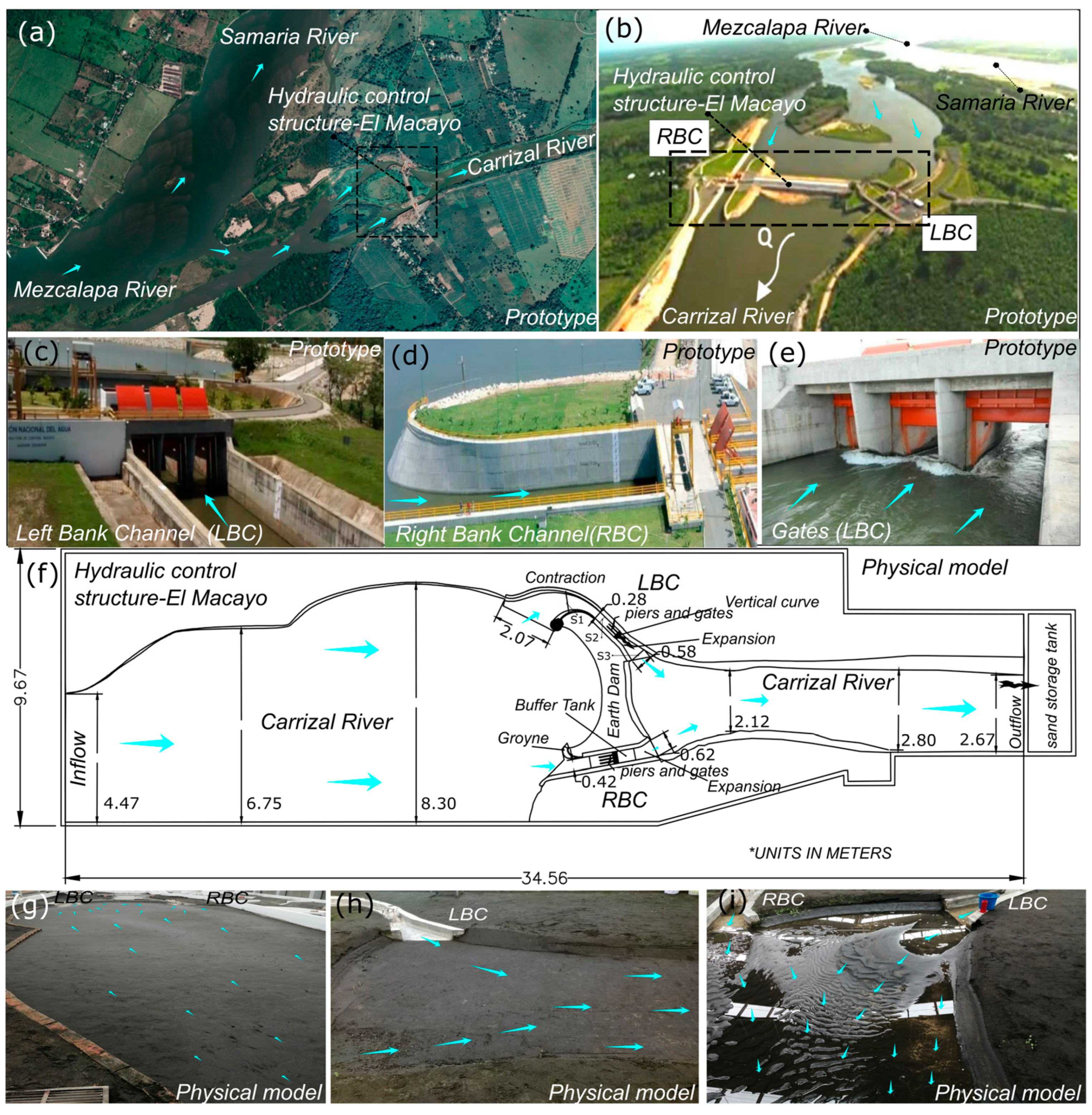
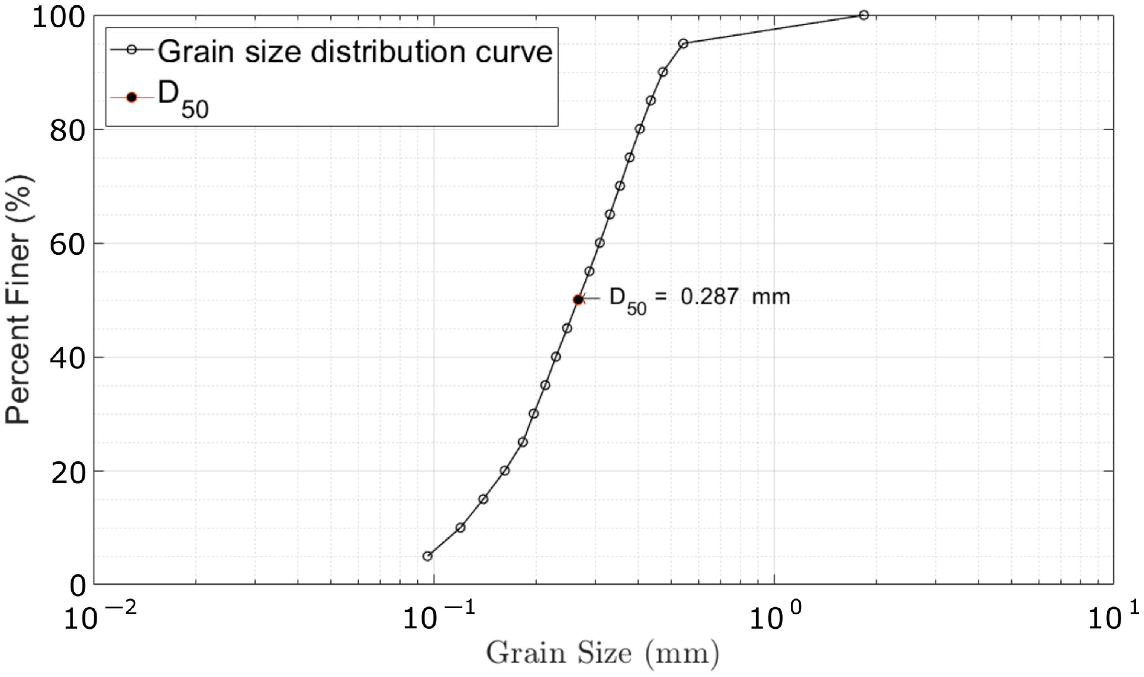
2.1. Physical Model
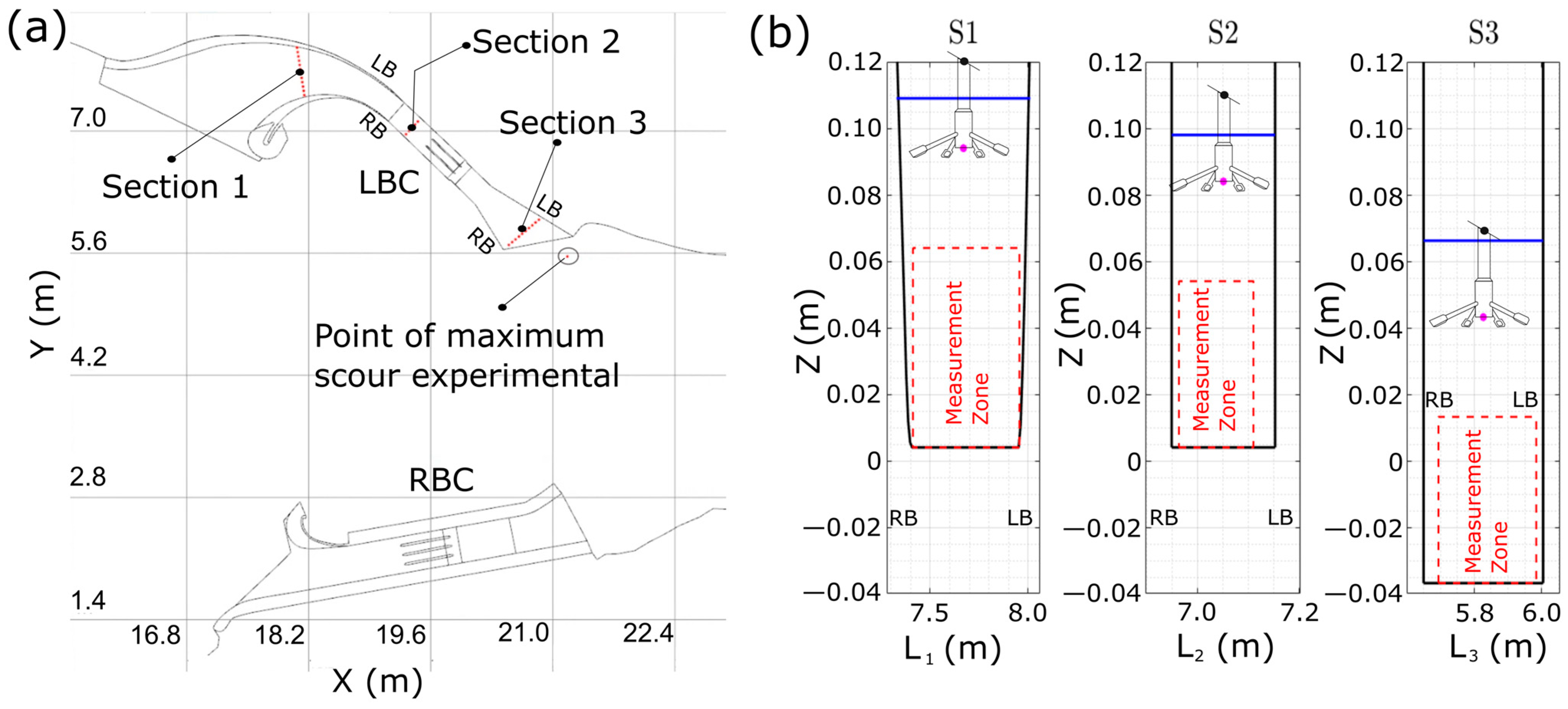
Flow Field Measurements
2.2. Numerical Model
3. Results
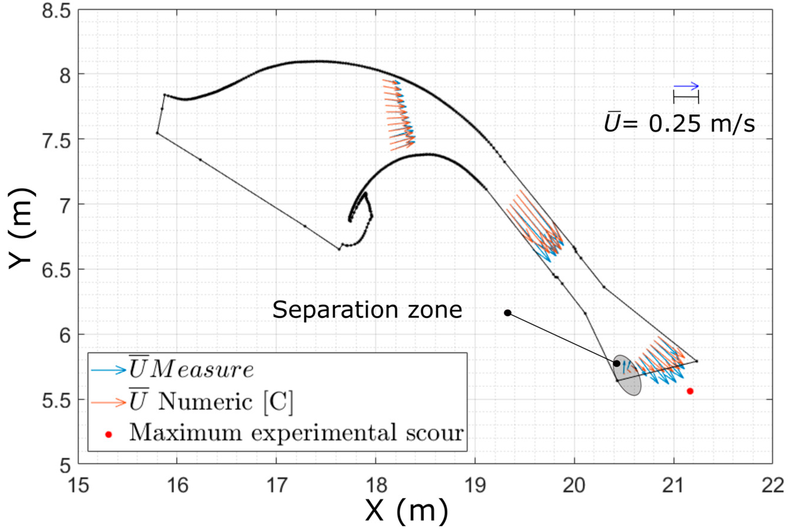
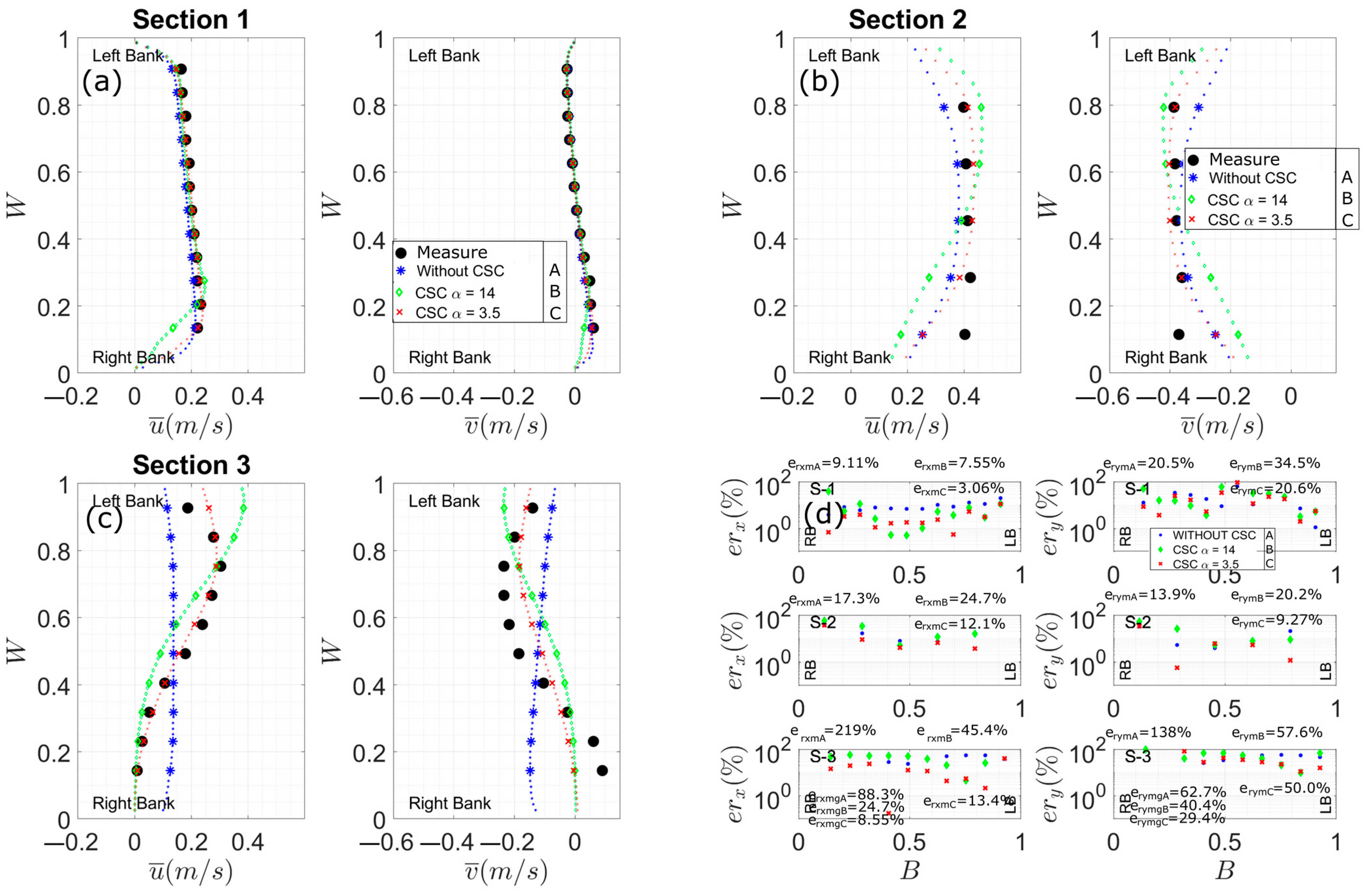
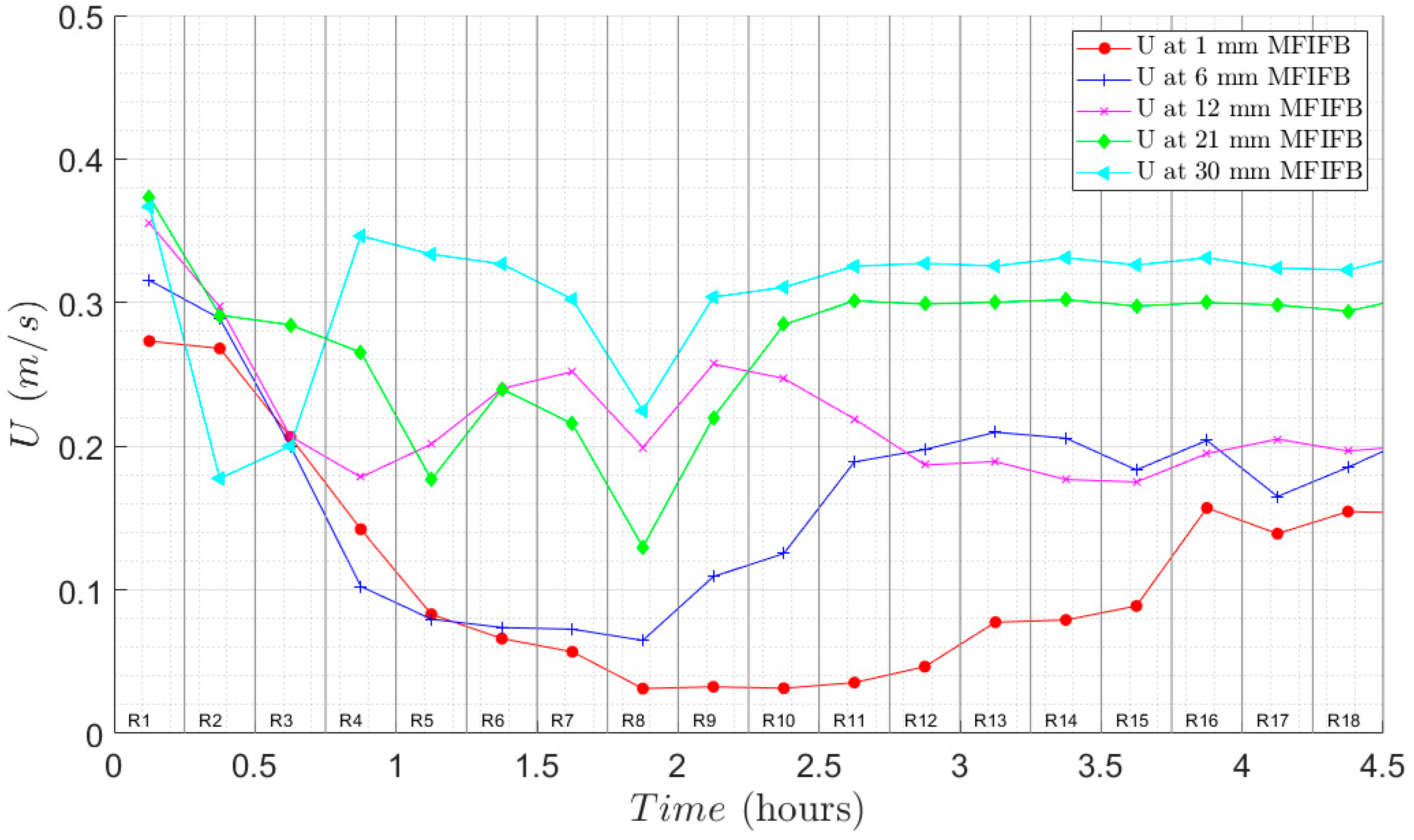
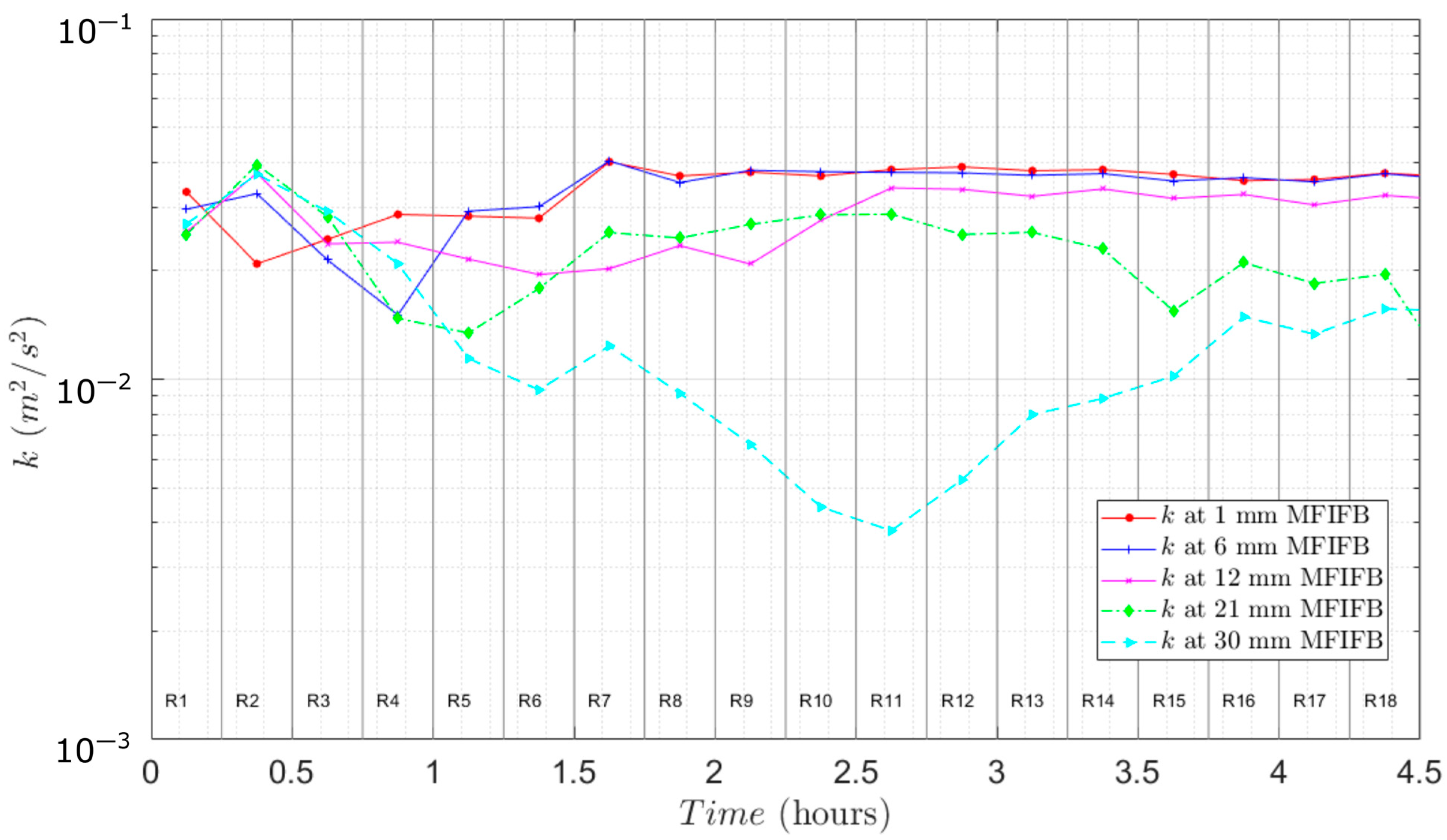
3.1. Velocity Field Measurement
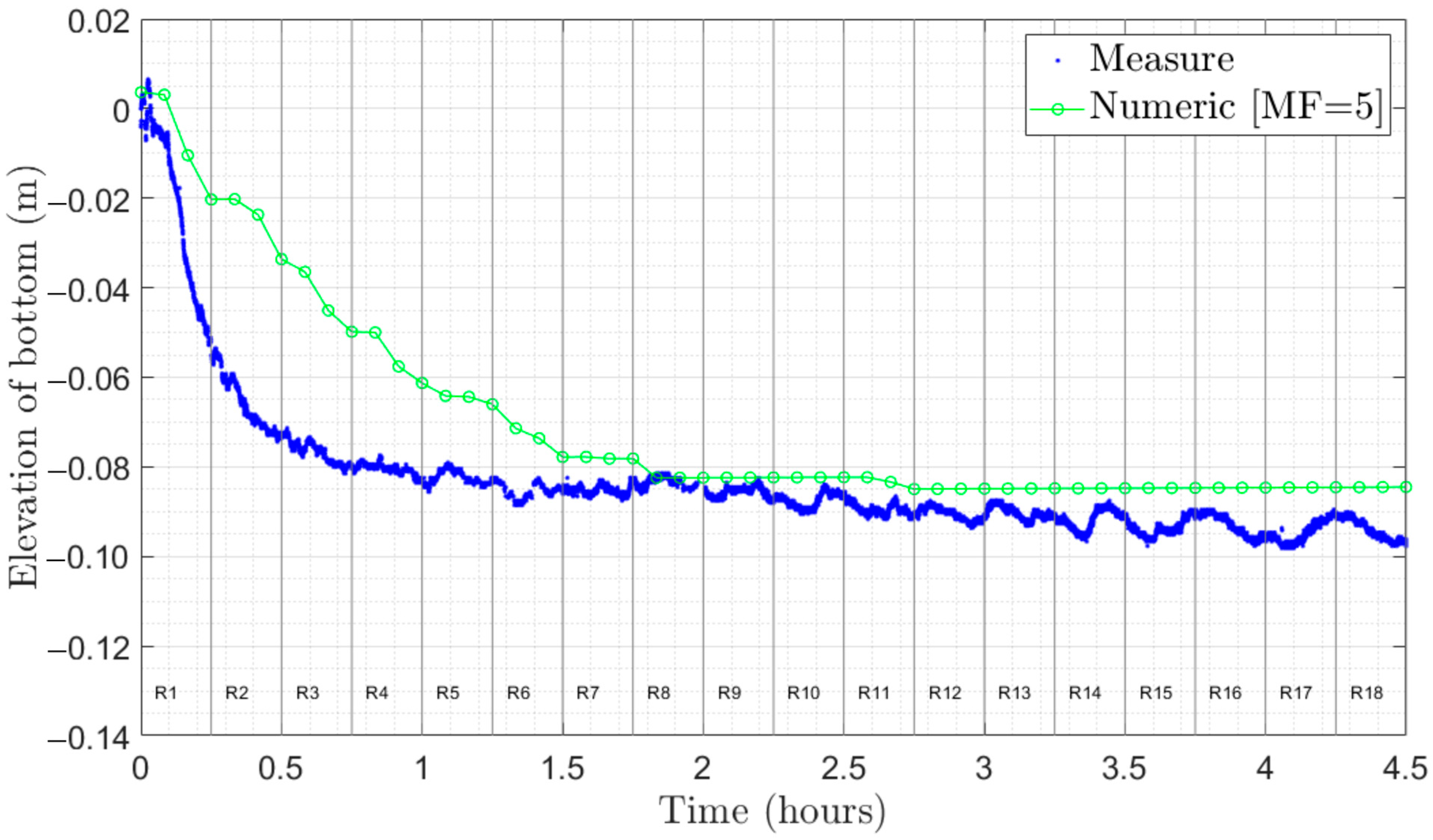
3.2. Numerical Model Calibration
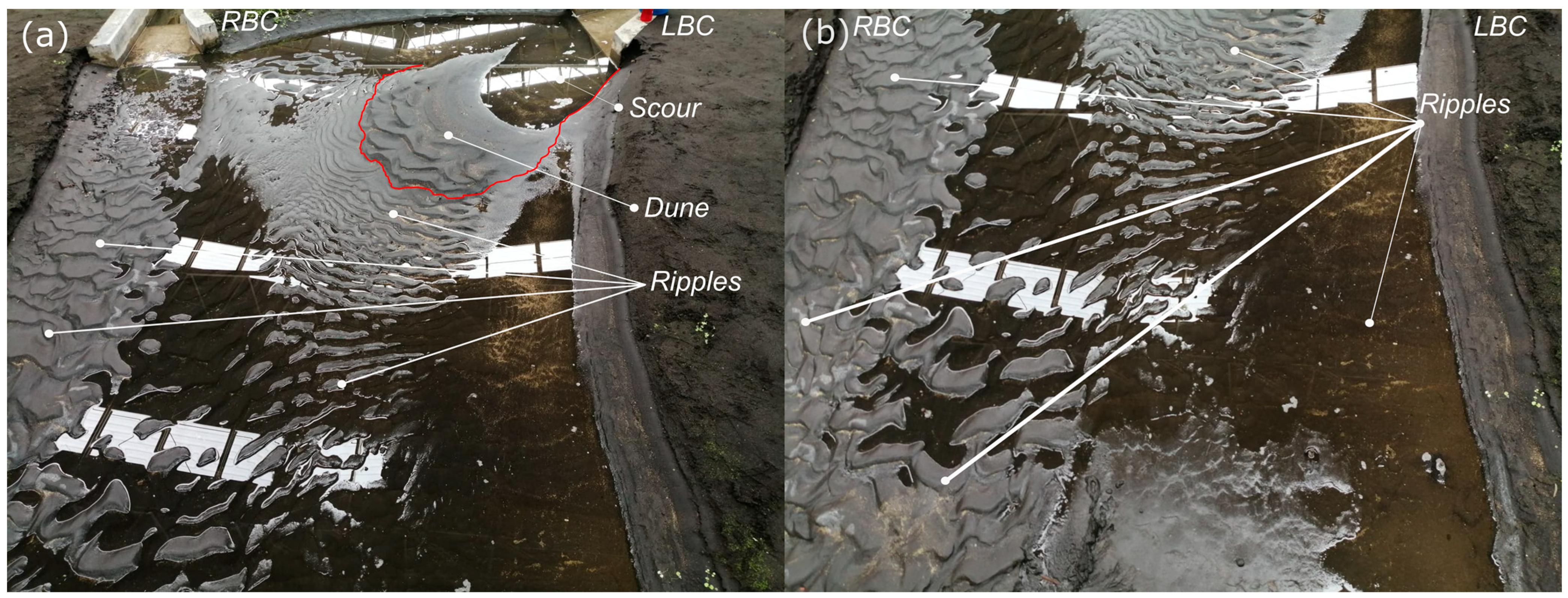
3.3. Scour
4. Discussion
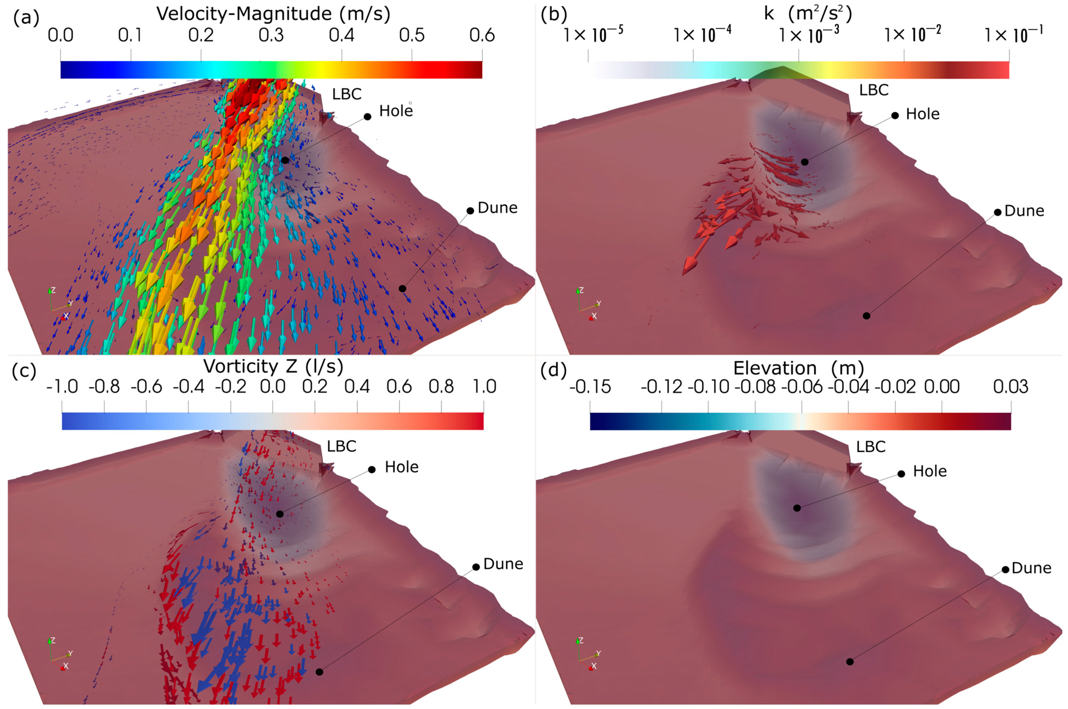
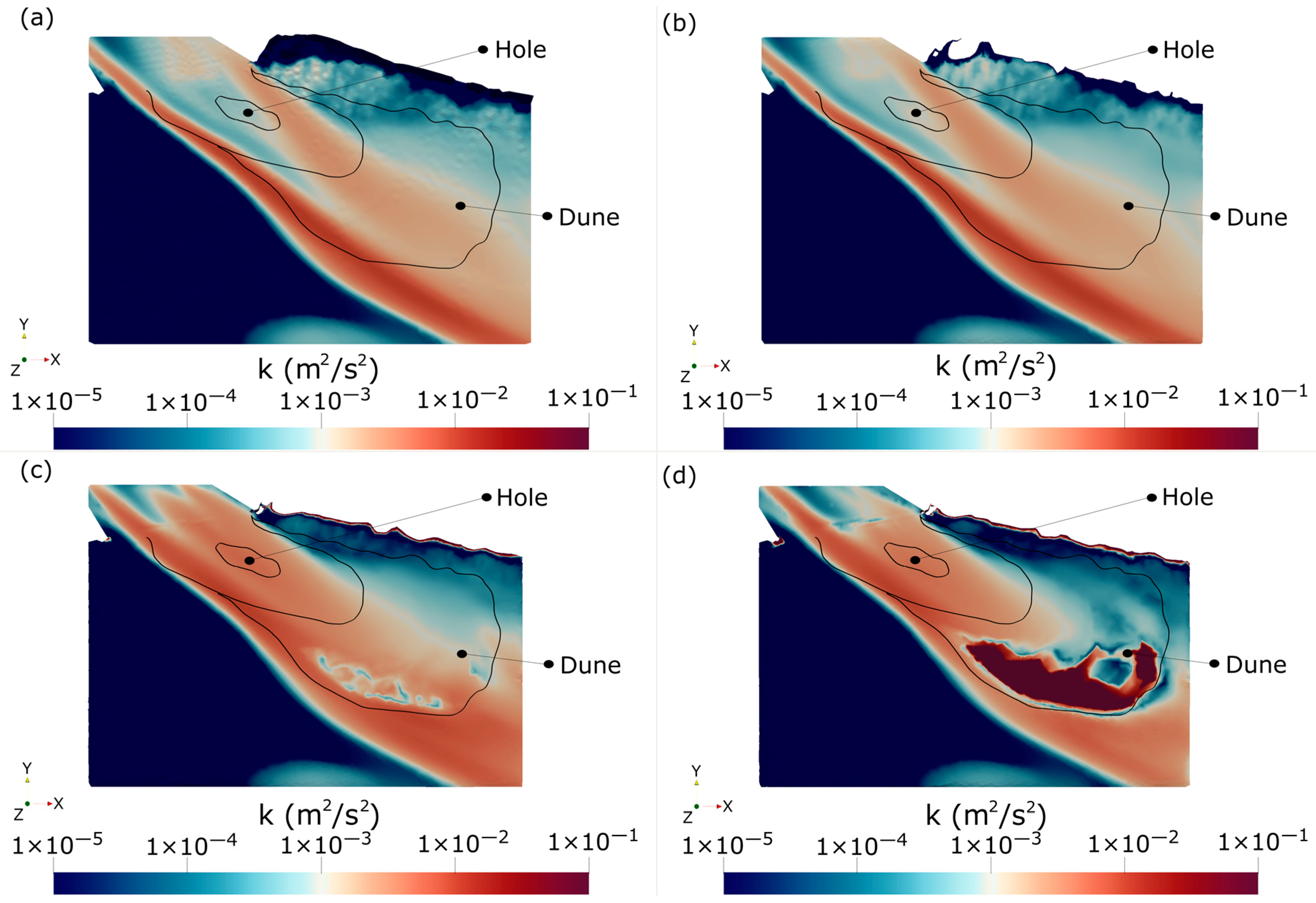
4.1. Scour Computed by the Numerical Model
4.2. Comparison with Empirical Formulas and Numerical Model Accuracy
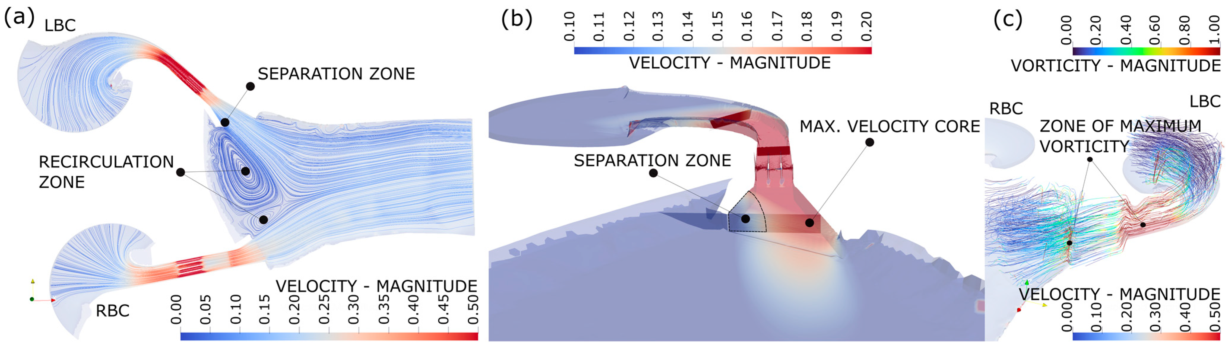
4.3. Comparison of Computed 2D vs. 3D Flow Structures
5. Conclusions
Author Contributions
Funding
Data Availability Statement
Acknowledgments
Conflicts of Interest
References
- Hoffmans, G.J.C.M.; Verheij, H.J. Scour Manual; Routledge: London, UK, 1997. [Google Scholar] [CrossRef]
- Garde, R.J.; Ranga Raju, K.G. Mechanics of Sediment Transportation and Alluvial Stream Problems/R.J. Garde, K.G. Ranga Raju, 3rd ed.; New Age International, Ed.; Daryaganj: New Delhi, India, 2015. [Google Scholar]
- Sousa, A.M.; Ribeiro, T.P. Local Scour at Complex Bridge Piers–Experimental Validation of Current Prediction Methods. ISH J. Hydraul. Eng. 2021, 27, 286–293. [Google Scholar] [CrossRef]
- Vanoni, V.A.; Brooks, N.H. Laboratory Studies of the Roughness and Suspended Load of Alluvial Streams; California Institute of Technology: Pasadena, CA, USA, 1957; p. E-68. [Google Scholar]
- Bombardelli, F.A.; Palermo, M.; Pagliara, S. Temporal Evolution of Jet Induced Scour Depth in Cohesionless Granular Beds and the Phenomenological Theory of Turbulence. Phys. Fluids 2018, 30, 085109. [Google Scholar] [CrossRef]
- Palermo, M.; Bombardelli, F.A.; Pagliara, S.; Kuroiwa, J. Time-Dependent Scour Processes on Granular Beds at Large Scale. Environ. Fluid Mech. 2021, 21, 791–816. [Google Scholar] [CrossRef]
- Zhao, P.; Yu, G.; Zhang, M. Local Scour on Noncohesive Beds by a Submerged Horizontal Circular Wall Jet. J. Hydraul. Eng. 2019, 145, 06019012. [Google Scholar] [CrossRef]
- Franzetti, S.; Radice, A.; Rebai, D.; Ballio, F. Clear Water Scour at Circular Piers: A New Formula Fitting Laboratory Data with Less Than 25% Deviation. J. Hydraul. Eng. 2022, 148, 04022021. [Google Scholar] [CrossRef]
- Ettema, R.; Constantinescu, G.; Melville, B.W. Flow-Field Complexity and Design Estimation of Pier-Scour Depth: Sixty Years since Laursen and Toch. J. Hydraul. Eng. 2017, 143, 03117006. [Google Scholar] [CrossRef]
- Lai, Y.G.; Liu, X.; Bombardelli, F.A.; Song, Y. Three-Dimensional Numerical Modeling of Local Scour: A State-of-the-Art Review and Perspective. J. Hydraul. Eng. 2022, 148, 03122002. [Google Scholar] [CrossRef]
- Castillo, L.G.; Castro, M.; Carrillo, J.M.; Hermosa, D.; Hidalgo, X.; Ortega, P. Experimental and Numerical Study of Scour Downstream Toachi Dam. In Sustainable Hydraulics in the Era of Global Change—Proceedings of the 4th European Congress of the International Association of Hydroenvironment Engineering and Research, IAHR 2016, Liege, Belgium, 27–29 July 2016; CRC Press: Boca Raton, FL, USA, 2016. [Google Scholar]
- Garfield, M.; Ettema, R. Effect of Clearwater Scour on the Flow Field at a Single Bendway Weir: Two-Dimensional Numerical Modeling Supported by Flume Data. J. Irrig. Drain. Eng. 2021, 147, 04021055. [Google Scholar] [CrossRef]
- Liao, C.T.; Yeh, K.C.; Lan, Y.C.; Jhong, R.K.; Jia, Y. Improving the 2d Numerical Simulations on Local Scour Hole around Spur Dikes. Water 2021, 13, 1462. [Google Scholar] [CrossRef]
- Jiménez, A. Calibración y Verificación de Las Leyes de Descarga de Una Estructura de Control; Instituto de Ingeniería, Universidad Nacional Autónoma de México: Mexico City, Mexico, 2017. [Google Scholar]
- ASTM C778-13; Standard Specification for Standard Sand. ASTM international: West Conshohocken, PA, USA, 2006.
- Hamdan, R.K.; Al-Adili, A.; Mohammed, T.A. Physical Modeling of the Scour Volume Upstream of a Slit Weir Using Uniform and Non-Uniform Mobile Beds. Water 2022, 14, 3273. [Google Scholar] [CrossRef]
- Nortek. The Comprehensive Manual for Velocimeters. Available online: https://www.nortekgroup.com/assets/software/N3015-030-Comprehensive-Manual-Velocimeters_1118.pdf (accessed on 28 May 2023).
- EDF-R&Da. Telemac-2D. User Manual. Version V8p2; 2020. Available online: http://www.opentelemac.org/index.php/manuals/viewcategory/8 (accessed on 28 May 2023).
- García, H.M. Sedimentation Engineering; Garcia, M., Ed.; MOP 110; American Society of Civil Engineers: Reston, VA, USA, 2008. [Google Scholar] [CrossRef]
- EDF-R&Db. Sisyphe. User Manual. Version V8p2; 2020. Available online: http://www.opentelemac.org/index.php/manuals/viewcategory/8 (accessed on 28 May 2023).
- Huybrechts, N.; Villaret, C.; Hervouet, J.M. Comparison between 2d and 3d Modelling of Sediment Transport: Application to the Dune Evolution. In Proceedings of the River Flow 2010: Proceedings of the International Conference on Fluvial, Braunschweig, Germany, 8–10 September 2010; Bundesanstalt für Wasserbau: Karlsruhe, Germany, 2010; pp. 887–893. [Google Scholar]
- Cao, Z.; Carling, P.A. Mathematical Modelling of Alluvial Rivers: Reality and Myth. Part 1: General Review. In Proceedings of the Institution of Civil Engineers—Water and Maritime Engineering; ICE Virtual Library: London, UK, 2002; Volume 154. [Google Scholar] [CrossRef]
- Finnie, J.; Donnell, B.; Letter, J.; Bernard, R.S. Secondary Flow Correction for Depth-Averaged Flow Calculations. J. Eng. Mech. 1996, 125, 848–863. [Google Scholar] [CrossRef]
- Knaapen, M.A.F.; Joustra, R. Morphological Acceleration Factor: Usability, Accuracy and Run Time Reductions. In Proceedings of the XIXth Telemac-Mascaret User Conference, Oxford, UK, 18–19 October 2012. [Google Scholar]
- Morgan, J.A.; Kumar, N.; Horner-Devine, A.R.; Ahrendt, S.; Istanbullouglu, E.; Bandaragoda, C. The Use of a Morphological Acceleration Factor in the Simulation of Large-Scale Fluvial Morphodynamics. Geomorphology 2020, 356, 107088. [Google Scholar] [CrossRef]
- Breusers, H.N.C.; Raudkivi, A.J. Scouring. In Dictionary Geotechnical Engineering/Wörterbuch GeoTechnik; Springer: Berlin/Heidelberg, Germany, 1991. [Google Scholar] [CrossRef]
- Breusers, H.C. Time Scale of Two Dimensional Local Scour. In Proceedings of the 12th Congress IAHR, Fort Collins, CO, USA, 11–14 September 1967; Volume 3. [Google Scholar]
- Farhoudi, J.; Smith, K.V.H. Time Scale for Scour Downstream of Hydraulic Jump. J. Hydraul. Div. 1982, 108, 1147–1162. [Google Scholar] [CrossRef]
- Negm, A.; Saleh, O.; Abdel-Aal, G.; Sauida, M. Investigating Scour Characteristics Downstream of Abruptly Enlarged Stilling Basins. In River Flow Proceedings of the International Conference on Fluvial Hydraulic; Didier Bousmar, Y.Z., Ed.; Balkema: Ghent, Belgium, 2002; pp. 1–1283. [Google Scholar]
- Dietz, J.W.W. Kolkbildung in Feinen Oder Leichten Sohlmaterialien bei Strömendem Abfluß. Bachelor‘s Thesis, Versuchsanstalt für Wasserbau und Kulturtechnik, Theodor-Rehbock-Flußbaulaboratorium, Universität Fridericiana Karlsruhe, Karlsruhe, Berenz, 1969. [Google Scholar]
- García Flores, M.; Maza Álvarez, J.A. Inicio de Movimiento y Acorazamiento. Capítulo 8 del Manual de Ingeniería de Ríos; Instituto de Ingeniería, Universidad Nacional Autónoma de México: Mexico City, Mexico, 1997. [Google Scholar]


| Section Scenario | S1 (%) | S1 (%) | S2 (%) | S2 (%) | S3 (%) | S3 (%) | General (%) | General (%) |
|---|---|---|---|---|---|---|---|---|
| A (without CFS) | 9.11 | 20.5 | 17.3 | 13.9 | 219 | 138.0 | 88.3 | 62.76 |
| B () | 7.55 | 30.4 | 24.7 | 20.2 | 45.4 | 57.6 | 24.7 | 40.4 |
| C () | 3.06 | 20.6 | 12.1 | 9.27 | 13.4 | 50.0 | 8.55 | 29.4 |
| Method | (cm) | Error |
| Experimental | 9.4 | - |
| Telemac2D-Sishype (MES) | 8.4 | 0.106 |
| Telemac2D-Sishype (MMS) | 43.2a | −3.6 |
| Breusers M1 (1967) | 7.64 | 0.187 |
| (1967) | 9.27 | 0.014 |
| (1967) | 9.44 | 0.004 |
| Farhoudi and Smith (1982) | 5.87 | 0.376 |
| Negm (2002) | 4.5 | 0.521 |
| Dietz (1969) | 6.48 | 0.311 |
Disclaimer/Publisher’s Note: The statements, opinions and data contained in all publications are solely those of the individual author(s) and contributor(s) and not of MDPI and/or the editor(s). MDPI and/or the editor(s) disclaim responsibility for any injury to people or property resulting from any ideas, methods, instructions or products referred to in the content. |
© 2023 by the authors. Licensee MDPI, Basel, Switzerland. This article is an open access article distributed under the terms and conditions of the Creative Commons Attribution (CC BY) license (https://creativecommons.org/licenses/by/4.0/).
Share and Cite
Caballero, C.; Mendoza, A.; Berezowsky, M.; Jiménez, A. Numerical–Experimental Study of Scour in the Discharge of a Channel: Case of the Carrizal River Hydraulic Control Structure, Tabasco, Mexico. Water 2023, 15, 2788. https://doi.org/10.3390/w15152788
Caballero C, Mendoza A, Berezowsky M, Jiménez A. Numerical–Experimental Study of Scour in the Discharge of a Channel: Case of the Carrizal River Hydraulic Control Structure, Tabasco, Mexico. Water. 2023; 15(15):2788. https://doi.org/10.3390/w15152788
Chicago/Turabian StyleCaballero, Christian, Alejandro Mendoza, Moisés Berezowsky, and Abel Jiménez. 2023. "Numerical–Experimental Study of Scour in the Discharge of a Channel: Case of the Carrizal River Hydraulic Control Structure, Tabasco, Mexico" Water 15, no. 15: 2788. https://doi.org/10.3390/w15152788
APA StyleCaballero, C., Mendoza, A., Berezowsky, M., & Jiménez, A. (2023). Numerical–Experimental Study of Scour in the Discharge of a Channel: Case of the Carrizal River Hydraulic Control Structure, Tabasco, Mexico. Water, 15(15), 2788. https://doi.org/10.3390/w15152788