Simulation and Prediction Algorithm for the Whole Process of Debris Flow Based on Multiple Data Integration

Abstract

In order to solve the problems of large errors and low accuracy in debris-flow forecasting, the simulation and prediction algorithm for the whole process of debris flow based on multiple data integrations is studied. The middleware method is used to integrate multiple GIS data sets, and the GIS spatial database after multiple data integrations is used to provide the basis of data for the whole process simulation and prediction of debris flow. The spatial cellular simulation model of debris flow is built using the cellular automatic mechanism. The improved kernel principal component analysis method is used to reduce the dimension of debris-flow prediction index data. The reduced dimension index data is input into the support vector machine, and the support vector machine is used to output the prediction results of debris flow in the space cell simulation model of debris flow. Through the simulation visualization technology, the dynamic display of the simulation prediction of the whole process of debris flow is carried out. The experimental results show that the algorithm can realize the simulation of the whole process of debris-flow changes, that the prediction results of debris flow are close to the actual results, and that the error is less than 5%, which improves the prediction accuracy of debris flow and can be used as the auxiliary basis for relevant decision-making departments.

1. Introduction

The advent of the Internet and big data era has brought unprecedented opportunities for disaster prevention, especially in the field of geological disasters. As one of the most common geological disasters [1], debris flows have attracted extensive attention in China and even around the world. China is a country with complex mountains and landforms and subject to frequent geological disasters. As one of the most common geological disasters, debris flows have aroused widespread concern and attention in China and even around the world. The state and government departments use various methods to prevent debris-flow disasters, but debris flows are a complex nonlinear system [2] with great uncertainty. The formation of debris-flow disasters is the comprehensive result of various natural and human factors and the comprehensive result of the natural rainfall system acting on the surface geological environment system [3], which directly threatens. Debris flows cause great harm to the world and China every year. Debris flows have great destructive power, which seriously threatens the lives, safety, and property of residents near and on mountains and restricts the rapid development of the local economy. Because debris flows often occur under the conditions of a rainstorm or long-term continuous rainfall [4], their occurrence is seasonal and cyclical. The most economical and effective way to reduce debris-flow hazards is by mastering the occurrence law of debris flows [5], then accurately predicting the occurrence time and reasonably selecting the opportunity to avoid debris flows. As an important and scientific means of disaster prevention, the early warning of debris flows has attracted the close attention of relevant scholars at home and abroad as it is an important and difficult topic in debris-flow research. As an important and non-engineering measure for disaster prevention and mitigation [6], the early warning of debris flows involves the accurate and timely release of early warning information; taking preventive measures; ensuring the safety of people’s lives and property; and achieving the purpose of disaster prevention and mitigation by predicting its occurrence, location, level, scale, threat scope, and risk degree. It is very necessary to adopt scientific and advanced debris-flow prediction methods, establish an effective prediction system, improve its prediction accuracy, carry out active and effective prediction research [7]. As a new measure to prevent disasters, if the prediction system of this study were to be successfully developed and applied, it can realize the real-time and automatic early warning of debris-flow disasters, new ways of information monitoring, information transmission, information processing, etc., by combining early warning technology with current advanced science and technology, thereby reducing the social impact and economic losses caused by debris-flow disasters. It can also provide a scientific basis for government departments to formulate disaster prevention plans, issue early warning information, and reasonably plan regional economic development. Debris-flow disasters can adopt characteristics suddenly, and there are no obvious signs before this occurs. The duration is relatively short, but the destructive power is extremely strong [8]. They very easily cause casualties and property losses. The accurate prediction of debris-flow disasters can reduce or even avoid casualties. At present, it is also one of the most important means of disaster reduction and prevention of debris-flow disasters. The prediction of debris-flow disasters has always been one of the focuses of scholars from relevant departments around the world. A debris-flow disaster is a kind of natural disaster that causes great harm, so it is very necessary to make accurate predictions and trend predictions for it.

The geographic information system (GIS) is a system often used in various fields at present. Applying GIS technology to debris-flow prediction will provide spatial data for debris-flow prediction, which will improve the prediction performance. Data are an important part of GIS, and the acquisition of spatial data plays an important role. In fact, the whole GIS is developed around the collection, processing, storage, analysis, and presentation of spatial data. In order to make full use of the existing data [9], reduce costs, and realize the sharing of informational resources in the process of project implementation, it is often necessary to use various spatial data from different sources, such as survey data, remote sensing data, etc. In addition, due to the diversity of GIS software, each one has its own specific data model, resulting in different data storage formats and structures. In the process of using GIS data, due to different data sources, structures, and formats, certain technical methods need to be adopted to combine them [10], which leads to the problem of multiple data integration. With the development and application of the Internet, it has become an urgent problem that various data can be directly integrated and accessed by the system. At present, most application systems use special data conversion tools to achieve data integration. In debris-flow prediction, the GIS that collects multiple data sets is required to be able to directly integrate, access, and process data in different formats due to the diversity of software and data sources [11] as well as integrate data in different formats and from different sources into the spatial data applied to debris-flow prediction. The integration performance of multiple data sets is extremely important.

There have been many scholars studying debris-flow prediction. Banihabib et al. used an artificial intelligence model to overcome the shortcomings in the impact of sediment concentration on debris flow [12] since sediment concentration is an effective factor that can be used to evaluate the peak flow of debris flow. The proposed artificial intelligence model is used to estimate the sediment concentration of floods, and the average watershed elevation, average watershed slope, watershed area, daily rainfall, and early rainfall are specified to achieve an effective prediction of debris flow. Kováík et al. used the local method of weighted square to establish the debris-flow model [13]. When building the debris-flow model, they focused on the establishment of a dry granular soil movement model and used the constructed debris-flow model to achieve an effective prediction of debris flow. Debelak et al. built a three-dimensional finite element model for the stress displacement behavior of the flexible debris-flow mitigation structure [14] and simulated the coupling behavior encountered in the flexible debris-flow mitigation structure by using the flexible steel-ring network structure for debris-flow mitigation in mountainous terrain. The debris-flow is modeled as a series of rectangular solid blocks, and the flexible debris-flow barrier is modeled as a series of rings, cables, and braking elements. Moreno E et al. used the mixed stable finite element method to numerically simulate debris-flow [15]. The location of the flowing free surface was determined using a mixed stable velocity/pressure finite element formula. By using orthogonal subgrid-scale stabilization (OSS) and segmented orthogonal subgrid-scale stabilization techniques, the equal order interpolation of the velocity and pressure was achieved. The dual-viscosity-regularized Bingham model was introduced to track and predict the movement trend of the free surface of debris flow. Viktoriia K et al. calculated the scale of debris flow based on the simulation and prediction of debris-flow protection structures [16]. The modeling of unstable water motion was conducted. During the modeling process, five possibilities of debris-flow occurrence were predicted based on the maximum flow of nearby rivers. Yan Y et al. studied a data-driven, multi-objective evolutionary optimization method for debris-flow prediction [17]. The Pareto optimality method is used to quantify nonlinear and conflicting critical rainfall thresholds. The combination of artificial neural network and particle swarm optimization for multi-objective evolutionary optimization is used to achieve debris-flow prediction. Although the above methods can predict debris flow, the impact of multiple data sets on the prediction accuracy of debris flow is not considered, resulting in a certain deviation between the prediction results of debris flow and the actual debris flow. In order to solve the problem of low accuracy in debris-flow prediction using the above methods, the simulation and prediction algorithms of the whole process of debris flow under the integration of multiple data sets are studied by integrating multiple data for debris-flow prediction with middleware data from GIS software, innovatively utilizing the three-level cellular automation mechanism of initializing cell states, regularly scanning and updating, and incorporating unit-level response processes to construct a full process simulation model for debris-flow prediction. The identification of debris flow is based on indicators such as cardinality, slope, and soil texture in the debris-flow prediction index system, and support vector machines are selected to output the prediction results of debris flow. This method has good prediction ability, which is useful in debris-flow disaster prediction, and provides a new idea for debris-flow disaster prediction and control.

2. Simulation and Prediction of the Whole Process of Debris Flow Based on Multiple Data Integration

2.1. Multi-Source Data Integration Method of Debris-Flow Prediction GIS Based on Middleware

2.1.1. Multi-Source Data Integration Structure Based on Data Middleware Mode

Automatically collect and integrate multi-source data for debris-flow prediction using middleware. Middleware is an independent system software or service program that can automate data collection and integration. Distributed application software uses this software to share resources between different technologies. Middleware is located in the operating system of the client server to manage computing resources and network communication. Middleware can generally be understood as a reusable basic software layer between the operating system and application software. Middleware is a relatively broad concept; from a small component on a single machine to a complex enterprise application server, it can be regarded as a category of middleware.

The concept of middleware is used to define GIS data middleware to solve the seamless integration of GIS multi-source spatial data. The so-called GIS data middleware refers to software plug-ins that can be embedded into various GISs. These plug-ins are independently completed by various GIS software developers and users. Its principle is similar to the driver design of plug-and-play devices, that is, the developers of the GIS software platform specify the read–write interfaces of the internal data of the system. These interfaces operate within the platform or exchange data structures. For spatial data from different sources, including the relative height difference, soil texture, erosion intensity, formation lithology, disaster sensitivity, 24 h of rainfall, the maximum hourly rainfall and other data, the data provider writes the operation code in the internal data read–write interface. After compilation and registration, the GIS software platform can operate such spatial data. The structure diagram for realizing multiple data integrations for debris-flow prediction using middleware is shown in Figure 1.

As shown in Figure 1, the task of GIS data middleware is completed in two stages over a period of time. In the first stage, a certain type of GIS software developer specifies the data input/output (I/O)interface of the GIS data middleware according to the characteristics of this type of GIS and completes the corresponding part that directly communicates with the bottom layer of the GIS. In the second stage, GIS users complete the data source interpretation part of the middleware according to their own needs and the characteristics of the spatial data source they are dealing with. After a simple compilation, the operable GIS data middleware is implemented and registered into the system. Then, the GIS will complete the support of users’ multiple data sets. The spatial database of the GIS, after multiple data integrations, is used to provide the basis of data for the simulation and prediction of the whole debris-flow process.

2.1.2. Realization of GIS Multiple Data Integration for Debris-Flow Prediction

GIS multiple data mainly consists of internal data writing API, middleware interface data, and user middleware data. The internal data written to the API are provided by the kernel, which converts the parameters through the API into the standard data structure of the kernel. The data middleware interface mainly specifies the user data interpretation entry. After the interface content is completed, compile and connect it as a dynamic connection library, copy it to the data middleware directory of the kernel, register it in the system, and complete the data collection process of user middleware. Using data middleware technology, the tasks of developers and data providers are clear. Through the designed data middleware interface, spatial data provided by different types of GISs is received through different data middleware. In order to complete the loading of multi-source spatial data quickly and in parallel, it is necessary to integrate multiple data sets through spatial mapping after receiving data.

Based on the state space method, the information fusion integration is regarded as the mapping process from the external space to the target space. Set the GIS environment space as $H$, and middleware interface data space as $B$.

The target spatial data for prediction data is expressed as

$$H=\left[\begin{array}{l}{H}_{11}\hspace{1em}{H}_{12}\hspace{1em}\cdots \hspace{1em}{H}_{1n}\\ H_{21}\hspace{1em}{H}_{22}\hspace{1em}\cdots \hspace{1em}{H}_{2n}\\ ⋮\hspace{1em}\hspace{1em}⋮\hspace{1em} ⋮\hspace{1em}\hspace{1em}⋮\\ H_{m1}\hspace{1em}{H}_{m2} \cdots \hspace{1em}{H}_{mn}\end{array}\right]$$

(1)

where $H_{mn}$ represents debris-flow prediction target space the goals of $m$ and the elements of $n$.

The middleware interface data space is $B$ and is described as:

$$B=\left[\begin{array}{l}{B}_{11}\hspace{1em}{B}_{12}\hspace{1em}\cdots \hspace{1em}{B}_{1h}\\ B_{21}\hspace{1em}{B}_{22}\hspace{1em}\cdots \hspace{1em}{B}_{2h}\\ ⋮\hspace{1em}\hspace{1em}⋮\hspace{1em} ⋮\hspace{1em}\hspace{1em}⋮\\ B_{g1}\hspace{1em}{B}_{g2}\hspace{1em}\cdots \hspace{1em}{B}_{gh}\end{array}\right]$$

(2)

where $g$ indicates the type and quantity of debris-flow monitoring data, and $h$ is the maximum number of middleware interfaces.

Using fuzzy rules, construct the GIS environment space for the mapping association for $H$ and $B$:

$${\lambda }_{HB}=\frac{{\displaystyle \sum B{\phi }^{gh}}}{{\displaystyle \sum _{}H{w}_n^m}}$$

(3)

Here, ${\phi }^{gh}$ express the spatial data mapping confidence of $B$, and $w_n^m$ is the membership degree of spatial data of $H$.

The fusion result of the two spaces is obtained by mapping the trust function.

$$G=J{{\displaystyle \sum \left({\lambda }_{HB}{t}_n\right)}}^q$$

(4)

Here, $J$ represents the trust function of fuzzy rules, $q$ represents the maximum amount of data that can be obtained by fusion, and $t_n$ represents the interval of times for data access of $n$ time.

Therefore, the integration of multiple data from a debris-flow prediction GIS is realized. The integrated data is used to build the debris-flow simulation model.

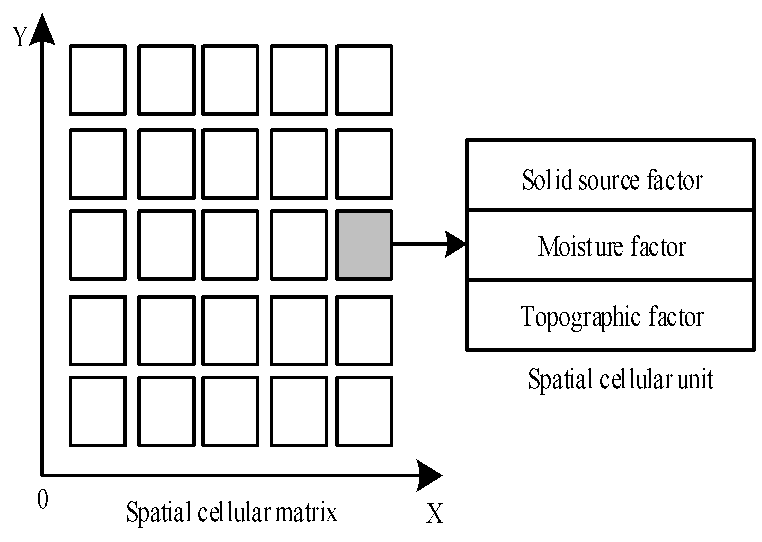
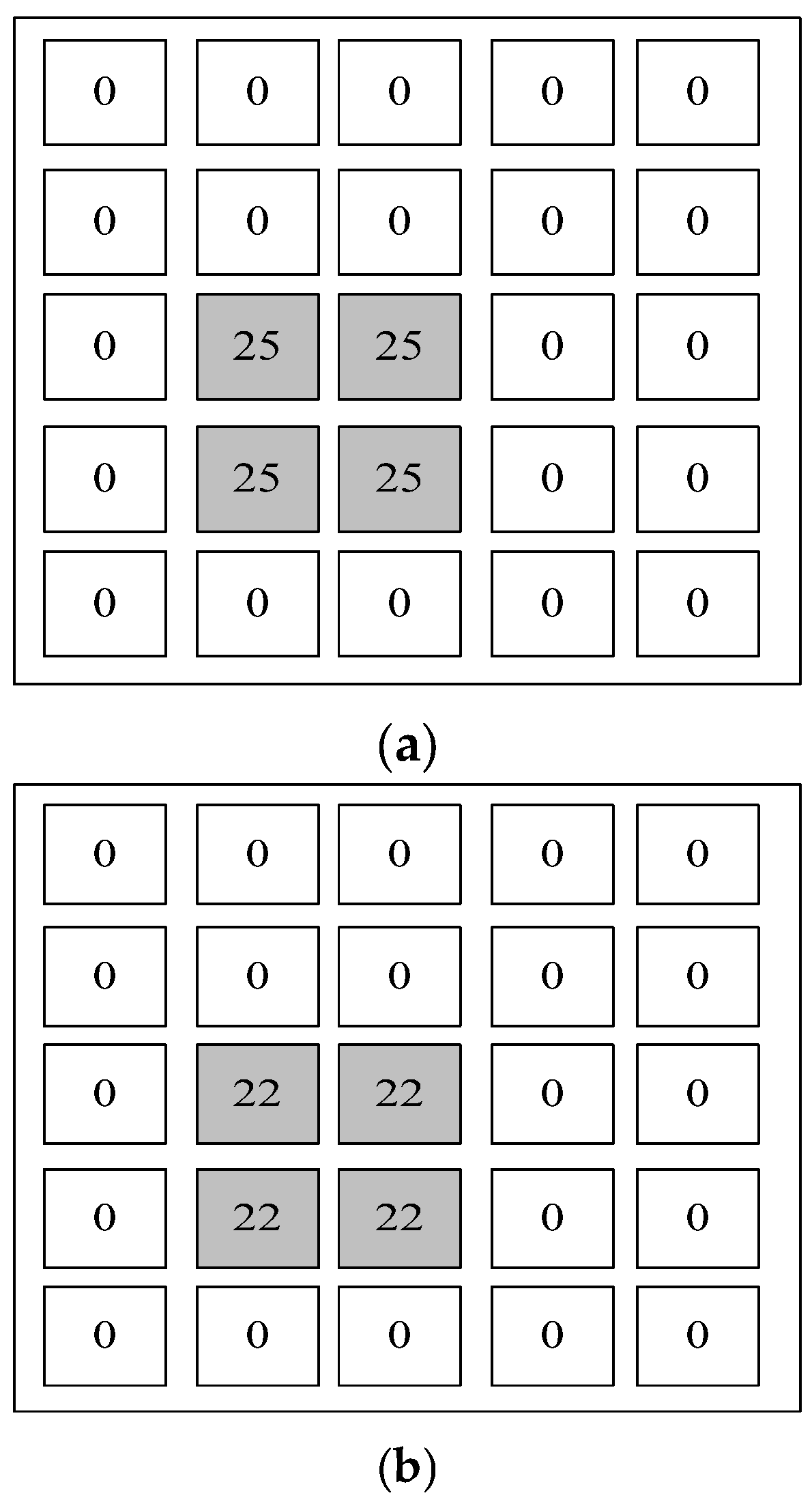
2.2. Construction of Spatial Cell Simulation Model of Debris Flow

Based on the GIS multi-source fusion data for debris-flow prediction obtained in the previous section, the space cell simulation model of debris flow is built using the cellular automatic mechanism. In the space cell simulation model, the whole process of debris-flow simulation prediction is carried out.

The composition expression of cellular automata is as follows:

$$A=\left(L,d,S,N,f\right)$$

(5)

In Formula (5), $A$ is the cellular automata, $L$ is the cell space, $d$ is the dimension of the cell space, $S$ is a set of states with finite and discrete cells, $N$ is the collection of all cells in a certain field, and $f$ is the updated rules for cell status. The core elements of the above five elements are $S$ (state set) and $f$ (cell-state update rules). Different objects have different characteristics, application backgrounds, and materialization theory laws. When constructing the spatial cell model of debris flow, it is necessary to customize different status attribute groups and status update rules according to debris flow so as to ensure that the model can simulate debris-flow objects as truly, objectively, and ideally as possible [18]. The precise definition of model static attributes and dynamic updating rules needs to be based on solid debris-flow theory. Based on the spatial cell simulation model of debris flow, a systematic and complete spatial cell model describing the movement process of debris flow is established.

The schematic diagram of the spatial cell simulation model of debris flow is shown in Figure 2.

Figure 2 shows that the spatial dimension and structure of the model use a two-dimensional square-grid structure. The reason why the spatial unit model is adopted in this paper is that each cell in the model has the ability to interact with adjacent cells. By repeating the rules of local cells, the dynamic simulation of debris flow in the whole space can be realized, which lays a good foundation for the accurate dynamic prediction results of the following section so as not to be disturbed by the influencing factors.

Zoom in to observe a specific cell in the space cell matrix; a specific cell is referred to as a “cell cube”. It mainly includes four categories of attribute data, namely terrain attribute data, solid source attribute data, rainfall attribute data, and motion model attribute data. These data are stored in the cell cube element, which simulates the real environment of the earth’s surface discretely. The different morphological combinations of the data sets in the entire spatial cell matrix constitute a finite and discrete state set in the spatial cell model.

When the static state set is clearly defined by all attributes, it is necessary to discuss how to generate the dynamically changing spatial-cell-state update rules. The spatial cell state of debris flow is set as follows:

(1) Initialize cell state

When the model is first being established, the space cell initializes all attribute states according to the actual conditions of the objects in the simulation area. The attribute data here is a discrete numerical simulation of the objective real world, and its accuracy depends on the spatial resolution set by the cell [19]. Under the condition of different data source precision, an interpolation operation or other measures are required to assimilate the data source to the same resolution.

(2) Periodic Scan Update

In order to facilitate the computer algorithm processing the overall scale of the spatial cell matrix, the periodic progressive scanning mode for state update is adopted [20]. That is, for each cell in the spatial cell matrix, the state update operation at the cell level is implemented from the top left corner to the right. At the time of $t$, using cell $\left(i,j\right)$, the space spread function completes the status update calculation.

$$Z_{i,j}^t=A\left(\frac{G_t}{G_0},t\right)$$

(6)

In Formula (6), $G_t$ and $G_0$, respectively, represent the amount of time $t$ that the water was being produced by rainfall for the spread of debris-flow cells and the amount of water required to trigger debris flow. When the calculation reaches the end of the line, it starts from the leftmost cell of the next line and sweeps from left to right again until the last cell of the lower right corner of the matrix, ending the cycle of state update calculations.

(3) Cell-Level Response Flow

In fact, the dynamic simulation of the spatial cell model is realized by each spatial cell unit at the bottom based on the same “evolution” rules, making their own independent and interactive responses in each time step. Similar to the grid spatial data format, the pixel matrix is used to express spatial entities, but it is more complex and dynamic. The response process definition of a cell unit is one of the core parts of the modeling of the whole spatial cell model. The priority of the rainfall attribute treatment is better than that of the solid source attribute treatment, because it provides some preconditions that need to be involved in the latter treatment process. There are tow sources of current cell surface water: (1) existing surface water and rainfall data within the current time step, through which specific objects in the whole rainfall attribute processing can be identified. (2) To judge whether there are seepage conditions, when the calculation enters the process module of rainfall attribute processing, the current surface water permeability needs to be calculated:

$$n=\frac{Z_{i,j}^t\left(a^{\prime }+b^{\prime }\right)}{a^{\prime }+\frac{b^{\prime }}{\rho }}\left(1-c^{\prime }\right)$$

(7)

In Formula (7), $a^{\prime }$ and $b^{\prime }$, respectively, represent the proportion of existing surface water and rainfall in the solid source unit in the current time step; $c^{\prime }$ indicates the proportion of current flow water in the overall unit of debris-flow initiation, and $\rho$ is the velocity coefficient of flow spread.

If the permeability is not zero, the current surface water shall be infiltrated according to the permeability. There may be two situations that lead to a random judgment error with zero permeability: the current solid source is already in a water-saturated state or it cannot absorb any more water. At present, the solid source, which is the main component of debris flow, has moved as a whole with the beginning of the debris flow, and the permeability here is basically close to zero. In order to control the error caused by this error, the absorption part of the solid material source is removed from the current surface water, and the remaining part is determined as flowing water, which will be distributed according to the elevation of the adjacent 8 cells and the current unit. Retrieve the elevation of adjacent 8 cells, and if it is lower than the current cell elevation, add it to the stream target cell queue. Check the flow destination queue. If it is zero, there is no flow, and this part of the water is trapped. If it is not zero, the water is flowing. After completing the allocation of surface runoff, the rainfall attribute processing was completed to avoid judgment errors with zero permeability. The processing process for solid source attributes is as follows:

(1) It is necessary to judge whether there is a solid material source plate that can participate in debris-flow activities in the cell unit. If there is one, the process will continue. If not, it will jump out and end the solid material source treatment process.

(2) Calculation of external force components. If there is a migration of solid material sources in the adjacent eight space cells, it will inevitably exert a force on the next space cell in the migration direction, which may cause a chain domino effect. Therefore, this step carries out the vector superposition of all possible forces in the eight directions, in order to obtain a comprehensive external force.

(3) Judge whether there is a solid source migrating into the current space cell. If there is no solid source, the process will continue to jump to the next step. If there is a solid source, it needs to be fused.

(4) For the migration of solid material source, determine whether there is a target unit that will not be migrated in the adjacent 8 units. The basis for the preliminary judgment here is the elevation difference, that is, whether there is an elevation lower than the current space cell in the adjacent unit. If there is an elevation lower than the current space cell, conduct a more specific stress analysis. If not, jump out and end the processing process. The process of force analysis is the process of comparing the maximum static friction force and sliding force on the solid source plate on the slope formed by each pair of current space cells and target space cells. If the sliding force is greater than the maximum static friction force, the migration starting condition is met. In the end, the solid material source will migrate in the direction with the largest sliding trend, and the migration target space cells will be marked. Through the simulation visualization technology, the dynamic display of the simulation prediction of the whole debris-flow process will be carried out.

2.3. Prediction Algorithm for the Whole Process of Debris Flow

2.3.1. Establishment of Debris-Flow Prediction Index System

The simulation model established in the previous section is used to simulate the whole process of debris flow, and the probability of its occurrence is predicted based on the prediction index. The formation of debris flow is a complex process, which requires favorable terrain conditions, material source conditions and hydrodynamic conditions at the same time. The relative height of the slope, slope gradient, vegetation coverage, soil texture, stratum lithology, erosion intensity, loose material reserves of the slope, disaster-sensitive zones, accumulated rainfall in the first 7 days, 24 h rainfall, and maximum hourly rainfall are selected as the impact indicators of the debris-flow prediction model. Among them, the reserves of loose slope materials are an important source of debris flow. The larger the reserves are, the more solid debris can be provided when debris flow occurs. The looser the solid debris is, the easier it is to lose stability and to cause damage under rainfall conditions. Therefore, the loose materials in debris-flow gullies have certain reserves, which provide the source conditions for the formation of debris flow. The slope gradient reflects the stability and hydrodynamic conditions of soil particles on the slope, and directly affects the scouring and transportation capacity of surface runoff. The vegetation coverage index reflects the ability to prevent water and soil loss. The higher the coverage rate, the greater the energy required for rock and soil mass instability. The relative elevation difference of the slope reflects the terrain conditions of the valley. The greater the elevation difference, the greater the potential energy provided, the stronger the hydrodynamic force, and the greater the possibility of debris flow. The maximum hourly rainfall is an important starting factor for debris flow. The greater the intensity, the higher the possibility of rock and soil mass instability, and the greater the possibility of debris flow outbreak; 24 h rainfall refers to the rainfall 24 h before this time. The greater the rainfall, the greater the possibility of debris flow. The amount of accumulated rainfall in the early stage reflects the degree of saturated liquefaction of the soil to a certain extent. According to the impact of early rainfall, when debris flow occurs, the accumulated rainfall of 7 days is selected as the impact index of early rainfall. After the determination of debris-flow prediction indicators, these indicators are divided into three layers: the target layer, criterion layer and indicator layer. The criterion layer is divided into three parts, namely, the basic factor, response factor, and induction factor. The debris-flow prediction index system is shown in

Table 1. Prediction index system of debris flow.

Target Layer	Criterion Layer	Index Layer
Debris-flow prediction	Base factor	Relative height difference
		Slope grade
		Soil texture
		Vegetation coverage
		Erosion intensity
		Stratigraphic lithology
	Response factor	Mass of loose material in slope
		Disaster sensitivity
	Inducible factor	Rainfall in the first 7 days
		24 h rainfall
		Maximum hourly rainfall

.

The obtained debris-flow prediction index data are complex and difficult to be quantified and evaluated uniformly, so it needs to be reduced and normalized.

2.3.2. Dimension Reduction in Debris-Flow Prediction Index Data Based on Improved Kernel Principal Component Analysis

The improved kernel principal component analysis method is used to reduce the dimension of the debris-flow prediction index data in the previous section. Kernel principal component analysis is a method of data dimensionality reduction and feature extraction. Its basic idea is to use the kernel function to convert the nonlinear correlation of the initial principal component analysis index data into a linear correlation and perform principal component analysis in the mapped kernel function space. In order to ensure the high rationality of the data in practical applications and to effectively reduce data dimensions and extract features, the traditional kernel principal component analysis method is improved. The improved kernel principal component analysis method is obtained by introducing the idea of weight values in the covariance matrix and influencing the weight of samples or features in the original data in the model.

Set the training sample set of debris flow whole-process prediction indicators as $X=\left\{x_1,x_2,\cdots ,x_n\right\}$, where $x_i\in R^p$, $y_i=R^p$, $R^p$ represents the input space, and $p$ indicates the index dimension. For the nonlinear mapping in input space $\phi :X\to F$, $F$ represents the characteristic space of the whole debris-flow prediction.

Introduce weight idea into covariance matrix $G$. The construction expression is as follows:

$$G=\frac{1}{n}{\displaystyle \sum _{i=1}^n{h}_i}\cdot \phi \left(x_i\right){\phi }^T\left(x_i\right)$$

(8)

In Formula (2), $G$ is the covariance matrix, $n$ is the number of training samples, $\phi \left(\cdot \right)$ is the nonlinear mapping of the input space, and $h_i$ is the feature weight, so that $w_i=\sqrt{h_i}$, thereby meeting the standardized range of weight ${\displaystyle \sum _{i=1}^n{h}_i}\phi \left(x_i\right)=0$.

The eigenvector expression of the whole debris-flow prediction is obtained as follows:

$$v_r={\displaystyle \sum _{i=1}^{n}G{w}_i}\phi \left(x_i\right)$$

(9)

Because the eigenvector $v$ is composed of nonlinear mapping space, selecting $m$ normalized eigenvector corresponding to eigenvalues $a_1,a_2,\cdots ,a_m$ results in the projection expression of $\phi \left(x_j\right)$ to $v_r$ is as follows:

$$g_r\left(x_j\right)=\phi \left(x_j\right)\cdot v_r={\displaystyle \sum _{i=1}^n{a}_m^{}\left(w_i\phi \left(x_i\right)\cdot w_i\phi \left(x_j\right)\right)}$$

(10)

In formula (6), $g_r\left(x_j\right)$ is of the $r$ nonlinear principal component corresponding to $\phi \left(x\right)$.

Make all projected values $g\left(x_j\right)$ as the characteristic sample of the whole-process prediction of debris flow. The kernel function is used to replace the calculation of spatial point product, and Formula (11) is converted as follows:

$$g\left(x_j\right)=\phi \left(x_j\cdot v_r\right)={\displaystyle \sum _{i=1}^n{a}_r^{i}K\left(w_i{x}_i,w_i{x}_j\right)}$$

(11)

Using the eigenvalue, the individual contribution rate of the prediction index of the whole debris-flow process is calculated as follows:

$$Z=\phi \left(x\right)/{\displaystyle \sum _{}^{}g\left(x_j\right)}$$

(12)

The influence factors of the principal components of debris-flow prediction are calculated according to the characteristic values, and the cumulative contribution rate is defined as ≥85%, for the selected principal component factors of $b$ applied to debris-flow prediction.

2.3.3. Prediction Algorithm of Debris Flow Based on Support Vector Machine

Set the index data obtained after the dimension reduction processing of the index data in the previous section as the input of the support vector machine, and use the support vector machine to output the debris-flow prediction results. A support vector machine is developed from the optimal classification surface in the case of simple linear separability. The support vector machine is selected as the algorithm for the simulation and prediction of the whole debris-flow process. There is a two class linearly separable sample set of debris-flow prediction data $\left(x_i,y_i\right),x\in R^d,y\in \left\{1,-1\right\}$, using $w$ to represent the weight value. At this time, the classification interval is equal to $2/‖w‖$, with an minimum interval of up to ${‖w‖}^2$. Send $\frac{1}{2}{‖w‖}^2$. The smallest classification plane is the optimal classification plane of the support vector machine, and the points on the optimal classification plane are called support vectors. The optimal classification surface problem can be expressed as a constrained optimization problem, and the minimum value of the following functions can be obtained:

$$\varphi \left(w\right)=\frac{1}{2}{‖w‖}^2$$

(13)

While introducing Lagrange multipliers $a_i$, transform the above optimal classification surface problem into a dual problem, that is, set ${\displaystyle \sum _{i=1}^n{a}_i}{y}_i=0\hspace{1em}$. With constraints on $a_i$, solve the objective function and the maximum value of $Q\left(a\right)$, where the expression of $Q\left(a\right)$ is as follows:

$$Q\left(a\right)=\varphi \left(w\right){\displaystyle \sum _{i=1}^n{\displaystyle \sum _{j=1}^{n}bZ{a}_i}}\left(x_i\cdot y_i\right)$$

(14)

Using the above process, the optimal classification surface function expression of debris-flow prediction is constructed as follows:

$$f\left(x\right)=sng\left\{\left(x\cdot w\right)+Q\left(a\right)\right\}=sng\left\{{\displaystyle \sum _{i=1}^n{a}_i^{}{y}_i}\left(x\cdot w\right)\right\}$$

(15)

Debris-flow prediction is a nonlinear classification problem, which is transformed into a linear problem in high-dimensional space through nonlinear transformation, and the optimal classification surface is found in the transformation space. Support vector machines use kernels to solve complex nonlinear and linear problems. When introducing the kernel function $K\left(x_i,x_j\right)$, the objective function expression of debris-flow prediction probability is then constructed as follows:

$$Q{\left(a\right)}^{\prime }={\displaystyle \sum _{i=1}^{n}f\left(x\right)}-\frac{1}{2}{\displaystyle \sum _{i=1}^n{\displaystyle \sum _{j=1}^n{a}_i}}K\left(x_i\cdot y_i\right)$$

(16)

Use Formula (16) to output the prediction result of debris flow, and the output value of the prediction result of debris flow is the probability result of debris-flow occurrence. Therefore, the simulation and prediction of the whole debris-flow process based on multiple data integration is complete.

3. Results and Discussions

In order to verify the effectiveness of the debris-flow whole-process simulation prediction algorithm based on multiple data integration, a railway section in the mountainous area of southwest China was selected as the test object for debris-flow prediction. The section is located near Seda County, Ganzi Prefecture, Sichuan Province, China. This section is an important transportation trunk line, with complex geological conditions, steep terrain along the line, and frequent geological disasters. There are 158 large landslides, nearly 450 dangerous rocks, 235 debris-flow ditches, more than 190 rock piles, and more than 100 collapses along the railway. Under the control of topographic factors and the influence of fault structures, debris-flow disasters occur frequently in this section. Using this section as a debris-flow prediction area not only strengthens the monitoring and risk management of the area, but also provides a large amount of data, which is required for the simulation and prediction of debris flows under complex geological conditions, including geological terrain data, rainfall data, soil moisture data, etc. There are more than 100 debris-flow gullies of different sizes along the railway in this section. Debris-flow gullies are widely distributed and numerous, with different levels of harmfulness and great changes in geological conditions. Therefore, it is urgent to apply the prediction algorithm for debris-flow risk suitable for the special geological conditions in the section to timely predict the existing and newly developed debris flows in the section.

The method described in this paper is used to integrate GIS multiple data with middleware, build the GIS spatial database, and utilize the data in the GIS spatial database to provide the basis of data for debris-flow prediction. This method is used to obtain the geographical environment map of the debris-flow prediction area from GIS software, as shown in Figure 3.

Through an analysis of the experimental results in Figure 3, it is clear that this method effectively integrates the data of various indicators of debris-flow prediction from different software and obtains different types of data, such as terrain data related to the study area. The integrated GIS spatial database is used to provide data on various indicators for debris-flow prediction. In order to prevent overfitting, a small data set was set up in the model training, and the various index data were divided into the training set and test set in a 7:3 ratio.

The method in this paper is used to reduce the dimension of the debris-flow prediction index system by using the nuclear principal component analysis method. The values of each prediction index in the study area after the dimension reduction are collected, and the collected index values are normalized. The normalized processing results of the debris-flow prediction index are shown in

Table 2. Normalized processing results of debris-flow prediction indexes.

Index Name	Normalized Results
Relative height difference	0.852
Soil texture	0.751
Erosion intensity	0.254
Stratigraphic lithology	0.162
Disaster sensitivity	0.284
24 h rainfall	0.394
Maximum hourly rainfall	0.584

.

It can be seen from the experimental results in Table 2 that 11 indicators of the debris-flow prediction indicator system are dimensionally reduced by using the nuclear principal component analysis method. After a dimensionality reduction, a total of seven indicators related to debris-flow prediction are determined. By normalizing the debris-flow prediction indexes after dimension reduction, the data input into the support vector machine for debris-flow prediction is obtained.

After the test data is prepared, ArcGIS software is used to conduct a numerical simulation of the debris flow’s rushing range and hazards, and the global simulation operation is carried out step by step according to the time step. During each global simulation operation, the numerical state of each layer of the spatial cell matrix after a time step should be observed, recorded, and saved. The dynamic change results of the solid-matter source layer, solid-matter source-absorption water layer, and runoff layer predicted by the test are shown in Figure 4.

It can be seen from the experimental results in Figure 4 that the full process change of debris flow can be simulated by using the space cell simulation model built by the cell automatic mechanism in this method, and the dynamic change of the whole process of debris flow can be simulated through the simulation of the solid source layer, solid-source-absorbing water layer, and runoff layer. Using the simulation visualization technology and ArcGIS software, the visualization interface diagram of the whole-process simulation and prediction of debris flow is produced, as shown in Figure 5.

As can be seen from the experimental results in Figure 5, the method in this paper uses the simulation visualization interface diagram to show the changes in the whole process of debris flow. The experimental results in Figure 5, verifying that this method can simulate the changes in debris flow through the space cell simulation model built in this paper, and achieve effective prediction of the whole process of debris flow.

The method in this paper is used to predict the debris flow. The difference between the prediction results and the actual results is shown in Figure 6.

It can be seen from the experimental results in Figure 6 that the method in this paper can effectively predict the probability of debris flow in the study area. The method in this paper can predict the probability of debris flow, which is close to the actual probability of debris flow. The experimental results verify that the method in this paper can accurately predict the probability of debris-flow occurrence and provide a good basis for geological disaster management and decision making in different regions.

4. Conclusions

Debris-flow disasters occur frequently in the world, and the huge damage caused in a short period of time seriously threatens the safety, lives, and property of residents near and on mountains. Therefore, it is of vital and practical significance to predict debris flow. In response to the problem of low accuracy in debris-flow prediction, a simulation and prediction method for the entire process of debris flow based on multidata integration was studied. The whole-process prediction of debris flow was selected as the research object, and the middleware method was selected to integrate multiple data sets into the GIS spatial database. The integrated database provides a good basis of data for the accurate prediction of debris flow. The improved kernel principal component analysis method is selected to reduce the dimensions of the debris-flow prediction index data so as to avoid the problem of dimension disaster during debris-flow prediction. The support vector machine is used to predict debris flow [21]. Through experimental verification, this method can accurately predict debris flows, and the error between the predicted results and the actual results is less than 5%, improving the accuracy of debris-flow prediction. The 3D simulation visualization interface can provide an auxiliary basis for decision-making departments related to debris-flow prevention and control to evaluate the hazards and specific phenomena of debris-flow. For planners of debris-flow disaster prevention and control, the accurate prediction results obtained using this method can accurately and timely release early warning information; take preventive measures; choose the optimal evacuation time, evacuation route, and safe resettlement point for residents; ensure the safety of people’s lives and property; achieve the purpose of disaster prevention and reduction; reduce the social impact and economic losses caused by debris-flow disasters; and have strong practical significance. Due to the limited data of experimental subjects, the prediction method studied in this paper is mainly aimed at debris-flow disasters, so the prediction effect of other disasters is still unclear. Therefore, future research should combine remote sensing data, meteorological data, geological data, and other data sources, integrate multi-source prediction data, and use recurrent neural networks to expand the application range of the prediction model, applying it to the prediction of disasters, such as volcanic eruptions and landslides.

References

1. Lee, D.H.; Cheon, E.; Lim, H.H.; Choi, S.K.; Lee, S.R. An artificial neural network model to predict debris-flow volumes caused by extreme rainfall in the central region of south korea. Eng. Geol. 2020, 281, 105979–105985. [Google Scholar] [CrossRef]
2. Feng, Q.; Zhao, Y.; Meng, X.; Su, X.; Yue, D. Application of machine learning to debris flow susceptibility mapping along the china-pakistan karakoram highway. Remote Sens. 2020, 12, 2933–2945. [Google Scholar]
3. Wu, S.; Chen, J.; Xu, C.; Zhou, W.; Yao, L.; Yue, W.; Cui, Z. Susceptibility assessments and validations of debris-flow events in meizoseismal areas: Case study in china’s longxi river watershed. Nat. Hazards Rev. 2020, 21, 05019005.1–05019005.13. [Google Scholar] [CrossRef]
4. Yang, H.; Haque, M.E.; Song, K. Experimental study on the effects of physical conditions on the interaction between debris flow and baffles. Phys. Fluids 2021, 33, 056601–056612. [Google Scholar] [CrossRef]
5. Mcguire, L.A.; Youberg, A.M. What drives spatial variability in rainfall intensity-duration thresholds for post-wildfire debris flows? insights from the 2018 buzzard fire, nm, usa. Landslides 2020, 17, 2385–2399. [Google Scholar] [CrossRef]
6. Su, C.C.; Liu, H.Y. Three-Dimensional Modeling and Simulation of Large Scene Variable Terrain Characteristics in Disaster-prone Areas. Comput. Simul. 2021, 38, 210–213+257. [Google Scholar]
7. Yang, Z.-Q.; Wei, L.; Liu, Y.-Q.; He, N.; Zhang, J.; Xu, H.-H. Discussion on the Relationship between Debris Flow Provenance Particle Characteristics, Gully Slope, and Debris Flow Types along the Karakoram Highway. Sustainability 2023, 15, 5998. [Google Scholar] [CrossRef]
8. Ren, G.L.; Li, F.M.; Wang, Q.T.; Zeng, Z.P. Dynamic response and failure analysis of steel strand under low speed impact. Ordnance Mater. Sci. Eng. 2023, 46, 96–104. [Google Scholar]
9. Ahrari, A.; Elsayed, S.; Sarker, R.; Essam, D.; Coello, C. Adaptive multilevel prediction method for dynamic multimodal optimization. IEEE Trans. Evol. Comput. 2021, 25, 463–477. [Google Scholar] [CrossRef]
10. Yang, L.; Xu, W.; Zhang, X.; Sang, B. Multi-granulation method for information fusion in multi-source decision information system. Int. J. Approx. Reason. 2020, 122, 47–65. [Google Scholar] [CrossRef]
11. Jia, X.; Guo, B. Reliability analysis for complex system with multi-source data integration and multi-level data transmission. Reliab. Eng. Syst. Saf. 2022, 217, 104–118. [Google Scholar] [CrossRef]
12. Banihabib, M.E.; Jurik, L.; Kazemi, M.S.; Soltani, J.; Tanhapour, M. A hybrid intelligence model for the prediction of the peak flow of debris floods. Water 2020, 12, 2246–2253. [Google Scholar] [CrossRef]
13. Yang, Z.; Chen, M.; Zhang, J.; Ding, P.; He, N.; Yang, Y. Effect of initial water content on soil failure mechanism of loess mudflow disasters. Front. Ecol. Evol. 2023, 11, 1141155. [Google Scholar] [CrossRef]
14. Debelak, A.M.; Bareither, C.A.; Mahmoud, H. Finite-element model of impact loading and deformation of a flexible steel ring-net debris-flow barrier. Nat. Hazards Rev. 2020, 21, 04020026–04020032. [Google Scholar] [CrossRef]
15. Moreno, E.; Dialami, N.; Cervera, M. Modeling of spillage and debris floods as Newtonian and viscoplastic Bingham flows with free surface with mixed stabilized finite elements. J. Non-Newton. Fluid Mech. 2021, 290, 104512. [Google Scholar] [CrossRef]
16. Viktoriia, K.; Tatyana, V.; Anastasiia, V. Comparison of Debris Flow Modeling Results with Empirical Formulas Applied to Russian Mountains Areas. Open J. Geol. 2020, 10, 92–110. [Google Scholar]
17. Yan, Y.; Zhang, Y.; Hu, W.; Xiao-jun, G.; Chao, M.; Zi-ang, W.; Qun, Z. A multiobjective evolutionary optimization method based critical rainfall thresholds for debris flows initiation. J. Mt. Sci. 2020, 17, 1860–1873. [Google Scholar] [CrossRef]
18. Jia, X.; Cheng, Z.; Guo, B. Reliability analysis for system by transmitting, pooling and integrating multi-source data. Reliab. Eng. Syst. Saf. 2022, 224, 108471.1–108471.16. [Google Scholar] [CrossRef]
19. Kattel, P.; Khattri, K.B.; Pudasaini, S.P. A multiphase virtual mass model for debris flow. Int. J. Non-Linear Mech. 2021, 129, 103638–103645. [Google Scholar] [CrossRef]
20. Tsunetaka, H.; Hotta, N.; Imaizumi, F.; Hayakawa, Y.S.; Masui, T. Variation in rainfall patterns triggering debris flow in the initiation zone of the ichino-sawa torrent, ohya landslide, japan. Geomorphology 2021, 375, 107529–107536. [Google Scholar] [CrossRef]
21. Wang, Y.C.; Kentaro, I.; Iyan, E.M.; Keisuke, A.; Narumi, T.; Kenichi, S.; Hitoshi, K.; Hiroto, A.; Yoshiaki, S. Data assimilation using high-frequency radar for tsunami early warning: A case study of the 2022 tonga volcanic tsunami. JGR Solid Earth 2023, 128, e2022JB025153. [Google Scholar] [CrossRef]
Figure 1. GIS multiple data middleware model.
Water 15 02778 g001
Figure 2. Spatial cellular simulation model of debris flow.
Water 15 02778 g002
Figure 3. The geographical location and environment of the debris-flow prediction area. (a) Topographic map of debris-flow prediction area. (b) Map location of debris-flow prediction area.
Water 15 02778 g003
Figure 4. Simulation results of the whole flow prediction of debris flow. (a) Solid source layer simulation. (b) Layered simulation of water absorption by solid source. (c) Runoff layer simulation.
Water 15 02778 g004aWater 15 02778 g004b
Figure 5. Visualization interface of debris-flow simulation and prediction.
Water 15 02778 g005
Figure 6. Prediction results of debris-flow probability.
Water 15 02778 g006