Effects of Biomass and Soil Water Content Distribution on Cosmic Ray Neutron Probe Measurement

Abstract

Cosmic ray neutron probes (CRNPs) provide continuous monitoring of average near-surface soil water content (SWC) on hectometer scales. However, the performance of CRNPs on surfaces of highly heterogeneous vegetation and SWC remains uncertain. This study evaluated three vegetation calibration methods with the correction of vegetation distribution developed for a CRNP on the Loess Plateau of China. Three plots with different vegetation distributions were selected and equipped with CRNPs and SWC sensors, and their biomass as well as distribution were measured by an unmanned aerial vehicle (UAV) equipped with a RedEdge multispectral camera. We found that the parameter N₀, which is neutron flux in dry soil, was best represented by the biomass at average growth conditions of the monitoring period, yielding the lowest RMSE (0.068). The Veg–N₀ vegetation calibration method reduced the RMSE the most between the CRNP SWC and the Kriging-weighted SWC, and the correction of the spatial distribution of the vegetation further reduced the RMSE. The cooperation between the CRNP and the UAV could obtain the regional averaged SWC accurately. This study makes up for the lack of vegetation calibration for the CRNP on the Loess Plateau, which should help develop sustainable vegetation management and ecohydrological management strategies on the Loess Plateau, so as to protect water security in the region.

1. Introduction

Soil water content (SWC) is a principal component of Earth’s water and sustains the survival as well as reproduction of terrestrial life in addition to the stable development of terrestrial ecological systems. Cosmic ray neutron probes (CRNPs), which can obtain SWC automatically and nondestructively on a hectometer scale by detecting neutrons produced by cosmic rays, have developed fast in the last two decades [1,2,3]. They can be a bridge between point soil moisture observations and remotely sensed images [4]. Additionally, soil water controls the amount of available energy used for water vapor exchanges with the atmosphere and impacts the biogeochemical interactions between land and the atmosphere, so the accurate observation of SWC can improve the accuracy of meteorological and climatic prediction; prevent various disasters, such as drought, soil, and water erosion; and improve the efficiency of the management of agricultural water [5]. Primary cosmic rays interact with the atmosphere, producing fast neutrons that penetrate the soil and are moderated by hydrogen atoms within the soil, such as water and organic materials [2]. CRNPs detect the intensity of fast neutrons near the soil surface [6], which is negatively correlated with SWC, because hydrogen atoms are several-fold more efficient than atoms of the next most efficient element, carbon, at moderating fast neutrons; thus, fast neutrons are mostly moderated by soil water, and the intensity of fast neutrons is negatively correlated with SWC [2]. This is the basic principle for the CRNP determination of SWC [2]. The methods of translating neutron intensity into SWC have been studied [7,8,9] and verified [10].

In recent years, the principle of CRNPs has been widely studied and explained. Air pressure, air humidity, incoming neutron flux, and vegetation water content are key factors influencing CRNPs [11,12,13,14]. The accuracy of the CRNP determination of SWC improved after these factors were included. Simple equations to calculate the measuring radius and depth were proposed [15,16], and a more accurate calibration method that further improved the accuracy of measuring the footprint of CRNPs was recommended [17]. The application of CRNPs under different ecosystems and climatic conditions [10,18,19,20,21,22] in many countries [5,23,24] was reported in many studies. These studies provided the principal foundation for the application of the CRNP method.

Water in the vegetation canopy reduces the accuracy of CRNPs, so studies have proposed methods to improve the accuracy of SWC determination via CRNPs affected by vegetation. The linear functions between the calibration parameter N₀, which is neutron flux in dry soil under the same reference conditions, and vegetation parameters, such as biomass [13,25], plant height, and the leaf area index (LAI) [14], as well as the linear relationship between the LAI and the error between the CRNP SWC and the weighted SWC [26], were proposed. The ratio of thermal and fast neutrons or that of fast and thermalized neutrons was used to correct for vegetation effects [27] or estimate biomass directly [28]. Still, most of these studies were performed on uniform flat land with homogeneous vegetation, and the spatial distribution of vegetation was not taken into account, so the relationship between N₀ and vegetation parameters needs further clarification. The sensitivity of CRNPs to hydrogen decreases with distance from the sensor, so the distance-dependent weighting functions within the CRNP footprint were employed to calculate the reducing effects of vegetation from CRNPs [17,21].

Aridity is a crucial environmental issue on the Loess Plateau. The SWC restricted the development of the ecological environment and agriculture in this area [29]. Soil water availability determines production efficiency and productivity to some extent, which explains the high yield with low precipitation on the Loess Plateau. The SWC was almost equally effective for crops within the range of 40 to 80% of field capacity [30]. Wang et al. [4] measured the field capacity in the range of 0.11 to 0.33 cm³ cm⁻³ in the Liudaogou watershed, so an SWC in the range of 4.4 to 26.4% is effective for crops. Zhao et al. [31] measured the SWC in the range of 4 to 33% on the Loess Plateau, which means that the SWC is low but available and effective. This being the case, small changes in the SWC, especially when the SWC is near-threshold SWC, influence the soil water availability greatly on the Loess Plateau. Therefore, it is important to obtain SWC accurately to ensure soil water availability for the sustainable development of the ecosystem and agriculture on the Loess Plateau. Wang et al. [4] verified the application and accuracy of CRNPs in three plots with three soil textures and uneven vegetation coverage at the Liudaogou watershed of the Loess Plateau, but it was proposed that the accuracy of the CRNPs could be further improved with the availability of more accurate vegetation calibration. For these reasons, this study aimed to evaluate the accuracy of the vegetation calibration methods of CRNPs based on previous studies. The biomass distribution in the CRNP footprint was estimated by an unmanned aerial vehicle (UAV) equipped with a visible-light camera and a RedEdge multispectral camera. These data were used for vegetation calibration, and the accuracy of combining a UAV with a CRNP is discussed here.

2. Materials and Methods

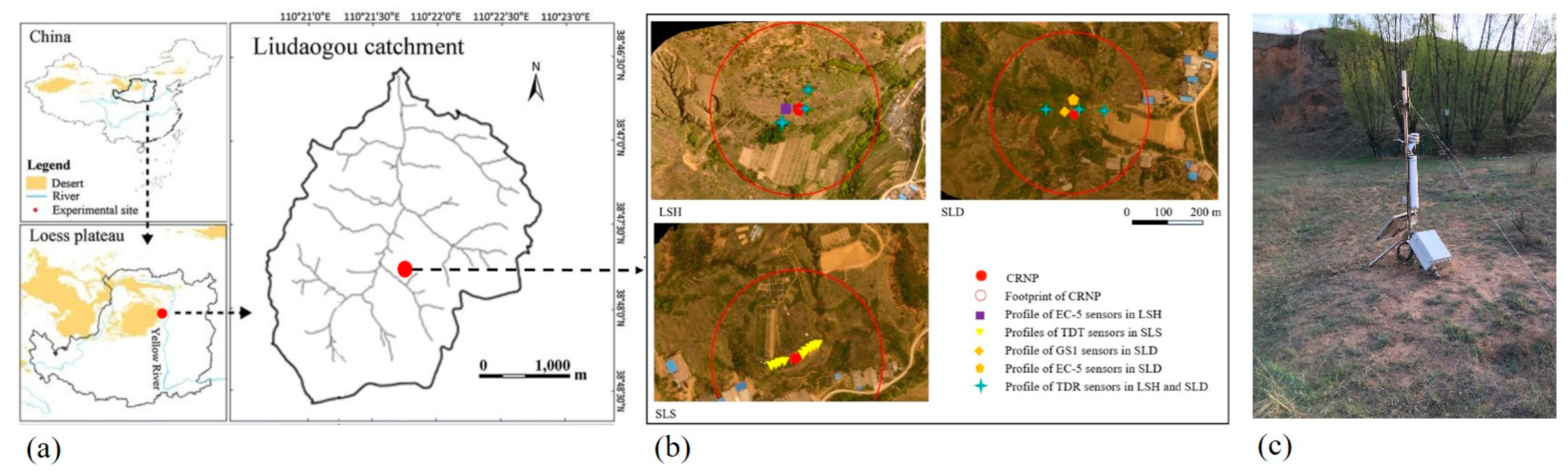
2.1. Site Description

This experiment was performed from 22 April to 15 October 2017 and from 15 April to 15 October 2018, carried out at the Erosion and Environmental Experiment Station, Northwest A&F University, in the Liudaogou Basin of the Loess Plateau (38.62° N, 110.35° E). The average elevation is 1181 m above sea level. The study region has a continental monsoon climate characterized by dry winters and wet summers, with a mean annual temperature of 8.4 °C and a mean annual precipitation of 437 mm. Approximately 80% of the total annual precipitation occurs in the rainy season, ranging from June to September [32]. The unique water–wind erosion interlaced region has been formed by the interaction between wind and water erosion in this area [33].

Three instrumented field plots were studied: a loamy sand hill plot (LSH), a silty loam dam plot (SLD), and a sandy loam slope plot (SLS), in one small watershed shown in Figure 1. The LSH plot has sand soil in shallow layers, but loessial and sandy soils are interlaced in the deep soil profiles, which were mainly formed via aeolian processes [34]. The LSH plot was mainly covered by grass, including Artemisia and Caragana korshinskii Kom, and approximately 70 poplar trees, and there is no farmland nor human disturbance. For soil and water conservation, dams were built across the water flow gully so that the sediment was deposited as dam lands in front of barriers. The SLD plot was set in a dam land with loessial soil. In the SLD plot, the sediments were primarily from the loss of the original soil, which consists mainly of loessial and sandy soils, and from the selectivity of detachment as well as transport processes [35]. Part of this plot is farmland planted with corn, and the rest was mainly covered with Artemisia and a few Populus simonii Carr as well as Salix matsudana Koidz. trees. The SLS plot is on a slope of 15° with the existence of eroded gullies, and the soil texture is loessial soil, which is formed through water and wind erosion of the loessial parental material [36]. There are some other experiments performed in the SLS. The SLS plot was mainly covered by grass, including Stipa bungeana, which was mostly distributed in the area where no experiment is being performed, Medicago sativa L., and a small amount of Glycine max (L.) Merr. The soil textures and terrains of the three plots are presented in

Table 1. Soil mechanical composition, soil texture, and terrain of the CRNP plots. The soil types were classified according to the international soil classification system.

	LSH	SLD	SLS
Bulk density (g cm−3)	1.56	1.35	1.34
Soil total porosity (%)	41.13	47.27	49.43
Sand content (2−0.02 mm, %)	84.20	15.73	51.91
Silt content (0.02–0.002 mm, %)	6.50	62.67	36.10
Clay content (<0.002 mm, %)	9.30	21.60	11.99
Organic matter content (g kg−1)	0.19	1.49	0.22
Saturated hydraulic conductivity (cm h−1)	35.45	9.86	22.21
Field capacity (cm3 cm−3)	0.11	0.33	0.28
Soil type	Loamy sand	Silty loam	Sandy loam
Terrain	Hilly	Check dam	Sloped

.

2.2. SWC Sensors

In LSH and SLD plots, one cosmic ray neutron probe (CRNP) (Probe Science and Technology Ltd., Beijing, China) and three profiles of time domain reflectometry (TDR) sensors (TDR310S, Acclima, Inc. Meridian, ID, USA) buried at different depths and covered by different vegetation were established, respectively (Figure 1). In the SLS plot, one CRNP and nine profiles of time domain transmissometry (TDT) sensors (Acclima, Inc. Meridian, ID, USA) buried at different depths and covered by different vegetation were established. CRNPs, TDR sensors, and TDT sensors are used to measure temporal SWCs on two scales and different depths of the three plots. The distribution of sensors and plant species in the plots are listed in

Table 2. Soil water content sensors installed in the three CRNP plots.

Plot	Sensor Type	Plant Species	Depth of Sensors (m)	Distance between Profile and CRNP (m)	Number of Profiles
LSH	TDR310S	Caragana korshinskii	0.10, 0.20, 0.50, 1, 2, and 4	0.5	1
	TDR310S	Artemisia	0.10, 0.20, 0.50, 1, 2, and 4	30	1
	TDR310S	Salix matsudana	0.10, 0.20, 0.50, 1, 2, and 4	30	1
SLD	TDR310S	Artemisia	0.10, 0.20, 0.50, 1, 2, and 4	0.5	1
	TDR310S	Caragana korshinskii	0.10, 0.20, 0.50, 1, 2, and 4	72	1
	TDR310S	Zea mays Linn.Sp.	0.10, 0.20, 0.50, 1, and 2	70	1
SLS	TDT	Medicago sativa	0.05, 0.15	7.5, 12.5, and 17.5	3
	TDT	Artemisia	0.05, 0.15	2.5, 2.5, and 7.5	3
	TDT	Glycine max	0.05, 0.15	12.5, 17.5, and 22.5	3

. All of the SWC sensors were calibrated through the oven-dried method, which obtained the SWC samples from profiles near the sensors and depths in the same manner.

2.3. The Spatial Distribution of SWC

The multipoint of SWC in 3 plots was manually measured via a time domain reflectometer, TK1502C (Tektronix 1502C, Tektronix, Inc., Beaverton, OR, USA), with a probe with a length of 30 cm. Measurements were taken using a grid-like pattern separated by 10 m and sticking the TK1502C probe into the ground to a depth of 30 cm 11 times (17 April, 28 May, 9 and 20 June, 5 and 24 July, 4 and 26 August, 4 and 27 September, and 24 of October 2018). TK1502C measures SWC by calculating the dielectric constant, ${\epsilon }_d$:

$${\epsilon }_d={((x_2-x_1)/(L_{sensor}\times V_p))}^2$$

(1)

where x₁ and x₂ are the first and second reflection peaks of the soil conductivity waveform, respectively (m). $L_{sensor}$ is the length of the probe (m) and V_p is the velocity of propagation controls, read from the TK1502C probe.

The volumetric soil water content θ (cm³ cm⁻³) can then be calculated [37]:

$$\theta =-0.053+0.0292\times {\epsilon }_d-0.00055\times {\epsilon }_d{}^2+0.0000043\times {\epsilon }_d{}^3$$

(2)

Kriging interpolation calculated by ArcGIS was used to spatially map the weighted average SWC obtained by the TDR.

2.4. The CRNPs

There is one CRNP installed at the center of each plot. Every CRNP consists of one CRP100 neutron sensor and a corresponding circuit, connecting to one data acquisition system with a solar power supply. A Vaisala HMP50 RHT sensor and tipping bucket rain gauge were installed to measure air pressure and temperature, humidity, and precipitation for calibrating the CRNPs. The accurate positions of the CRNPs were N38.79698, E110.35963 in the LSH, N38.79457, E110.36480 in the SLD, and N38.79455, E110.36172 for the SLS. The CRNP data were collected from 15 April to 15 October 2017 and from 15 April to 15 October 2018, with a time interval of 1 h.

2.4.1. Horizontal and Vertical Footprints of the CRNPs

The sensing radius of the CRNPs, R, defined as 86% of the cumulative sensitivity at sea level (air pressure of 1013 hPa) [15], is 130 m < R < 240 m [17]:

$$f_p=\frac{0.5}{0.86-e^{-P/P_0}}\approx P_0/P$$

(3)

where $f_p$ is the air pressure influence factor, P is the air pressure in the study area, and P₀ is the standard air pressure (1013hPa).

The vegetation influence factor, $f_{veg}(\theta )$, is calculated as follows [17]:

$$f_{veg}(\theta )=1-0.17(1-e^{-0.41H_{veg}})(1+e^{-7\theta })$$

(4)

where θ is SWC (m³ m⁻³) and H_veg is the height of the vegetation (m).

$$R(h,\theta ,p,veg)=f_p\times f_{veg}(\theta )\times R(h,\theta )$$

(5)

where $R(h,\theta ,p,veg)$ is the final radius and $R(h,\theta )$ is the radius without calibration of air pressure and vegetation.

The detecting depth of the CRNPs, D (cm), is defined as the depth at which 86% of the neutrons are detected. The measuring depth decreases as SWC increases [16]. The improved calculation equation [17] is as follows:

$$D={\rho }_{bd}{}^{-1}\left(p_0+p_1\left(p_2+e^{-r/100}\right)\frac{p_3+\theta }{p_4+\theta }\right)$$

(6)

where ${\rho }_{bd}$ is the soil bulk density (g cm⁻³). Numerical parameters are provided in Table A1 of Köhli et al. [17], where p_i is an empirical constant, p₀ = 8.321, p₁ = 0.14249, p₂ = 0.86655, p₃ = 26.42, and p₄ = 0.0567.

The footprint radius ranges from 130 to 240 m depending on air humidity, soil moisture, and vegetation [17]. In the study area, the horizontal footprints of the CRNPs in the three plots ranged from 148 to 174 m, 127 to 170 m, and 126 to 174 m for LSH, SLD and SLS, respectively, and the maximum measuring depths of the CRNPs were 59.8, 25.9, and 45.1 cm for LSH, SLD, and SLS, respectively [4].

2.4.2. Calibration of Neutron Intensity and the CRNPs

Neutron intensity is influenced by air pressure, humidity, and solar activity, therefore requiring calibration. Desilets et al. [11] corrected the effect of air pressure with latitude and altitude by using the following equation:

$$N_p=N_{raw}\exp \left[\left(P_0-P\right)/L_a\right]$$

(7)

where $N_{raw}$ is the raw value of the neutron intensity detected by the CRNPs, P₀ is the standard air pressure (1013hPa), and $L_a$ is the mass attenuation length for high-energy neutrons (g cm⁻²), varying from 128 g cm⁻² at high latitudes to 142 g cm⁻² near the equator [6]. A value of 136 g cm⁻² for $L_a$ in this study area was used [4].

The correction of air humidity [12] is calculated as follows:

$$N_{pw}=N_p(1+0.0054(\rho -{\rho }_0))$$

(8)

where $N_{pw}$ is the neutron density per hour calibrated by air humidity and air pressure, $\rho$ is the absolute vapor density (g m⁻³) at a CRNP site, and ${\rho }_0$ is the reference vapor density (generally is 0 g m⁻³).

The intensity correction factor of solar activity, f_i [6], was used to correct the neutron count, where f_t is the measured neutron monitor intensity, yielding the final neutron count equation, written as follows:

$$N=\frac{N_{p\mathrm{w}}}{f_i}=N_{p\mathrm{w}}\times \frac{N_a}{N_m}$$

(9)

where N is the final neutron count, N_m is measured incoming neutron intensity at a given time, and N_a is the average neutron intensity during the period of measurement. The measured neutron flux data of N_m and N_a are from Jungfraujoch, Switzerland (http://cosray.unibe.ch/).

The corrected neutron flux has a negative and nonlinear relation with SWC. The N₀ method calculating function reported by Desilets et al. [9] is widely used to determine θ_CRNP (cm³ cm⁻³):

$${\theta }_{CRNP}=(\frac{a_0}{N/N_0-a_1}-a_2)\times {\rho }_{bd}$$

(10)

where N is the corrected neutron flux, N₀ is the neutron flux in the same condition but the soil is dry (obtained from the measured SWC in the footprint), and the parameters are a₀ = 0.0808, a₁ = 0.372, and a₂ = 0.115 [9]. θ_CRNP is SWC measured by the CRNPs (cm³ cm⁻³). It must be noted that the θ_CRNP calculated from Equation (10) is the total water content of a footprint that contains hydrogen, including soil water, soil lattice water, soil organic matter, and vegetation [6]. In Equation (10), soil bulk density is also needed to convert gravimetric SWC into volumetric SWC, because neutron counts are primarily converted into gravimetric water content via the N₀ method.

2.4.3. Calibration Soil Sampling

Calibrating sampling points were set every 60° around the CRNPs, at distances of 25 and 75 m from the CRNPs. Disturbed soil samples were collected at depths of every 5 cm to 30 cm at each point to obtain gravimetric SWC via the oven-dried method on 27 June, 23 July, 5 October 2016, and 6 May 2017. Undisturbed soil cores (100 cm³) were collected at each point by excavating 3 soil layers and sampling at depths every 10 cm to 30 cm to obtain the bulk density on 27 June 2016, therefore the volumetric SWC of 72 samples at each time were used to calculate N₀, which was reported in the previous study [4]. As recommended by Köhli et al. [17], 72 disturbed samples were collected from each plot during each sampling event; let θ_ij be a sample of soil moisture at the depth d_j and distance r_i to the CRNPs. The SWCs measured by the oven-dried method were weight averaged for calculating N₀ as follows:

(1) Vertical direction:

$$W_d\left(r,\theta \right)=e^{-2d/D}$$

(11)

where r is the distance between the sampling point and the CRNP, d is the depth of soil sample, and D is the measuring depth of the CRNP at the date of sampling.

(2) Horizontal direction:

$$W_r(h,\theta )\approx \left\{\begin{array}{l}{F}_1{e}^{-F_{2}r}+F_3{e}^{-F_{4}r},0.5m<r\le 50m\\ F_5{e}^{-F_{6}r}+F_7{e}^{-F_{8}r},50m<r\le 600m\end{array}\right\}$$

(12)

where F_i is individually dependent on humidity and SWC, but the W_r could be calculated by the application-ready scripts offered by Köhli et al. (2015) [17], which are also in the supporting information.

(3) The final weight-averaged SWC, <θ>, was then used to calculate N₀:

$$\langle {\theta }_k\rangle =\frac{{\displaystyle \sum _k{\theta }_k{W}_k}}{{\displaystyle \sum _k{W}_k}}$$

(13)

The equal weight, $W_{ij}=1\forall i,j$, was used to calculate the average field mean soil moisture <θ_ij> and field mean humidity <h>. It is recommended to calculate the weight in the vertical direction first and follow with the horizontal direction using Equations (11) and (12).

2.4.4. Vegetation Correction

The water in a vegetation canopy increases the density of hydrogen atoms near the surface, so the moderated fast neutrons are increased, reducing the density of fast neutrons detected by CRNPs, which would overestimate SWC and reduce the accuracy of CRNPs. Therefore, vegetation reduced the accuracy of CRNPs, so studies have proposed methods to improve the accuracy of SWC determination via CRNPs affected by vegetation. In this study, three vegetation calibration methods were used and evaluated, namely (1) the N₀(BWE) correction method (Veg–N₀); (2) the N/N₀ ratio method (Veg–N/N₀); and (3) the weighted SWC corrected method (Veg–WSWC).

(1) N₀ (BWE) corrected method (Veg–N₀): To account for the effects of above-ground vegetation varying with the season on the moderated neutron counts [7,26], Franz et al. [25] proposed the following correction factor to N₀:

$$N_0(BWE)=m\times BWE+N_0(0)$$

(14)

where $N_0(0)$ is the instrument-specific estimate of N₀ with no standing biomass, BWE is the biomass water equivalent (kg m⁻²), and m is the slope of the relationship between N₀ (BWE) and BWE, determined via in situ calibration datasets. The BWE is further defined as follows:

$$BWE=SWB-SDB+SDB\times f_{WE}$$

(15)

where SWB is the wet biomass per unit area (kg m⁻²), SDB is the dry biomass per unit area (kg m⁻²), and $f_{WE}$ = 0.494 is the stoichiometric ratio of H₂O to organic carbon (assuming that organic carbon is in the form of cellulose, C₆H₁₀O₅). Using nine field calibration datasets for maize and soybean crops, Franz et al. [25] found that there is a significant linear relationship between the N₀ and BWE of roving CRNPs, yielding N₀ (0) = 518.34 counts per minute and m = −4.9506 (R² = 0.515, P = 0.03), but Avery et al. [38] found that these coefficients are less suitable for forest canopies. The N₀ (BWE) in Equation (14) then replaces the N₀ in Equation (10) to estimate the SWC with vegetation correction.

(2) N/N₀ ratio method (Veg–N/N₀): The method proposed by Baatz et al. [13], using several temporary and permanent CRNPs within a network, is similar to that of Franz et al. [25], who found a linear correlation between the calibration parameter N₀ and dry above-ground biomass (AGB) or biomass water equivalent (BWE): a 0.9% reduction in fast-neutron intensity with increasing dry AGB (kg m⁻²) or 0.5% reduction in fast-neutron intensity with increasing BWE (kg m⁻²) was proposed. The vegetation correction yields as follows:

$$N_{0,B}(AGB)=-r_1\times AG{B}_{dry}+N_{0,B,AGB=0}$$

(16)

$$N_{0,B}(BWE)=-r_2\times BWE+N_{0,B,BWE=0}$$

(17)

where r₁ is the neutron count per hour (cph) per kg of dry AGB per m², and r₂ is the cph per kg of BWE per m², representing the variations of N₀ with AGB, AGB_dry (kg m⁻²), or BWE, BWE (kg m⁻²); $N_{0,B,AGB=0}$ and $N_{0,B,BWE=0}$ (cph) are the reference N₀ when AGB and BWE are 0 kg m⁻². From the ratio N/N₀ we then derive the more general relationship N/N₀ = N_e/N_0,B,AGB=0, where N_e is first corrected by an efficiency scaling factor [13], which is calculated as the ratio of the neutron intensity of one permanent CRNP and several temporary CRNPs, and then corrected by the vegetation factor. In this study, N_e is the fast-neutron intensity corrected for vegetation (v). The new vegetation-corrected neutron intensity, N_e, is then determined with the vegetation-corrected factor, $f_{veg-N/N_0}$; the vegetation correction factor can be obtained as follows:

$$N_e=N\times f_{veg-N/N_0}=\frac{N}{1-r_1/N_{0,B,AGB=0}\times AG{B}_{dry}}$$

(18)

$$N_e=N\times f_{veg-N/N_0}=\frac{N}{1-r_2/N_{0,B,BWE=0}\times BWE}$$

(19)

The implementation of the vegetation correction yields the relationship between the neutron intensity and total soil water content:

$$\theta =(\frac{a_0}{N_e/N_{0,B,AGB=0}-a_1}-a_2){\rho }_{bd}$$

(20)

(3) Weighted SWC corrected method (Veg–WSWC): Coopersmith et al. [26] corrected CRNP data with the LAI and took the spatial distribution of SWC into account:

$$SW{C}_v={\beta }_{1}SW{C}_c+{\beta }_2+{\epsilon }_e$$

(21)

where $SW{C}_v$ is the Kriging weighted average SWC measured via a TK1502C, which provides a simple mechanism for ascertaining the proportion of a given region closest to a defined set of points. The weight factor is the ratio of the area of a sensor’s Voronoi region and the total area of the domain for which an average soil moisture value is desired, being the footprint of a CRNP. $SW{C}_c$ is the CRNP SWC after the corrections of water vapor, air pressure, and solar activity. ${\beta }_1$ and ${\beta }_2$ are coefficients of linear regression. The residual (error), ${\epsilon }_e$ between the CRNP and Voronoi estimates, was modeled as a function of vegetation, using the LAI as a proxy measurement for the density of the vegetation present:

$${\epsilon }_e={\beta }_3\lambda +{\beta }_4$$

(22)

where ${\epsilon }_e$ is the residuals produced in Equation (21) and $\lambda$ denotes the measured LAI. Continuing, the measurements of the LAI themselves define an empirical relationship between the LAI and the day of the year.

Finally, by adjusting a CRNP estimate with LAI relationships, an approximate one-to-one relationship between these adjusted CRNP estimates and the Voronoi-based field averages from the in situ network was produced by combining Equations (21) and (22):

$$SW{C}_v={\beta }_{1}SW{C}_c+{\beta }_3\lambda (d)+{\beta }_5$$

(23)

In this case, $\lambda (d)$ is the estimate of the LAI on the day in the equation, ${\beta }_5={\beta }_2+{\beta }_4$.

2.5. Biomass Measurement

The 4–pro UAV (DJI–Innovations Inc., Guangdong Province, China) with a build-in visible-light camera was used to capture imageries to measure areas of each vegetation types of 3 plots. The RedEdge multispectral camera (MicaSence Inc., Seattle, USA) was used to estimate biomass, vegetation water content, and their spatial distribution [39,40,41,42]. The UAV flight height and image overlap were set to 140 m and 85%, respectively, to ensure the same resolution for three plots for both visible and RedEdge multispectral images. Pix4Dmapper software (Pix4D S.A. EPFL Inc., Lausanne, Switzerland) was employed to stitch images automatically, perform geometric correction, and apply Gaussian mean filtering. The stitched visible images were used to distinguish between different vegetation types and to estimate their growth areas as well as distances to the CRNPs based on the color and pixel location. The stitched RedEdge multispectral images facilitated the estimation of the vegetation water content and biomass quantity. Because the ratio vegetation index (RVI) is sensitive to green vegetation [43], and the remote sensing images were obtained at the peak of vegetation growth, on 30 June 2018, the RVI was selected for the inversion of biomass in this study. ENVI software (Harris Geospatial Solutions. Inc., Broomfield, USA) was used to extract the RVI.

According to vegetation type and distribution, samples representing typical vegetation and density were selected to be sampled. Biomass samples were harvested in 1 × 1 m plots, and the GPS sample data were recorded and used to locate the sampling points in the imageries to estimate the spatial biomass distribution for comparison to estimate the RVI. The aboveground vegetation harvested was weighed to obtain the fresh weight, after which samples were dried for 30 min at 105 °C and then 30 h at 75 °C in the laboratory. The dry AGB and vegetation water content obtained were then used for the calibration of the RVI data. The correlation between biomass and the RVI was analyzed, with the RVI as the independent variable and biomass as a dependent variable. The cubic polynomial functions were selected after a univariate regression analysis. The same procedure was applied to the vegetation water content and RVI relationships for calibration on 30 June 2018. The UAV measurement was carried out on 30 June 2018, but vegetation sampling procedures were followed monthly during the experiment so that the variation in biomass could be estimated according to the samples and distances to the CRNPs of each different vegetation type.

To obtain the horizontal weighting for these samples, a polynomial function was used [2] to describe the relationship between the cumulative fraction of counts (CFoC) and CRNP footprint radius (r), with the resulting horizontal weights shown in

Table 3. Cumulative fraction of counts (CFoC) values for four different radii (50 m segments) and horizontal weights (w_h).

r (m)	CFoC	Segment	wh
50	0.298	0–50	0.431
100	0.471	50–100	0.250
150	0.594	100–150	0.178
200	0.692	150–200	0.142

.

The cubic polynomial model between the reflectance index and above-ground biomass wet weight and vegetation water with the highest R² was selected to estimate biomass and vegetation water. The models are written as follows:

y = 3.1946x³ − 58.02x² + 317.03x − 195.44

(24)

y = 4.9127x³ − 79.849x² + 391.82x − 248.09

(25)

where x is the measured reflectance index and y is the above-ground biomass wet weight in Equation (24) (R² = 0.70) as well as the vegetation water (kg) in Equation (25) (R² = 0.71).

3. Results

3.1. The Calculation of the N₀ and Footprint of a CRNP

Considerable temporal variability is exhibited by N₀ when calibrated at different times, as seen in

Table 4. N₀s and RMSEs in each sampling date are between the CRNP SWCs estimated from N₀ at that sampling date and oven-dried SWCs at the other 3 sampling dates.

Date	N0			RMSE (cm3 cm−3)
	LSH	SLD	SLS	LSH	SLD	SLS	Total
27 June 2016	5109	6176	4930	0.099	0.151	0.102	0.120
23 July 2016	4677	6295	4316	0.051	0.030	0.100	0.068
5 October 2016	3763	5254	4246	0.119	0.171	0.080	0.121
6 May 2017	4547	5179	5323	0.088	0.09	0.106	0.099

, where the RMSE for each sampling date is between CRNP SWCs estimated from N₀ at that sampling date and the oven-dried SWCs in the other three sampling dates. It shows that N₀ changed sharply from June and July to October when the biomass was changing. The SWCs estimated by the CRNPs are directly affected by which soil sampling campaign is adopted for calibration. Table 4 also shows that the RMSE for each sampling date is between the CRNP SWCs estimated from N₀ at that sampling date and the oven-dried SWCs at the other three sampling dates. The RMSE of sampling on 23 July 2016 was the lowest, so the N₀ of soil sampling on this date was used to calculate the SWC.

The R ranged from 134 to 168 m, 120 to 177 m, and 134 to 181 m for LSH, SLD, and SLS, respectively. The D ranged from 18 to 61 cm, 10 to 29 cm, and 12 to 43 cm for LSH, SLD, and SLS, respectively.

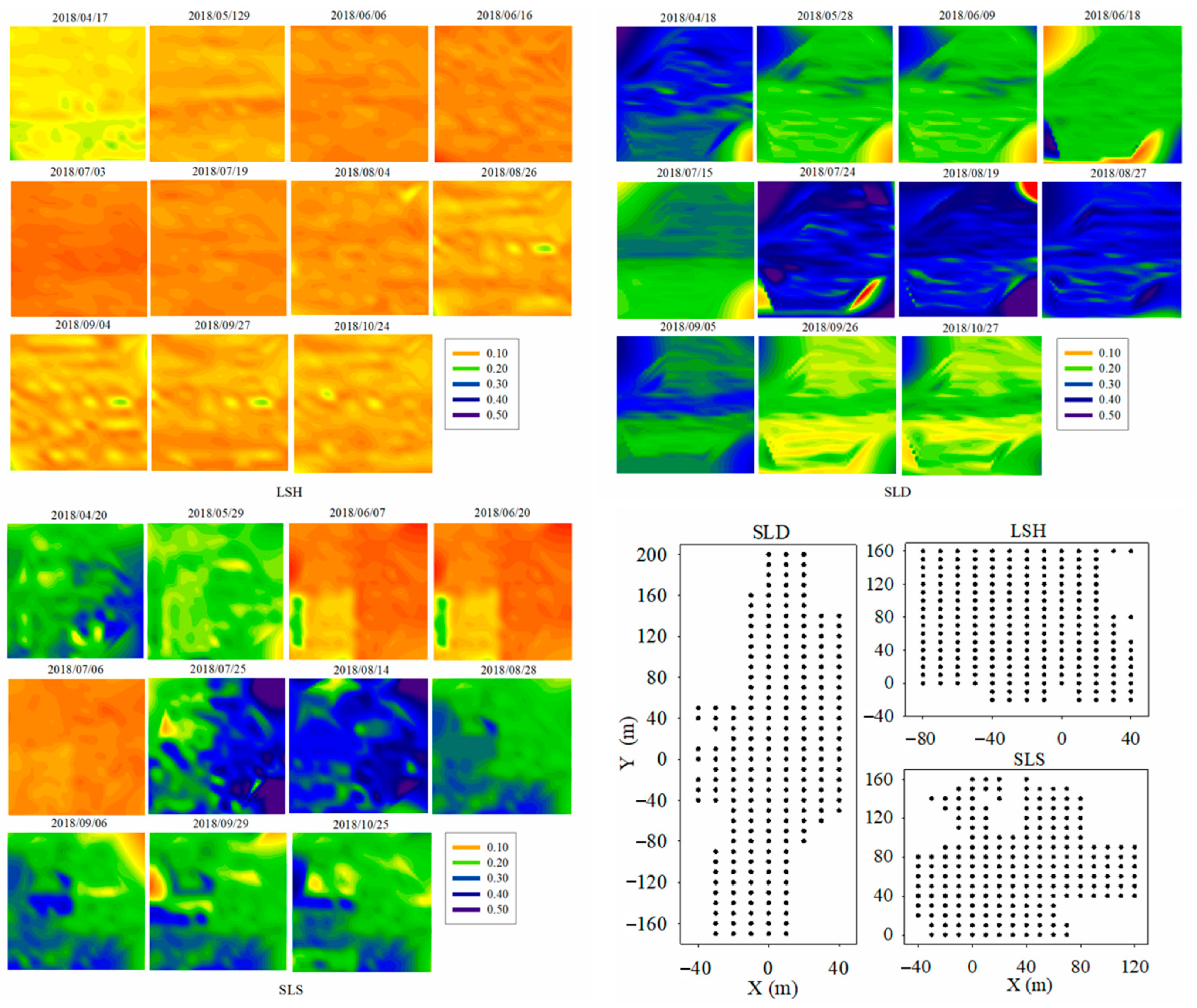
3.2. The Spatial Distribution of SWC

The temporal variations in the spatial distribution of SWC in the three plots are shown in Figure 2. The SWC values were low before July but increased distinctively during July and August due to rainfall, then subsequently decreased after September in SLD and SLS. In LSH, the SWC was lower and more stable than that in SLD and SLS. The uneven spatial distribution of the SWC lead to an uneven spatial distribution in vegetation, which reduced the spatial representation of the measured SWC and made it difficult to calibrate the effect of vegetation on the CRNPs.

The daily average CRNP SWCs were consistent with the Kriging-weighted average SWCs shown in Figure 3, except that the CRNP SWC was much higher than the weighted SWC on the 24 July in SLD. The CRNP SWC estimated from the N₀ of soil sampling on 23 July 2016 without vegetation calibration was higher than the Kriging-weighted SWC in SLD and lower than the Kriging-weighted SWC in LSH and SLS, possibly because SLD had higher biomass than LSH and SLS, besides, the different sampling dates between the calibration and vegetation sampling also resulted in the differences between the CRNP SWC and Kriging-weighted average SWC. The SWC estimated from the CRNPs showed significant correlations with the weighted average SWC (p < 0.01), with the corresponding R² values of LSH (0.79) > SLS (0.62) > SLD (0.52).

3.3. The Effects of Vegetation on CRNPs

The hydrogen consistency of vegetation, which the hydrogen of vegetation water adds to the CRNP signal, overestimating the SWC in SLD and underestimating the SWC in LSH and SLS, thus requires vegetation calibration. The vegetation biomass was spatially quantified relative to the CRNPs using the UAV and RedEdge multispectral camera in order to account for the biomass effects that decrease with distance from the CRNPs. Due to the presence of erosion gullies, the terrain is broken and uneven in the footprints of the CRNPs, resulting in the areas of four radii varying, and they are shown in

Table 5. The dry above-ground biomass and vegetation water in total and four radial segments of the three plots estimated from the multispectral camera on 30 June 2018.

Plot	Radial Segment (m)	0–50	50–100	100–150	150–200	Total
LSH	Area (m2)	7850	23,550	39,250	41,213	111,863
	Above-ground biomass (kg m–2)	0.30	0.38	0.40	0.33	0.36
	Vegetation water (kg m–2)	0.32	0.40	0.43	0.36	0.39
SLD	Area (m2)	7850	11,775	9812	13,737	43,175
	Above-ground biomass (kg m–2)	0.54	0.44	0.58	0.32	0.45
	Vegetation water (kg m–2)	0.59	0.47	0.55	0.30	0.46
	Area (m2)	7137	17,663	14,719	13,738	53,969
SLS	Above-ground biomass (kg m–2)	0.40	0.39	0.53	0.39	0.43
	Vegetation water (kg m–2)	0.43	0.41	0.52	0.41	0.44

.

The distributions of biomass and vegetation water of four radii measured on 30 June 2018 are shown in Figure 4 and Figure 5. The total dry above-ground biomass and vegetation water quantity in each of the three plots are presented in Table 5. Additionally, the changes in measured and simulated total dry AGB (kg) and vegetation water per m² (kg m^–2) of the three plots are shown in Figure 6.

The CRNP SWCs of the three plots were calibrated, and Figure 7 shows the CRNP SWCs in 2018 corrected by three different methods. The Veg–N₀ method yielded similar trends at the LSH and SLD sites, which was lower than CRNP SWC without vegetation calibration when biomass was low and higher than it when biomass was high; however, in SLS, the SWC calibrated via the Veg–N₀ method was always lower than the CRNP SWC without vegetation calibration. The SWC calibrated via the Veg–N/N₀ method was very close to the CRNP SWC without vegetation calibration among the three plots. The SWC calibrated via the Veg–WSWC method performed differently in SLS, estimating the highest SWC in SLS. At the LSH site, the CRNP SWC and SWCs calibrated by the three methods were below 0.2 cm³ cm⁻³, which is reasonable considering the soil texture in LSH. However, in SLD and SLS, the SWCs during the period of mid-July to August are unreasonably high, likely because during and after precipitation soil is saturated and runoff as well as ponded water on the surface are formed; these water did not infiltrate into soil to form soil moisture but increased the hydrogen density, which was observed by the CRNPs. This being the case, the CRNPs overestimated the SWC. For the SLD site, the SWC values calibrated by the three methods were lower than the SWC values without calibration. Although the calibration methods were performed differently, they exhibited similar patterns for each plot. As

Table 6. Soil water content RMSEs for the three different CRNP sites estimated using the three different vegetation calibration methods (Veg–N₀, Veg–N/N₀, and Veg–WSWC) and Kriging-weighted average SWCs estimated from a TK1502C in 2018.

Plots	RMSE without Vegetation Calibration (cm3 cm−3)	RMSE of Three Vegetation Calibrations without Horizontal Weighting (cm3 cm–3)			RMSE of Three Vegetation Calibrations with Horizontal Weighting (cm3 cm–3)
		Veg–N0	Veg–N/N0	Veg–WSWC	Veg–N0	Veg–N/N0	Veg–WSWC
LSH	0.053	0.022	0.030	0.034	0.020	0.024	0.028
SLD	0.100	0.068	0.078	0.082	0.062	0.072	0.078
SLS	0.127	0.032	0.052	0.041	0.011	0.035	0.032

shows, all three methods reduced the RMSE between the CRNP SWC and the Kriging-weighted SWC, indicating that vegetation calibrations improve the accuracy of the CRNP estimation of the SWC, with the Veg–N₀ method having the best estimation. The LSH revealed the lowest RMSE in both conditions with and without calibration, because the biomass at LSH was the lowest value due to a coarser soil texture than the other plots. The soil texture in LSH is loamy sand, with the highest saturated hydraulic conductivity and the lowest organic matter content of the plots, so the SWC is always low, resulting in the low biomass.

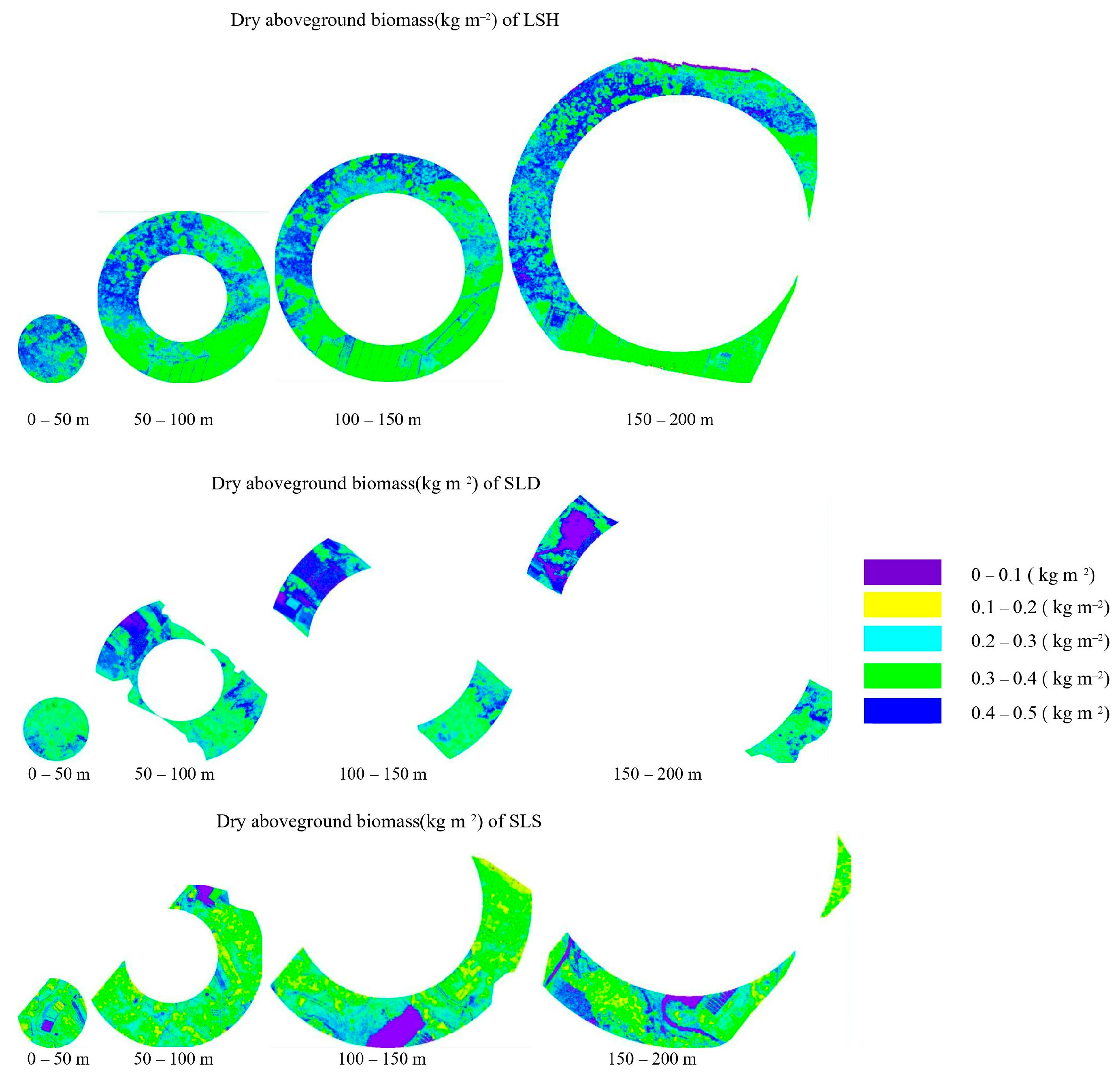
3.4. The Effects of the Spatial Distribution of Vegetation on CRNPs

Because the distribution of vegetation is typically heterogeneous within the experimental site of the Loess Plateau, applying simple modeling approaches is less effective. To address the complexities of biomass distribution and vegetation water content, a UAV was used to image the areas and distances of different vegetation types using a multispectral camera. The recorded above-ground biomass and vegetation water contents per m² of four radial segments are presented in Table 5. The weighted biomass of three sites was calculated and used to correct the vegetation spatial distribution calibrations. Table 6 shows the results of the three vegetation calibration methods with decreasing RMSEs using the spatial distribution correction, indicating that the calibration of vegetation distribution can further improve the accuracy of the CRNP estimates of the SWC. The Veg–N₀ method decreased RMSEs the most, followed by the Veg–WSWC method in LSH and SLD and by the Veg–N/N₀ method in SLS, indicating that the Veg–N₀ method was the most effective calibration for the CRNP vegetation of the three sites in the Loess Plateau. After applying the horizontal weighting of vegetation, the RMSEs of three vegetation calibrations were decreased, indicating that the calibration of the spatial distribution of vegetation is necessary and improves the accuracy of CRNP estimates of the SWC. If we assume uniform vegetation distribution and there is an equal impact of vegetation on CRNPs, the CRNPs would underestimate the SWC, and the higher the biomass content the larger the error estimate. Considering the non-uniform landscape, vegetation, and SWC of the undulating surface of the Loess Plateau, the vegetation distribution calibration improved the estimation of the SWC via the use of CRNPs. This study, therefore, has the potential to enhance CRNP applications, especially in footprints where species and biomass differ greatly. The additional challenges of how to evaluate the weighting factors need further research, including the additional calibration of below-ground biomass. The RMSEs of SWC estimation at the three sites were minimized for scenarios with—and without—spatial calibration considerations according to LSH < SLS < SLD.

4. Discussion

4.1. Calculating and Selecting N₀

The N₀ method was first proposed to estimate the SWC from neutron flux [9] and was used to verify the accuracy [4,21,41]. Table 4 shows that the RMSE in this study is poorer than that observed in prior studies [21,41], which may be because the heterogeneity spatial distributions of the SWC and vegetation reduce the spatial representativeness of CRNPs to the SWC and the accuracy of CRNPs. The N₀ showed a weak correlation with plant height and the LAI [14,44], and a strong correlation with AGB [10]; therefore, correction of N₀ based on AGB measurements during the crop growth stages was suggested [26]. Baatz et al. [13] proposed that fast-neutron intensity decreases by 0.9% when dry AGB (kg m⁻²) increases or decreases by 0.5% when BWE (kg m⁻²) increases, which provides a quick vegetation correction of CRNP measurements. In this study, the same method, Veg–N/N₀, did not produce the same result, although it reduced the RMSE for the three plots. The different outcomes may be because the CRNPs were not corrected through the SWC efficiency-scaling factor. The water in vegetation canopies added hydrogen atoms and reduced the accuracy of the CRNPs, so the CRNPs overestimated the SWC in summer, but the N₀ could be selected according to the lowest RMSE from samples obtained when the biomass was best representing the average growing season conditions of the vegetation.

4.2. The Effects of the SWC Spatial Distribution on the CRNP Output

The spatial variation in the SWC affected the representation of CRNP-measured SWC. The variances and coefficient of variations (CVs) of the SWC measured via TDR within the three plots showed the order of LSH < SLD < SLS (

Table 7. The standard deviation and coefficient of variation of each TDR SWC measurement of the three plots.

Date	LSH		SLD		SLS
	SD	CV	SD	CV	SD	CV
17 April	0.013	0.086	0.033	0.105	0.036	0.142
28 May	0.011	0.105	0.021	0.091	0.021	0.099
9 June	0.008	0.089	0.010	0.127	0.038	0.407
20 June	0.008	0.090	0.010	0.127	0.038	0.408
5 July	0.008	0.116	0.028	0.217	0.010	0.122
24 July	0.018	0.116	0.050	0.131	0.064	0.202
4 August	0.014	0.148	0.046	0.125	0.053	0.160
26 August	0.018	0.164	0.025	0.076	0.031	0.120
4 September	0.021	0.189	0.150	0.571	0.096	0.420
27 September	0.018	0.164	0.035	0.186	0.031	0.120
24 October	0.018	0.164	0.027	0.081	0.096	0.420

), indicating that the spatial distribution of the SWCs of the three plots is in this order and that the high heterogeneity of the SWC spatial distribution reduces the representativeness of the CRNPs. In SLD, the CRNP SWC was much higher than the weighted SWC on 24 July, due to ponded water within the SLD CRNP footprint because of the rainfall between 17 and 21 July. Omitting this measurement for SLD, the R² becomes 0.75, and the order shifts to LSH (0.79) > SLD (0.75) > SLS (0.62), keeping in line with the spatial variations in the SWCs shown in Figure 2. This order shows decreasing representativeness with increasing spatial variation in the SWC, which matches the order of variances and CVs of the SWC in three plots completely.

Considering the terrain and vegetation cover in the SLD plot, the variation in the spatial distribution of the SWC is mainly due to the difference in vegetation cover resulting from the limitation of the terrain. The SLD plot was once river valley; because of the check dam, the surface of the center of the SLD plot is flatter than surroundings, so precipitation collected and crops are planted there, and the center of the SLD plot is the dominant area for the TDR measurements (TK1502C), as shown in Figure 2. The other area of the SLD plot is an erosion gully, formed with runoff and covered by grasses. However, in the SLS and LSH plots, the terrains are uneven and sloping with erosion gullies, so the distribution of these two plots are impacted by both terrain and vegetation cover. Coopersmith et al. [26] calibrated the CRNP SWC via the LAI and weighted SWC. Bogena et al. [21] proposed seven radial segments of footprints to weigh SWC horizontally to verify the CRNP estimate. Those studies obtained low RMSEs and confirmed the necessity of the spatial weighting of the SWC. Although the more accurate spatial weighting functions were proposed [17], the patchy distribution of vegetation complicates the calculations, so the simpler method is adopted in this study.

There is an interaction between the distribution of vegetation and the SWC, where the broken land surface results in an uneven distribution of soil texture and of the SWC on the Loess Plateau. This effect both influences the distribution of vegetation and creates greater water consumption where vegetation density is high, resulting in dry layers in deep soil [45]. Under these circumstances, the terrain and distribution of the SWC must be considered for environmental improvement and vegetation restoration efforts. The slope aspect, affecting the amount of solar radiation received, is more critical than the slope gradient and elevation in the SWC distribution at the hillslope domain. Thus, the SWC variations may differ under varying land-use types in different terrains during wet and dry periods. In addition, the SWCs in depressions across the landscape are generally higher than those on hillslopes during wet periods, but lower than those on the hillslope during dry periods [46]. In this study, where the CRNPs report a regional averaged SWC that does not reveal the distribution of the SWC, the hillslope may be lower than the CRNP SWC; in contrast, the SWCs in depressions may be higher than the reported CRNP SWCs during wet periods, and the opposite may be true during dry periods [46]. Additionally, the patterns of land use greatly affect the vertical distribution and quantities of soil water [47].

4.3. Effects of Vegetation on CRNPs

CRNPs are advantageous for automated and undisturbed determinations of SWC at large scales in varied ecosystems [39,40,41]. Among past studies, many proposed vegetation correction methods, which are linear functions between the calibration parameter N₀ and biomass [13,25] as well as plant height and the LAI [14], and linear relationships between the LAI and the error between the CRNP SWC and the weighted SWC [26]. The ratio of thermal and fast neutrons or that of fast and thermalized neutrons was used to correct for vegetation effects [27] or estimating biomass directly [28]. All vegetation calibration methods improved the accuracy of the CRNPs. In this study, the Veg–N₀ method with vegetation distribution achieved the lowest RMSE. Comparing the RMSEs of CRNP SWCs and weighted SWCs before and after the vegetation distribution correction, the RMSE was reduced by 18%, 24%, and 12% using the Veg–N/N₀, Veg–N₀, and Veg–WSWC methods, respectively. Considering that the RMSEs of Veg–N/N₀ were the highest, this method appears less useful for uneven terrain compared to the others. In this study, some erroneous negative values were produced when the biomass was minimal (e.g., in early April dry AGB was less than about 0.3 kg m⁻²), which is consistent with the results of Coopersmith et al. [26], whose low values of the LAI (0–1.7) corresponded with positive values of errors between CRNP SWCs and weighted average SWCs, and expected to improve the accuracy regardless of the source of error because it includes a regression of the CRNP data against the ground truth. The Veg–N₀ method achieved the lowest RMSE in this study. The Veg–N/N₀ method could be the simplest method if using the 0.9% reduction in fast-neutron intensity with increasing dry AGB (kg m⁻²) was proposed [13]. The original Veg–WSWC uses the LAI to calibrate CRNPs, which is easier to measure than biomass. Baroni et al. [14] proposed a limitation of the CRNP estimate of the SWC when the hydrogen sources (e.g., biomass) vary with seasons and the spatial distribution of the SWC is assessed, which suggests the need for the periodic re-evaluation of the spatial distribution of biomass and the SWC. The order of correlations between the CRNP SWC and Kriging-averaged SWC of the three plots was shown with R² values of LSH > SLS > SLD, and the biomass per m² of the three plots showed SLD > SLS > LSH. This indicates that vegetation water interferes with hydrogen density measured via CRNPs, leading to errors of CRNP SWCs and affecting the spatial average SWC estimated from CRNPs; erroneous negative values were produced when the biomass was low, and erroneous positive values were produced when the biomass was large. It should be noted that the biomass value in this study is lower than in many other studies [21,27]; low biomass and vegetation water may not have much impact on the CRNPs, but considering the limitation of water resources and low ecosystem carrying capacity, small changes in the SWC greatly influence the soil water availability under the condition of low soil moisture on the Loess Plateau. Therefore, the effects of low biomass and vegetation water content on the CRNPs should be calibrated accurately to ensure the formulation of water policies to maintain sustainable ecosystems on the Loess Plateau.

Secondary hydrogen pools, such as vegetation, affect not only the results of the CRNP SWCs but also the footprint of the CRNPs, and the sensitivity of CRNPs to hydrogen decreases with distance from the sensor [17]. This being the case, Köhli et al. [17] proposed distance-dependent weighting functions within the CRNP footprint to calculate the reducing effects of vegetation from CRNPs. This approach, however, is not suitable for heterogeneous plant canopies, such as on the Loess Plateau. An approach that can determine the biomass and vegetation distribution intuitively and easily is needed. The rapidly advancing UAV industry has a wide range of distance measurement and imaging methods with higher spatial resolution and accuracy compared to most satellite data. Such methods are used to determine the LAI [48], biomass, vegetation water quantity, and vegetation diversity [49]. UAVs were proven to be able to obtain the biomass of crops and grassland accurately with a high resolution on a large scale, indicating that the measurement and spatial distribution of biomass can be obtained accurately [50,51,52]. These UAV imaging methods are becoming more advanced and more abundant in their observation capabilities, which can efficiently and conveniently obtain more accurate ground observation data than the quadrat method over large spatial domains. On the Loess Plateau, UAVs can provide clear images showing vegetation types and distribution with a visible camera, in addition to being able to measure biomass and vegetation water content. Considering the limitation of broken surfaces on the Loess Plateau, a UAV is an optimal method to obtain accurate above-ground data, such as biomass, vegetation types, and spatial distributions. Going into this research, assuming that vegetation growth could be measured by a UAV more frequently, an accurate vegetation growth model could be established, leading to the vegetation calibration of CRNPs being simplified and improving the accuracy of CRNP estimates. Combining UAVs and CRNPs, researchers can measure the accurate biomass with a high temporal–spatial resolution, which could improve the precision of CRNP vegetation calibration, therefore providing SWC datasets with high temporal–spatial resolution on a large scale, especially in the uneven terrain. Therefore, CRNPs can even be used in uneven terrains and undisturbed non-uniform landscapes. Additionally, CRNPs could potentially be used to estimate areal biomass and snow cover [27,53,54]. Liu et al. [55] evaluated a CRNP in two different ecosystems and found that it is necessary to calibrate vegetation, especially in areas with high biomass variability.

The variation in vertical SWCs at the LSH and SLD sites is likely tied to the difference in vegetation distribution and rooting depth, where the SWC at SLD is greater than that at LSH. The high CV of the deeper SWC at SLD points to higher consumption of water, likely caused by denser and deeper-rooted plants at SLD. In semi-arid regions, vegetation water consumption should be considered in vegetation restoration and ecological construction with limited water. Although the sensing depth of the CRNP is about 10-60 cm on the Loess Plateau [4], it can provide a reference of SWC variation in root zones [20], which can reflect the variation in deep SWCs to a certain extent.

CRNPs have been widely used in various regions and ecosystems in the world because they monitor SWC on a hectometer scale automatically and nondestructively; for example, managing irrigation and water use efficiency in agro-ecosystems [56,57,58], hydrological research [59], and monitoring soil moisture in complex geomorphic and vegetative conditions [60]. CRNPs capturing fast neutrons accurately lay the foundation for a wide range of other applications; with the deepening of research, CRNPs have been widely used in monitoring vegetation biomass changes [14], winter snow monitoring [19] on a hectometer scale, and providing SWC data for hydrological modeling [61]. This study evaluated vegetation calibration methods and the correction of vegetation distribution, but the correction of vegetation distribution requires further research. Additionally, the soil density varies with depth [62], which may influence the footprint of CRNPs. Additionally, the accuracy of CRNPs could be influenced by rivers’ underground water.

5. Conclusions

Plant biomass adds to the hydrogen content of the near-surface environment, affecting CRNP estimates of SWCs. In this study, the N₀ calibration method for SWCs without vegetation calibration reduced the RMSE from 0.121 to 0.068. The vegetation calibrations implemented with the Veg–N₀ method reduced the RMSE to 0.022, 0.068, and 0.032 in the LSH, SLD, and SLS plots, respectively. The correction of vegetation calibrations with horizontal weighting implemented with the Veg–N₀ method further reduced the RMSE to 0.020, 0.062, and 0.011 in the LSH, SLD, and SLS plot, respectively. The RMSEs of all three sites were in the order of LSH < SLS < SLD for both with and without the calibration of vegetation spatial distribution. We found that, where the vegetation spatial distribution is not taken into account, the CRNPs can underestimate SWCs when the CRNP footprint is covered with non-uniform vegetation; the higher the biomass, the greater the error. Because the CRNPs detected neutrons reflected by the intercepted crop canopy moisture, while SWC sensors buried in the soil often did not, the CRNP SWC is overestimated compared to buried sensor responses, highlighting the need to monitor and account for the effects of biomass water content as well as use UAV imageries to measure the distribution of and variation in biomass accurately. The study makes up for the lack of vegetation calibration for CRNPs on the Loess Plateau and verifies an improved calibration approach for the consideration of SWCs and vegetation distribution within the CRNP footprint, which should help develop sustainable vegetation management strategies on the Loess Plateau.

References

1. Kodama, M.; Kudo, S. Response of atmospheric neutron fluxes to soil moisture content. Sci. Pap. Inst. Phys. Chem. Res. 1985, 79, 99–103. [Google Scholar]
2. Zreda, M.; Desilets, D.; Ferré, T.P.A.; Scott, R.L. Scott. Measuring soil moisture content non-invasively at intermediate spatial scale using cosmic-ray neutrons. Geophys. Res. Lett. 2008, 35, L21402. [Google Scholar] [CrossRef] [Green Version]
3. Andreasen, M.; Jensen, K.H.; Desilets, D.; Franz, T.E.; Zreda, M.; Bogena, H.R.; Looms, M. Status and perspectives on the cosmic-ray neutron method for soil moisture estimation and other environmental science applications. Vadose Zone J. 2017, 16, 1–11. [Google Scholar] [CrossRef] [Green Version]
4. Wang, Q.; Fan, J.; Wang, S.; Yong, C.; Ge, J.; You, W. Application and accuracy of cosmic-ray neutron probes in three soil textures on the Loess Plateau, China. J. Hydrol. 2018, 569, 449–461. [Google Scholar] [CrossRef]
5. Rosolem, R.; Hoar, T.; Arellano, A.; Anderson, J.L.; Shuttleworth, W.J.; Zeng, X.; Franz, T.E. Translating aboveground cosmic-ray neutron intensity to high frequency soil moisture profiles at sub-kilometer scale. Hydrol. Earth Syst. Sci. 2014, 18, 4363–4379. [Google Scholar] [CrossRef] [Green Version]
6. Zreda, M.; Shuttleworth, W.J.; Zeng, C.; Desilets, D.; Franz, T.; Rosolem, R. COSMOS: The COsmic-ray Soil Moisture Observing System. Hydrol. Earth Syst. Sci. 2012, 16, 4079–4099. [Google Scholar] [CrossRef] [Green Version]
7. Franz, T.E.; Zreda, M.; Rosolem, R.; Ferre, T. A universal calibration function for determination of soil moisture with cosmic-ray neutrons. Hydrol. Earth Syst. Sci. 2013, 17, 453–460. [Google Scholar] [CrossRef] [Green Version]
8. Shuttleworth, J.; Rosolem, R.; Zreda, M.; Franz, T. The COsmic-ray Soil Moisture Interaction Code (COSMIC) for use in data assimilation. Hydrol. Earth Syst. Sci. 2013, 10, 1097–1125. [Google Scholar] [CrossRef] [Green Version]
9. Desilets, D.; Zreda, M.; Ferre, T.P.A. Nature’s neutron probe: Land surface hydrology at an elusive scale with cosmic rays. Water Resour. Res. 2010, 46, W11505. [Google Scholar] [CrossRef] [Green Version]
10. Baatz, R.; Bogena, H.R.; Franssen, H.H.; Huisman, J.A.; Qu, W.; Montzka, C.; Vereecken, H. Calibration of a catchment scale cosmic-ray probe network: A comparison of three parameterization methods. J. Hydrol. 2014, 516, 231–244. [Google Scholar] [CrossRef]
11. Desilets, D.; Zreda, M. On scaling cosmogenic nuclide production rates for altitude and latitude using cosmic-ray measurements. Earth Planet. Sci. Lett. 2001, 193, 213–225. [Google Scholar] [CrossRef]
12. Rosolem, R.; Shuttleworth, W.J.; Zreda, M.; Franz, T.E.; Zeng, X.; Kurc, S.A. The effect of atmospheric water vapor on neutron count in the cosmic-ray soil moisture observing system. J. Hydrometeorol. 2013, 14, 1659–1671. [Google Scholar] [CrossRef] [Green Version]
13. Baatz, R.; Bogena, H.R.; Franssen, H.J.H.; Huisman, J.A.; Montzka, C.; Vereecken, H. An empirical vegetation correction for soil water content quantification using cosmic ray probes. Water Resour. Res. 2015, 51, 2030–2046. [Google Scholar] [CrossRef] [Green Version]
14. Baroni, G.; Oswald, S.E. A scaling approach for the assessment of biomass changes and rainfall interception using cosmic-ray neutron sensing. J. Hydrol. 2015, 525, 264–276. [Google Scholar] [CrossRef]
15. Desilets, D.; Zreda, M. Footprint diameter for a cosmic-ray soil moisture probe: Theory and monte carlo simulations. Water Resour. Res. 2013, 49, 3566–3575. [Google Scholar] [CrossRef]
16. Franz, T.E.; Zreda, M.; Ferre, T.P.A.; Rosolem, R.; Zweck, C.; Stillman, S.; Zeng, X.; Shuttleworth, W.J. Measurement depth of the cosmic ray soil moisture probe affected by hydrogen from various sources. Water Resour. Res. 2012, 48, W08515. [Google Scholar] [CrossRef] [Green Version]
17. Köhli, M.; Schrön, M.; Zreda, M.; Schmidt, U.; Dietrich, P.; Zacharias, S. Footprint characteristics revised for field-scale soil moisture monitoring with cosmic-ray neutrons. Water Resour. Res. 2015, 51, 5772–5790. [Google Scholar] [CrossRef] [Green Version]
18. Zhu, X.; Cao, R.; Shao, M.; Liang, Y. Footprint radius of a cosmic-ray neutron probe for measuring soil-water content and its spatiotemporal variability in an alpine meadow ecosystem. J. Hydrol. 2018, 558, 1–8. [Google Scholar] [CrossRef]
19. Schattan, P.; Baroni, G.; Oswald, S.E.; Schöber, J.; Fey, C.; Kormann, C.; Huttenlau, M.; Achleitner, S. Continuous monitoring of snowpack dynamics in alpine terrain by aboveground neutron sensing. Water Resour. Res. 2017, 53, 3615–3634. [Google Scholar] [CrossRef]
20. Peterson, A.M.; Helgason, W.D.; Ireson, A.M. Estimating field scale root zone soil moisture using the cosmic-ray neutron probe. Hydrol. Earth Syst. Sci. 2016, 20, 1373–1385. [Google Scholar] [CrossRef] [Green Version]
21. Bogena, H.R.; Huisman, J.A.; Baatz, R.; Franssen, H.J.H.; Vereecken, H. Accuracy of the cosmic-ray soil water content probe in humid forest ecosystems: The worst case scenario. Water Resour. Res. 2013, 49, 5778–5791. [Google Scholar] [CrossRef] [Green Version]
22. Villarreyes, R.C.A.; Baroni, G.; Oswald, S.E. Integral quantification of seasonal soil moisture changes in farmland by cosmic-ray neutrons. Hydrol. Earth Syst. Sci. 2011, 15, 3843–3859. [Google Scholar] [CrossRef] [Green Version]
23. Evans, J.G.; Ward, H.C.; Blake, J.R.; Hewitt, E.J.; Morrison, R.; Fry, M.; Ball, L.A.; Doughty, L.C.; Libre, J.W.; Hitt, O.E. Soil water content in southern england derived from a cosmic-ray soil moisture observing system—COSMOS-UK. Hydrol. Process. 2016, 30, 4987–4999. [Google Scholar] [CrossRef] [Green Version]
24. Hawdon, A.; Mcjannet, D.; Wallace, J. Calibration and correction procedures for cosmic-ray neutron soil moisture probes located across Australia. Water Resour. Res. 2014, 50, 5029–5043. [Google Scholar] [CrossRef]
25. Franz, T.E.; Wahbi, A.; Vreugdenhil, M.; Weltin, G.; Heng, L.; Oismueller, M.; Strauss, P.; Dercon, G.; Desilts, D. Using cosmic-ray neutron probes to monitor landscape scale soil water content in mixed land use agricultural systems. Appl. Environ. Soil Sci. 2016, 2016, 4323742. [Google Scholar] [CrossRef] [Green Version]
26. Coopersmith, E.J.; Cosh, M.H.; Daughtry, C. Field-scale moisture estimates using cosmos sensors: A validation study with temporary networks and leaf-area-indices. J. Hydrol. 2014, 519, 637–643. [Google Scholar] [CrossRef]
27. Tian, Z.; Li, Z.; Liu, G.; Li, B.; Ren, T. Soil water content determination with cosmic-ray neutron sensor: Correcting aboveground hydrogen effects with thermal/fast neutron ratio. J. Hydrol. 2016, 540, 923–933. [Google Scholar] [CrossRef]
28. Jakobi, J.; Huisman, J.A.; Vereecken, H.; Diekkrüger, B.; Bogena, H.R. Cosmic ray neutron sensing for simultaneous soil water content and biomass quantification in drought conditions. Water Resour. Res. 2018, 54, 7383–7402. [Google Scholar] [CrossRef] [Green Version]
29. Wu, Y.Z.; Huang, M.B.; Warrington, D.N. Black locust transpiration responses to soil water availability as affected by meteorological factors and soil texture. Pedosphere 2015, 25, 57–71. [Google Scholar] [CrossRef]
30. Shao, M.A.; Yang, W.Z.; Li, Y.S. Study on soil water availability in Loess region. J. Hydraul. Eng-Asce. 1987, 8, 40–46. (In Chinese) [Google Scholar]
31. Zhao, C.L.; Jia, X.X.; Zhu, Y.J.; Shao, M.A. Long-term temporal variations of soil water content under different vegetation types in the Loess Plateau, China. Catena 2017, 158, 55–62. [Google Scholar] [CrossRef]
32. Tang, K.; Hou, Q.; Wang, B.; Zhang, P. The environment background and administration way of Wind-Water Erosion Crisscross Region and Shenmu experimental area on the Loess Plateau. Mem. NISWC Acad. Sin. MWR 1993, 18, 2–15. (In Chinese) [Google Scholar]
33. Zhu, Y.; Shao, M. Spatial distribution of surface rock fragment on hill-slopes in a small catchment in wind-water erosion crisscross region of the Loess Plateau. Sci. China Ser. D Earth Sci. 2008, 51, 862–870. [Google Scholar] [CrossRef]
34. Li, Z.; Zhao, L.; Dou, S. Agrology; Chemical Industry Publishing House: Beijing, China, 2005; pp. 197–199. [Google Scholar]
35. Zhao, P.; Shao, M.; Zhuang, J. Fractal features of particle size redistributions of deposited soils on the dam farmlands. Soil Sci. 2009, 174, 403–407. [Google Scholar] [CrossRef]
36. Lin, C.G. Agrology; Agricultural Publishing House: Beijing, China, 1983; pp. 219–220. [Google Scholar]
37. Topp, G.C.; Davis, J.L.; Annan, A.P. Electromagnetic determination of soil water content: Measurements in coaxial transmission lines. Water Resour. Res. 1980, 16, 574–582. [Google Scholar] [CrossRef] [Green Version]
38. Avery, W.A.; Finkenbiner, C.; Franz, T.E.; Wang, T.; Nguy-Robertson, A.L.; Suyker, A.; Arkebauer, T.; Munoz-Arriola, F. Incorporation of globally available datasets into the roving cosmic-ray neutron probe method for estimating field-scale soil water content. Hydrol. Earth Syst. Sci. 2016, 20, 3859–3872. [Google Scholar] [CrossRef] [Green Version]
39. Heidbüchel, I.; Güntner, A.; Blume, T. Use of cosmic-ray neutron sensors for soil moisture monitoring in forests. Hydrol. Earth Syst. Sci. 2016, 20, 1269–1288. [Google Scholar] [CrossRef] [Green Version]
40. Han, X.; Rui, J.; Xin, L.; Wang, S. Soil moisture estimation using cosmic-ray soil moisture sensing at heterogeneous farmland. IEEE Geosci. Remote Sens. Lett. 2014, 11, 1659–1663. [Google Scholar]
41. Zhu, X.; Shao, M.; Jia, X.; Huang, L.; Zhu, J.; Zhang, Y. Application of temporal stability analysis in depth-scaling estimated soil water content by cosmic-ray neutron probe on the northern Tibetan Plateau. J. Hydrol. 2017, 546, 299–308. [Google Scholar] [CrossRef]
42. Zheng, H.; Cheng, T.; Zhou, M.; Li, D.; Yao, X.; Tian, Y.; Cao, W.; Zhu, Y. Improved estimation of rice aboveground biomass combining textural and spectral analysis of UAV imagery. Precis. Agric. 2018, 20, 611–629. [Google Scholar] [CrossRef]
43. Birth, G.S.; Mcvey, G.R. Measuring the color of growing turf with a reflectance spectrophotometer. Agron. J. 1968, 60, 640–643. [Google Scholar] [CrossRef]
44. Hornbuckle, B.; Irvin, S.; Franz, T.; Rosolem, R.; Zweck, C. The potential of the COSMOS network to be a source of new soil moisture information for SMOS and SMAP. In Proceedings of the 2012 IEEE International Geoscience and Remote Sensing Symposium, Munich, Germany, 22–27 July 2012; pp. 1243–1246. [Google Scholar]
45. Jiang, N.; Shao, M.A.; Wei, H.; Wang, Y.Q. Characteristics of water circulation and balance of typical vegetations at plot scale on the Loess Plateau of China. Environ. Earth Sci. 2013, 70, 157–166. [Google Scholar] [CrossRef]
46. Yu, B.; Liu, G.; Liu, Q.; Wang, X.; Feng, J.; Huang, C. Soil moisture variations at different topographic domains and land use types in the semi-arid Loess Plateau, China. Catena 2018, 165, 125–132. [Google Scholar] [CrossRef]
47. Wang, Y.; Shao, M.; Zhang, C.; Han, X.; Mao, T.; Jia, X. Choosing an optimal land-use pattern for restoring eco-environments in a semiarid region of the Chinese Loess Plateau. Ecol. Eng. 2015, 74, 213–222. [Google Scholar] [CrossRef]
48. Camille, L.; Philippe, B.; Guillaume, J.; Bruno, R.; Sylvain, L.; Baret, F. Assessment of unmanned aerial vehicles imagery for quantitative monitoring of wheat crop in small plots. Sensors 2008, 8, 3557–3585. [Google Scholar]
49. Boon, M.A.; Tesfamichael, S. Wetland vegetation integrity assessment with low altitude multispectral uav imagery. ISPRS Int. Arch. Photogramm. Remote Sens. Spat. Inf. Sci. 2017, 42, 55–62. [Google Scholar] [CrossRef] [Green Version]
50. Yue, J.; Yang, G.; Tian, Q.; Feng, H.; Xu, K.; Zhou, C. Estimate of winter-wheat above-ground biomass based on uav ultrahigh- ground-resolution image textures and vegetation indices. ISPRS J. Photogramm. 2019, 150, 226–244. [Google Scholar] [CrossRef]
51. Villoslada, M.; Bergamo, T.F.; Ward, R.D.; Joyce, C.B.; Sepp, K. A novel UAV-based approach for biomass prediction and grassland structure assessment in coastal meadows. Ecol. Indic. 2021, 122, 107227. [Google Scholar] [CrossRef]
52. Zhang, H.; Tang, Z.; Yang, B.; Meng, B.; Qin, Y.; Sun, Y.; Lv, Y.Y.; Zhang, J.G.; Yi, S.H. A non-destructive method for rapid acquisition of grassland aboveground biomass for satellite ground verification using UAV RGB images. Glob. Ecol. Conserv. 2022, 33, e01999. [Google Scholar] [CrossRef]
53. Franz, T.E.; Zreda, M.; Rosolem, R.; Hornbuckle, B.K.; Shuttleworth, W.J. Ecosystem-scale measurements of biomass water using cosmic ray neutrons. Geophys. Res. Lett. 2013, 40, 3929–3933. [Google Scholar] [CrossRef]
54. Kodama, M.; Nakai, K.; Kawasaki, S.; Wada, M. An application of cosmic-ray neutron measurements to the determination of the snow-water equivalent. J. Hydrol. 1979, 41, 85–92. [Google Scholar] [CrossRef]
55. Liu, C.; Jia, X.; Ren, L.; Zhu, X.; Shao, M. Evaluation of the soil water content of two managed ecosystems using cosmic-ray neutron sensing on China’s Loess Plateau. Eur. J. Soil Sci. 2023, 74, e13339. [Google Scholar] [CrossRef]
56. Brogi, C.; Pisinaras, V.; Koehli, M.; Dombrowski, O.; Franssen, H.; Babakos, K.; Chatzi, A. Monitoring Irrigation in Small Orchards with Cosmic-Ray Neutron Sensors. Sensors 2023, 23, 2378. [Google Scholar] [CrossRef]
57. Chen, X.; Song, W.; Shi, Y.; Liu, W.; Lu, Y.; Pang, Z.; Chen, X. Application of Cosmic-Ray Neutron Sensor Method to Calculate Field Water Use Efficiency. Water 2022, 14, 1518. [Google Scholar] [CrossRef]
58. Finkenbiner, C.E.; Franz, T.E.; Gibson, J.; Heeren, D.M.; Luck, J. Integration of hydrogeophysical datasets and empirical orthogonal functions for improved irrigation water management. Precis. Agric. 2019, 20, 78–100. [Google Scholar] [CrossRef] [Green Version]
59. Franz, T.E.; Wahbi, A.; Zhang, J.; Vreugdenhil, M.; Heng, L.; Dercon, G.; Strauss, P.; Brocca, L.; Wagner, W. Practical data products from cosmic-ray neutron sensing for hydrological applications. Front. Water 2020, 2, 9. [Google Scholar] [CrossRef] [Green Version]
60. Jeong, J.; Cho, S.; Lee, S.; Kim, K.; Lee, Y.; Lee, C.; Lee, S.; Choi, M. A Study on Domestic Applicability for the Korean Cosmic-Ray Soil Moisture Observing System. Korean J. Remote Sens. 2023, 39, 233–246. [Google Scholar]
61. Dimitrova-Petrova, K.; Geris, J.; Wilkinson, M.; Rosolem, R.; Verrot, L.; Lilly, A.; Soulsby, C. Opportunities and challenges in using catchment-scale storage estimates from cosmic ray neutron sensors for rainfall-runoff modelling. J. Hydrol. 2020, 586, 124878. [Google Scholar] [CrossRef]
62. Raghuram, A.; Mounika, N.; Basha, B.; Moghal, A. Soil Water Characteristic Curves of Soils Exhibiting Different Plasticity. Int. J. Geosynth. Ground Eng. 2023, 9, 25. [Google Scholar] [CrossRef]
Figure 1. Position of experiment station (a); overhead view of the three plots, namely loamy sand hill (LSH), silty loam dam (SLD), and sandy loam slope (SLS) (b); and CRNP (c).
Water 15 02766 g001
Figure 2. Temporal variations in the SWC spatial distributions and the sampling point distributions in each of the three plots.
Water 15 02766 g002
Figure 3. Daily average SWCs estimated from the CRNPs and 0–30 cm Kriging-weighted average SWCs in three plots on 17 April, 28 May, 6 and 16 June, 3 and 19 July, 4 and 26 August, 4 and 26 September, and 24 October 2018. The error bars are standard deviations.
Water 15 02766 g003
Figure 4. The dry above-ground biomass (kg m−2) in four radial segments of the three plots.
Water 15 02766 g004
Figure 5. The vegetation water contents (kg) in four radial segments of the three plots.
Water 15 02766 g005
Figure 6. The changes in the measured and simulated total dry AGB (kg) and vegetation water per m2 (kg m–2) of the three plots.
Water 15 02766 g006
Figure 7. The CRNP SWC values corrected via the Veg–N0, Veg–N/N0, and Veg–WSWC methods in the LSH, SLD, and SLS sites during 2018.
Water 15 02766 g007