Influences of the Runoff Partition Method on the Flexible Hybrid Runoff Generation Model for Flood Prediction

Abstract

The partition of surface runoff and infiltration is crucial in hydrologic modeling. To improve the flood prediction, we designed four strategies to explore the influences of the runoff partition method on the flexible hybrid runoff generation model. The runoff partition strategies consist of a hydrological model without the runoff partition module, a two-source runoff partition method, an improved two-source runoff partition method considering the heterogeneity of the subsurface topography and land cover, and a three-source runoff partition method. The Xin’anjiang hydrological model was used as the modeling framework to simulate a six-hourly stream flow for the Xun River watershed in Shaanxi Province, China. And the saturation-excess runoff generation and infiltration-excess runoff generation mechanisms were combined to construct the flexible hybrid runoff generation model. The performances of the four strategies were compared and analyzed based on the continuous flow discharge as well as the flood events. The runoff components analysis method was used to test the model’s conformity with the reality of the watershed. The results showed that the three-source runoff partition method was not applicable to the flexible hybrid runoff generation model because it overestimated the surface runoff and almost ignored the subsurface stormflow runoff. The improved two-source runoff partition method outperformed the others as it considered the heterogeneity of the watershed.

1. Introduction

A hybrid runoff generation process pattern comprised of multiple mechanisms can often happen in semi-arid, semi-humid, and mountainous watersheds due to the heterogeneity of meteorological factors and underlying surface conditions (i.e., rainfall, land covers, soil types, etc.) [1,2,3,4]. Runoff generated by the integration of the three components, including the subsurface stormflow runoff, saturation-excess runoff, and infiltration-excess runoff generation, is known as hybrid runoff, which leads to rapid flood occurrences and high flood peak discharges, and thus makes hydrological forecast even more challenging [5,6].

Hydrological modeling using conceptualized hybrid runoff generation mechanisms attracted lots of attention to solve the limitations of single runoff generation mechanisms [7]. Lots of conceptual mixed runoff generation models have been developed, for instance, the vertically mixed runoff generation model [8], the XAJ–Green–Ampt model [7], as well as the variable infiltration capacity (VIC) runoff generation model [9], and so on. These hybrid runoff generation models were constructed in accordance with the vertical combination of saturation-excess and infiltration-excess modules or in accordance with the spatial combination of saturation-excess and infiltration-excess modules [2]. The current mixed runoff generation models can acquire a good performance in the semi-humid and semi-arid regions but also have some shortcomings. For instance, they assumed that a fixed runoff generation mechanism dominated each natural watershed. This assumption could not reflect the heterogeneity of the dominant runoff generation mechanisms within a basin [5,10,11]. To this end, the study of hydrological modeling has recently progressed toward developing and applying flexible models, which provided a new method for solving flood forecasting issues in semi-arid, semi-humid, and mountainous areas [5].

The flexible hydrological modeling framework allowed for the selection of alternative representations of runoff processes and various combinations of both linear and nonlinear components [12]. This kind of model can be regulated timely to construct a suitable model structure for a particular basin [5]. A lot of research has been carried out recently on developing flexible framework models. For example, Liu et al. [5] developed a novel flexible hybrid runoff generation modeling framework appropriate for hydrological modeling in semi-arid and semi-humid areas, which is known as the spatial combination computing models for runoff generation (SCCMs). Huang et al. [12] discussed the performances of four traditional hydrological models and compared them with those of four flexible models for semi-arid environments. Yi et al. [2] proposed an improved flexible hybrid runoff generation strategy and compared its accuracy with that of four traditional flexible strategies. The fundamentals of the flexible hybrid runoff generation models discussed above were the combinations of three single runoff generation mechanisms, sometimes one or two.

In the land surface hydrological processes, different water balance components are closely related and interact with each other. An inappropriate separation of runoff components directly or indirectly influences the simulations of other water balance components [13]. Runoff partition methods can also be significant for flexible runoff generation modeling [14]. While runoff generation dominates the simulated discharge volumes, runoff separation dominates the simulated hydrograph shapes. It is generally accepted that the hydrograph is comprised of different components with various response times, such as a fast or a slow runoff component [15,16,17,18]. The fast runoff may further be separated into surface flow and subsurface stormflow, and the slow runoff represents subsurface flow [19,20]. In addition, the same runoff component may originate from different runoff generation mechanisms [2,21]. For instance, surface runoff may originate from saturation excess or infiltration excess [22]. This issue can also be studied by using the runoff partition methods.

Several runoff partition methods have been commonly adopted in previous studies. The XAJ model proposed a runoff partition method according to the steady infiltration rate, known as the two-source XAJ model [23]. However, the infiltration can be spatially unevenly distributed due to the heterogeneity of the subsurface topography and land covers, etc. [14]. In addition, the separated surface runoff does not consider the subsurface stormflow. Kirkby [24] supposed that the third runoff component, subsurface stormflow, ought to be regarded as infiltration rate, which varies via the soil layer. The upper soil layer often has better permeability than the lower soil layer leading to a relatively impermeable layer in between, which is known as the interface. Infiltrating water from the upper soil layer will flow laterally, driven by topography—i.e., subsurface stormflow, which is now considered in the three-source XAJ model [25,26,27]. The surface runoff, subsurface stormflow, and subsurface runoff are separated using the free water storage reservoir in the three-source XAJ model [28]. Kling and Nachtnebel [15] presented a simple method for the regional estimation of runoff separation parameters of a spatially distributed monthly water balance model. Qi et al. [14] compared four different surface runoff and infiltration partition methods based on a Richards-equation-based SWAT model (RSWAT) to understand their impacts on watershed modeling. Pelletier and Andréassian [29] proposed a novel hydrograph separation method that is based only on quantitative streamflow data and climate descriptors and does not require a priori physical parametrization. However, there are hardly any reports on the influence of runoff separation methods on the flexible hybrid runoff generation model for flood prediction.

The objective of this study was, therefore, to probe into the influence of the runoff partition method on the flexible hybrid hydrological model. The major contributions of this study are presented as follows. (1) The saturation excess runoff generation and infiltration excess runoff generation mechanisms were combined to construct the flexible hybrid runoff generation models, and the XAJ model was adopted as the hydrological modeling framework. (2) An improved two-source runoff partition method considering the heterogeneity of the land cover was proposed. (3) Performances of various runoff partition methods, which consist of the two-source method, improved two-source method, and three-source method, were compared and discussed. Finally, the Xun River basin was chosen as a case study, and the influence of the runoff partition method on the flexible hybrid runoff generation model was investigated.

The paper is arranged as follows: In Section 2, the flexible hybrid runoff generation models and three runoff partition methods are described, and the parameter calibration method and evaluation criteria are introduced. In Section 3, the data and study area are described. In Section 4, the performances of the continuous flow discharge and flood events and the analysis of the runoff components are demonstrated. In Section 5, the model performance and applicability, as well as the nonlinear components of the four strategies, are discussed. Finally, the overall conclusions are drawn.

2. Materials and Methods

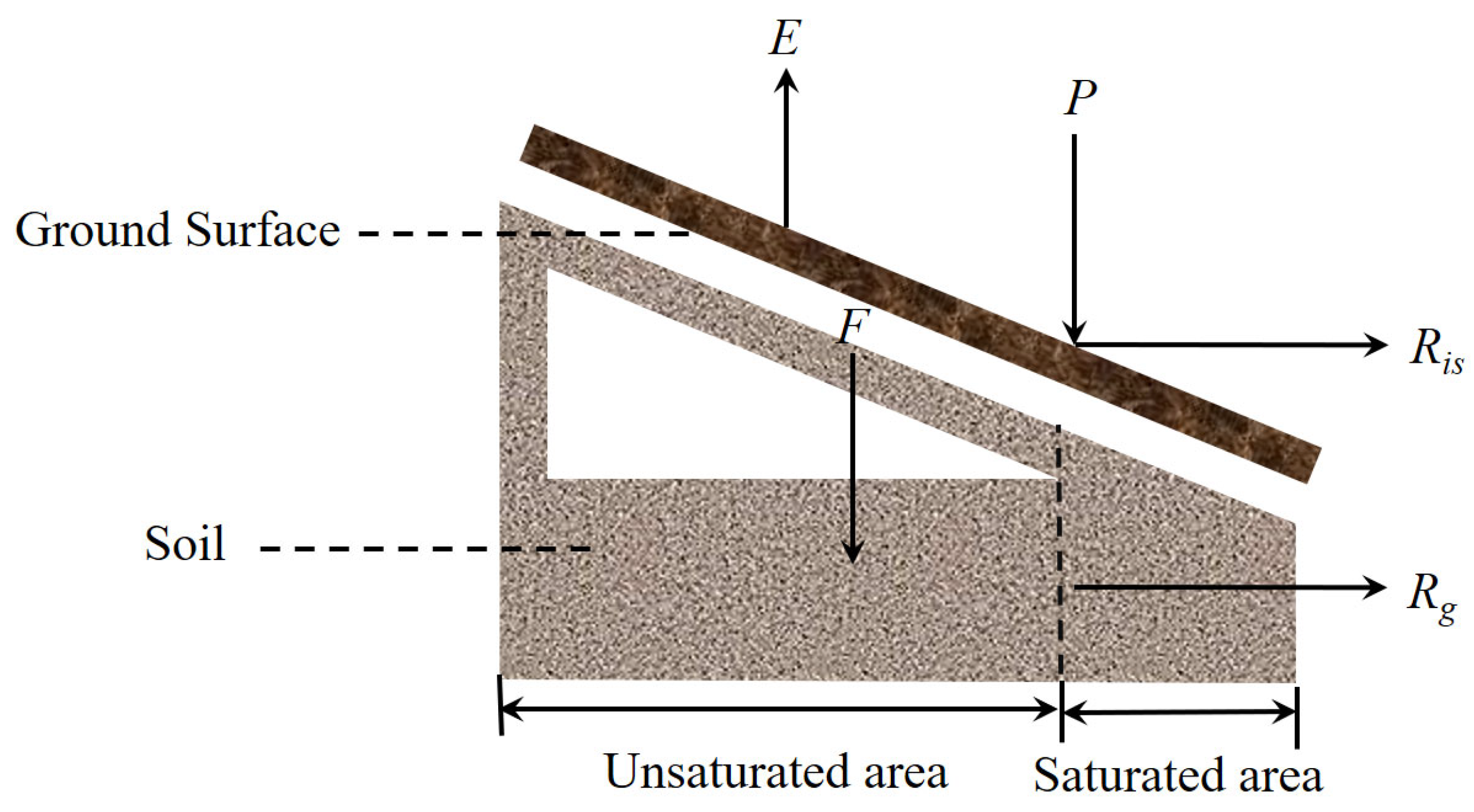
2.1. Construction of Flexible Hybrid Runoff Generation Method

At present, the well-developed and widely utilized conceptual hydrological model for saturation-excess runoff is in a mature state. However, there is still a need for a more precise comprehension of the hybrid runoff generation, particularly the challenge of distinguishing between saturation-excess and infiltration-excess runoff that coexist within a watershed in semi-humid regions. The existing prevalent hybrid runoff models are constructed in accordance with the vertical integration of saturation-excess and infiltration-excess modules, such as the Sacramento model [30].

In this study, to address this issue, we constructed a flexible hybrid runoff generation module by incorporating the vertical integration of saturation-excess and infiltration-excess modules, referring to Yi et al. [2], Huang et al. [12], and Bao and Zhao [31]. A depiction of the constructed flexible hybrid runoff generation module is shown in Figure 1, and the model fluxes are shown in

Table 1. Notations and descriptions, as well as units used in this study.

Notation	Description	Units
$P$	Rainfall	mm
$E$	Evapotranspiration	mm
$R_{is}$	Infiltration of excess surface runoff	mm
$R_g$	Saturation of excess subsurface runoff	mm
$FA$	Infiltration from the ground surface to the soil	mm

.

The hybrid runoff generation model (as shown in Figure 1) simulates the surface runoff and subsurface runoff processes. The surface runoff will be generated when the precipitation rate exceeds the infiltration rate. The surface runoff generation is simulated by combining an infiltration equation with the parabolic infiltration capacity distribution curve. The infiltration capacity distribution curve is similar to the storage capacity distribution curve within the XAJ model, which can be displayed by Equations (1) and (2).

$$\frac{A_{pi}}{A}=1-{\left(1-\frac{f_p}{f_m}\right)}^{B_1}$$

(1)

$$f_m=\overline{f}\times \left(1+B_1\right)$$

(2)

where $A_{pi}$ is the partial area where the infiltration capacity is not more than or equal to $f_p$; $f_p$ is the infiltration capacity at a point in a watershed, ranging from 0 to $f_m$; $A$ is the area of the whole watershed; $B_1$ is the exponential of distribution of the infiltration capacity; and $\overline{f}$ is the areal mean infiltration rate, which can be computed by Green–Ampt formula, Horton formula, and Philip infiltration formula, and so on [32,33,34]. In the present study, $\overline{f}$ was computed by using the Green–Ampt formula [35], which is presented as

$$f=K\left[1+\frac{\psi \mathsf{\Delta }\theta }{F}\right]$$

(3)

where $f$ is the infiltration rate (mm·h⁻¹); $F$ is the depth of the cumulative infiltration (mm); $K$ is the saturated hydraulic conductivity (mm·h⁻¹); $\psi$ is the wetting front capillary pressure head (mm); and $\mathsf{\Delta }\theta$ is the change of soil moisture content across the wetting front.

Subsurface runoff is simulated by adopting the parabolic storage capacity distribution curve [2,12], which is given by Equation (3). When the soil moisture reaches or exceeds the field capacity, subsurface runoff occurs.

$$\frac{A_{ps}}{A_p}=1-{\left(1-\frac{WM}{WMM}\right)}^{B_2}$$

(4)

where $A_{ps}$ is the partial pervious area in which the tension water storage capacity is less than or equal to the value WM, which is the tension water capacity at a point, ranging from 0 to a maximum WMM; $A_p$ is the pervious area of the watershed; and $B_2$ is the exponential of distribution of the tension water capacity.

2.2. Construction of Runoff Partition Method

The flexible hybrid runoff generation module established in Section 2.1 consists of the surface and subsurface runoffs. However, it ignores the subsurface stormflow, which is ubiquitous, especially in steep and humid watersheds. According to Huang et al. [12] and Yi et al. [2], the soil profile was separated into the upper and lower layers, and the subsurface stormflow in their model was produced between the upper and lower soil layers. Most studies have shown that subsurface stormflow is a saturated (or near-saturated) water flow phenomenon. To this end, the runoff partition method separated the subsurface stormflow from the saturation excess. In the present study, the runoff partition methods of the two-source and three-source XAJ models were introduced to the flexible runoff generation module. In addition, an improved two-source partition method was proposed to consider the heterogeneity of the subsurface topography and land covers.

2.2.1. Two-Source Runoff Partition Method

According to the original formulation in the two-source XAJ model, runoff was separated into two components using Horton’s concept of a final, constant infiltration rate ($f_c$). To this end, the steady infiltration rate was used to separate the subsurface stormflow runoff and the subsurface runoff in this study. The flow hydrograph at the outlet of the watershed was composed of the infiltration-excess surface runoff, the saturation-excess subsurface stormflow runoff, and subsurface runoff. The subsurface stormflow runoff and subsurface runoff can be expressed by

$$R_{sg}=\{\begin{array}{ll}{f}_c\frac{R_g}{FA}\hfill & PE\ge f_c\\ R_g\hfill & PE<f_c\end{array}$$

(5)

$$R_{si}=R_g-R_{sg}$$

(6)

where PE is the rainfall that exceeds evaporation; $R_{sg}$ is the saturation-excess subsurface runoff; and $R_{si}$ is the saturation-excess subsurface stormflow runoff.

2.2.2. Improved Two-Source Runoff Partition Method

The traditional two-source partition method did not consider the heterogeneity of the subsurface topography and land covers. To this end, we proposed to introduce a parabolic distribution curve to characterize the uneven distribution of the steady infiltration rate between the upper and lower soil layers. The parabolic distribution curve was analogous to the tension water storage capacity distribution curve of the XAJ model, which can be given as

$$\frac{A_{ps}}{A_p}=1-{\left(1-\frac{FM}{FMM}\right)}^{B_3}$$

(7)

where $FM$ is the steady infiltration rate at a point in a watershed, ranging from 0 to a maximum FMM, and $B_3$ is the exponential of distribution of the steady infiltration rate.

Subsequently, the subsurface stormflow runoff and subsurface runoff can be calculated according to Equation (7) and are expressed by

$$R_{si}=\{\begin{array}{ll}FR\left[FA+FM-\frac{FMM}{1+B_3}+\frac{FMM}{1+B_3}{\left(1-\frac{FA+AU}{FMM}\right)}^{1+B_3}\right]& FA+AU<FMM\\ FR\left(FA+FM-\frac{FMM}{1+B_3}\right)& FA+AU\ge FMM\end{array}$$

(8)

$$R_{sg}=\frac{R_g-R_{si}}{FR}$$

(9)

where FR, equaling to $R_g/FA$, is the proportion of the runoff-producing region over the whole watershed, and AU is the vertical coordinate corresponding to FM.

2.2.3. Three-Source Runoff Partition Method

According to the principle of hillslope hydrology, the XAJ model was adjusted to a three-source partition method to compute the runoff generation in 1992 [23]. A conceptual structure of a free water reservoir is considered based on the vertical distribution of soil moisture. More details can be found in Chen et al. [36] and Yi et al. [2]. To this end, the three-source runoff partition method was introduced to separate the total runoff of the saturation excess ($R_g$). Using the free water reservoir, the depth of the total runoff is divided into three different components, which consist of the surface runoff ($R_{ss}$), subsurface stormflow runoff ($R_{si}$), and subsurface runoff ($R_{sg}$). It is noteworthy that the surface runoff consists of both the saturation excess and infiltration excess in the flexible hybrid runoff generation models.

2.3. Hydrological Modeling Framework

In the present study, the XAJ model was utilized as the hydrological modeling framework. The XAJ model includes four modules, which are the evapotranspiration, runoff generation, runoff partition, and runoff routing modules. The saturation-excess runoff generation module of the XAJ model was substituted with the hybrid runoff generation module, and the runoff partition module was eliminated, which is named Strategy P1. Then, the runoff partition module was replaced with the two-source runoff partition module (Strategy P2), the improved two-source runoff partition module (Strategy P3), and the three-source runoff partition module (Strategy P4), respectively. The evapotranspiration and runoff routing modules remain unaltered with the current XAJ model. For detailed information on the parameters of the XAJ model, refer to Yi et al. [2]. The parameters of the runoff partition methods in the four strategies are presented in

Table 2. Parameters of the runoff partition modules for the Strategies P1, P2, P3, and P4.

Descriptions	Parameters	Strategies
		P1	P2	P3	P4
Average capacity of free water in the surface soil layer	SM (mm)	$\times$	$\times$	$\times$	$\surd$
The distribution exponent of free water capacity	B (unitless)	$\times$	$\times$	$\times$	$\surd$
Outflow coefficients of the free water storage to subsurface stormflow	KI (unitless)	$\times$	$\times$	$\times$	$\surd$
Outflow coefficients of the free water storage to subsurface flow	KG (unitless)	$\times$	$\times$	$\times$	$\surd$
Constant infiltration rate	fc (mm)	$\times$	$\surd$	$\surd$	$\times$
Exponential of the distribution to the steady infiltration rate.	B3 (unitless)	$\times$	$\times$	$\surd$	$\times$

.

Specifically, the runoff components of the four runoff partition strategies are illustrated in

Table 3. Detailed runoff components information on the four runoff partition strategies.

Runoff Components	Strategies
	P1	P2	P3	P4
Saturation-excess surface runoff	$\times$	$\times$	$\times$	$\surd$
Infiltration-excess surface runoff	$\surd$	$\surd$	$\surd$	$\surd$
Subsurface stormflow runoff	$\times$	$\surd$	$\surd$	$\surd$
Subsurface runoff	$\surd$	$\surd$	$\surd$	$\surd$

. Strategy P1 is designed to have no runoff partition module, which only consists of surface and subsurface runoff. Strategies P2, P3, and P4 consist of all three runoff components (i.e., the surface runoff, subsurface stormflow runoff, and subsurface runoff), and the differences lie in that Strategies P2 and P3 do not consider the attenuation through storage caused by the watershed, while Strategy P4 does. In addition, Strategy P4 considers the surface runoff due to the saturation-excess runoff generation mechanism.

2.4. Model Calibration and Evaluation

To optimize the parameters of the flexible hybrid runoff generation model, we used the Shuffled Complex Evolution Algorithm (SCE-UA) [28,37]. For parameter calibration, a composite objective function composed of three measurement indexes was used [2,38,39]. The composite objective function and three metrics are given as

$$E_{NS}=1-\frac{{\displaystyle {\sum }_{t=1}^T\left|Q_s^t-Q_o^t\right|}}{{\displaystyle {\sum }_{t=1}^T\left|Q_o^t-\overline{Q_o}\right|}}$$

(10)

$$E_{KG}=1-\sqrt{{\left(r-1\right)}^2+{\left(\frac{{\sigma }_s}{{\sigma }_o}-1\right)}^2+{\left(\frac{{\mu }_s}{{\mu }_o}-1\right)}^2}$$

(11)

$$R_{SR}=\sqrt{\frac{{\displaystyle {\sum }_{t=1}^T{\left(Q_o^t-Q_s^t\right)}^2}}{{\displaystyle {\sum }_{t=1}^T{\left(Q_o^t-\overline{Q_o}\right)}^2}}}$$

(12)

$$M=0.5\times \left(1-E_{\mathrm{NS}}\right)+0.25\times \left(1-E_{KG}\right)+0.15\times \left(1-\log \left(E_{NS}\right)\right)+0.1\times R_{SR}$$

(13)

where $Q_o^t$ is the measurement of discharge at time t; $Q_s^t$ is the simulation of discharge at time t; $\overline{Q_o}$ is the average value of the discharge measurement; T is the time duration of the flood event; r is the correlation coefficient between the simulated and measured flood; σ_o and σ_s are the standard deviation values for the measured and simulated responses, respectively; and μ_o and μ_s are the corresponding average values.

Several criteria were adopted for the evaluation of the model performance; these criteria consist of the E_NS, the Root Mean Square Error (RMSE), the relative flood peak error (Q_p), the relative flood peak error (W_p), as well as the flood peak time error (T_p), which can be given as

$$RMSE=\sqrt{\frac{1}{T}{\displaystyle \sum _{t=1}^T{\left(Q_s^t-Q_s^t\right)}^2}}$$

(14)

$$Q_p=\frac{Q_p^s-Q_p^o}{Q_p^o}$$

(15)

$$W_p=\frac{{\displaystyle {\sum }_{t=1}^T{W}_s^t}-{\displaystyle {\sum }_{t=1}^T{W}_o^t}}{{\displaystyle {\sum }_{t=1}^T{W}_o^t}}$$

(16)

$$T_p=T_p^s-T_p^o$$

(17)

where $Q_p^o$ is the measurement of flood peak discharge; $Q_p^s$ is the simulation of flood peak discharge; $Q_o^t$ is the measurement of flood volume at time t; $Q_s^t$ is the simulation of flood volume at time t; $T_p^o$ is the measurement of flood peak time; and $T_p^s$ is the simulation of flood peak time.

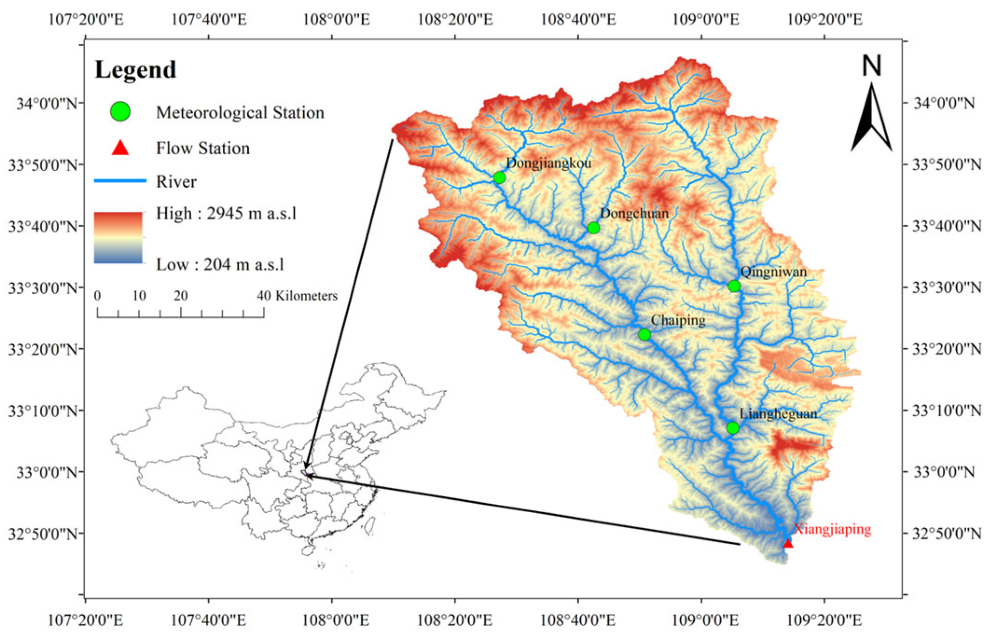
3. Study Area and Data

As an important tributary of the Han River, the Xun River is situated in Shaanxi Province, China. Its length is 218 km. The basin area is 6448 km². The average slope of the whole watershed amounts to 2.9‰. The Xun River basin is situated in mountainous terrain with significant variations in topographic relief, in which the runoff generation heterogeneity characteristics of the watershed should be taken into account in the processes of hydrological modeling. The Xun River basin is located in the transition zone between the warm temperate and the northern subtropical regions. It experiences low rainfall in winter, with an average temperature of 7.8 °C. In contrast, it receives abundant rainfall during summer with an average temperature of 24.8 °C. The average annual rainfall is 798 mm in the entire basin. The flood season occurs from July to October, which accounts for 60% of the total annual runoff.

As depicted in Figure 2, the basin contains one flow station (the Xiangjiaping Station) and six meteorological stations. As the outlet of the Xun River basin, the Xiangjiaping hydrological station has an annual average discharge of 63.4 m³/s. The highest recorded flood peak discharge at the basin outlet stands at 6090 m³/s. Floods in the Xun River basin are typically characterized by short durations and high flow peaks, posing significant threats to downstream areas. Consequently, relying solely on a single runoff generation mechanism for watershed flood prediction in this basin is insufficient, and hybrid runoff generation mechanisms are to be constructed urgently.

The meteorological stations provided the six-hourly rainfall and evapotranspiration data spanning from 2010 to 2021. Additionally, we collected the six-hourly runoff data at the Xiangjiaping Station during the same period. To calibrate and validate the constructed model, we specifically chose the annual flow series during the flood seasons. The period from 2010 to 2017 is used for calibration, and the period from 2018 to 2021 is used for validation. However, we excluded the flood season of 2016 due to a significant error in the measured flow discharge. In addition, we identified 23 flood events with flood peak discharge exceeding 500 m³/s. Both the calibration and validation periods aligned with the continuous flow discharge data. Moreover, we calculated the antecedent precipitation by using the daily recession coefficient of the water storage, taking into account the initial condition.

4. Results

4.1. Model Calibration and Performance Evaluation for the Continuous Flow Discharge

This study used the XAJ model as the hydrological forecasting framework, replacing the saturation-excess runoff generation module with a hybrid runoff generation module. We designed four runoff partition strategies to explore the effects of the runoff partition method over the flexible hybrid runoff generation model for flood prediction. The other modules remained unaltered within the original XAJ model. The continuous discharge processes in the flood season from 2010 to 2017 were adopted to calibrate the established hydrological model, while the rest were used for validation. Several evaluation indices, including E_NS, E_KG, and RMSE, were adopted to evaluate the performances of different runoff partition strategies, as listed in

Table 4. Performances of the four runoff partition strategies of the Xun River basin.

Criteria	Strategies	Calibration Period							Validation Period
		2010	2011	2012	2013	2014	2015	2017	2018	2019	2020	2021
ENS	P1	0.75	0.81	0.59	0.70	0.67	0.38	0.84	0.55	0.73	0.56	0.74
	P2	0.78	0.85	0.65	0.70	0.69	0.49	0.84	0.67	0.76	0.68	0.80
	P3	0.77	0.87	0.66	0.70	0.73	0.48	0.85	0.60	0.81	0.72	0.82
	P4	0.78	0.85	0.68	0.73	0.72	0.48	0.85	0.58	0.78	0.69	0.81
EKG	P1	0.59	0.88	0.61	0.69	0.74	0.65	0.68	0.40	0.86	0.64	0.79
	P2	0.68	0.85	0.64	0.80	0.80	0.66	0.67	0.51	0.88	0.77	0.82
	P3	0.68	0.87	0.64	0.83	0.83	0.66	0.67	0.44	0.89	0.79	0.83
	P4	0.69	0.87	0.64	0.83	0.83	0.69	0.68	0.41	0.88	0.77	0.83
RMSE	P1	132.5	192.6	108.8	56.2	201.6	81.2	122.2	103.2	133.6	74.7	231.7
	P2	123.2	175.5	100.6	56.3	193.1	73.3	120.9	87.8	125.5	64.0	202.9
	P3	126.0	160.9	99.3	55.7	181.1	74.1	118.5	96.6	112.9	59.2	194.6
	P4	123.1	174.7	97.1	53.0	183.6	74.0	115.6	99.6	122.3	62.8	200.0

. Figure 3 shows the discharge hydrographs of the four runoff partition methods, in which the calibration years are 2010, 2011, and 2017, and the validation years are 2019, 2020, and 2021.

The average E_NS of the Strategies P1, P2, P3, and P4 are 0.67, 0.72, 0.73, and 0.72; the average E_KG are 0.68, 0.73, 0.74, and 0.74; and the average RMSE is 130.75, 120.28, 116.26, and 118.71 m³/s, respectively. It can be observed from Table 4 and Figure 3 that Strategy P1 is the poorest in performance. The performances of Strategies P2, P3, and P4 are almost consistent, and the performances of Strategies P3 and P4 are slightly better than that of Strategy P2. However, model complexity control is necessary as the model with more parameters can have higher precision in most cases [40]. The number of parameters of partition methods in Strategies P2, P3, and P4 are 1, 2, and 4, respectively. To this end, it is difficult to determine which strategy can reflect the actual conditions of the natural watershed. Figure 4 presents the density distribution of the measured and simulated discharge hydrographs in order to demonstrate the performances of different strategies more visually.

Figure 4 plots the density distribution curves for the measured discharge and simulated discharge hydrographs of the four strategies. The results show that the density curves of the four strategies are similar to that of the measured discharge besides 2020. Similar to the results in Table 4, the performances of the simulated results in 2011, 2019, and 2021 are the best. As shown in Figure 4a,b, the results demonstrate that the simulated results are lower than the measured discharge when the actual discharge is high. The errors in 2020 are large, possibly because the discharge in 2020 is lower than those of the other years. In addition, it can also be observed from Figure 4 that the density distribution curves of Strategy P2 are more consistent with that of the measured discharge.

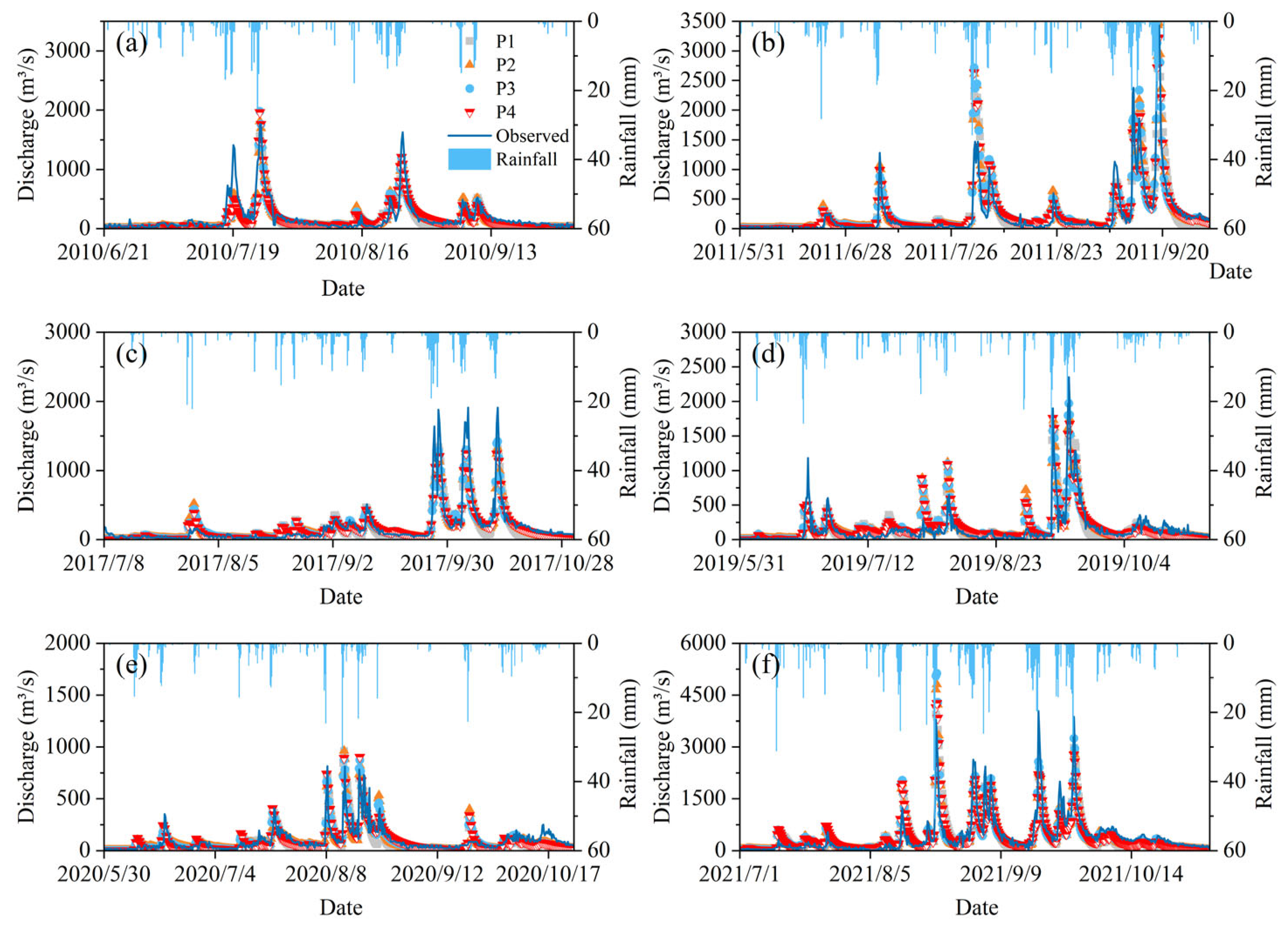
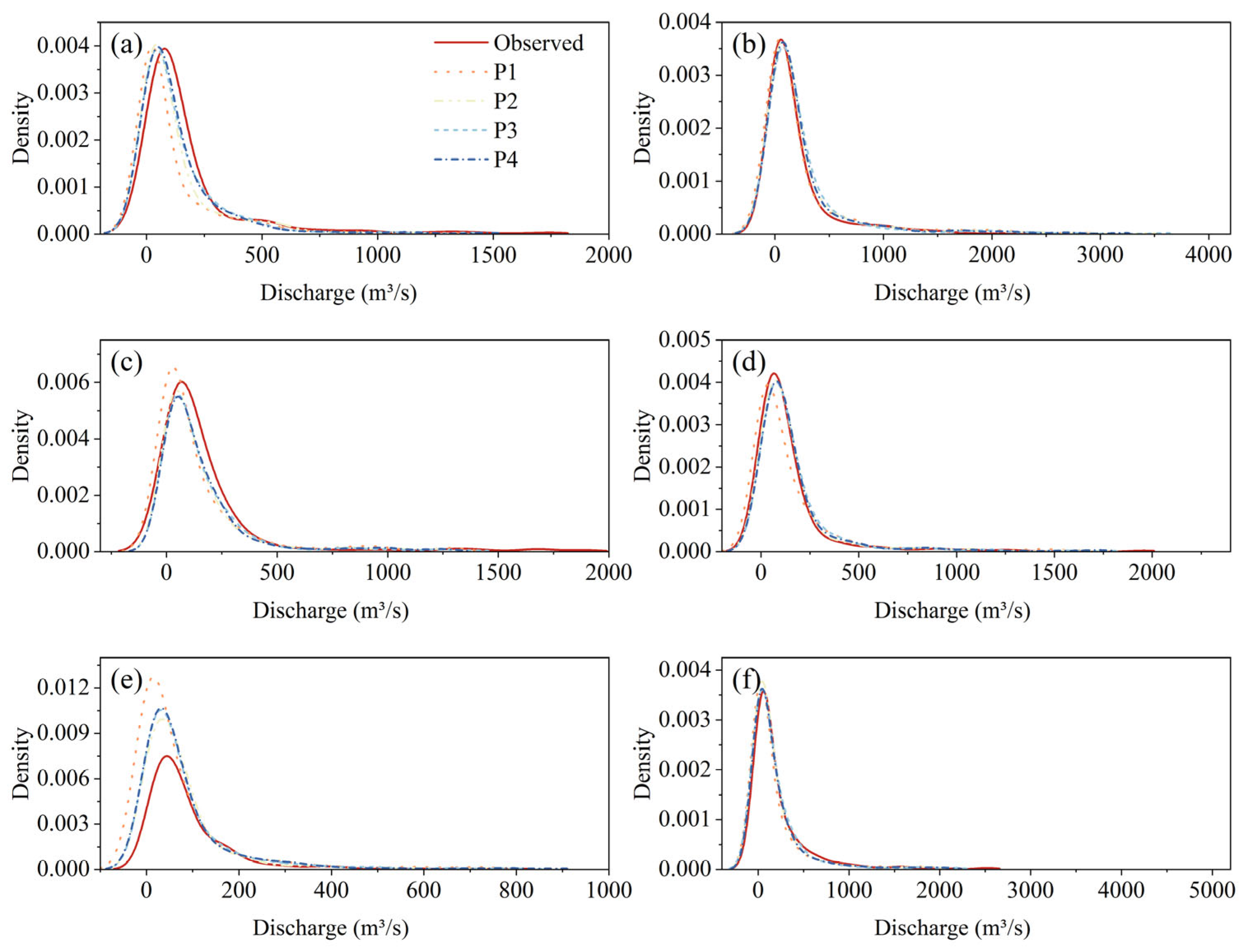
4.2. Performances of Simulated Results of Flood Events

Depending on the application, hydrological modeling can be event-based or continuous [41]. Individual flood events are simulated by event-based models. Mostly, we focus on flood events because of their extensive damage. To this end, 23 flood events were selected from the continuous flow discharge process from 2010 to 2021 to further analyze the performances of flood events.

It is noteworthy that the hydrological models’ parameters for both the flood events and the continuous flow discharge were calibrated together. The discharge peak, discharge volume, discharge process, and occurrence time of discharge peak are the four essential elements to describe the discharge hydrograph, and the evaluation index distributions are plotted in Figure 5.

Figure 5 demonstrates the distributions of the evaluation index, which includes Q_p, T_p, E_NS, and W_p. The results are consistent with those of the continuous flow discharge. Strategies P3 and P4 outperformed the other strategies, followed by Strategy P2. Specifically, the E_NS of Strategies P3 and P4 have a more centralized distribution, demonstrating that the models are more robust than others. The T_p distributions of the four strategies are almost the same. The Q_p and W_p distributions of Strategies P3 and P4 are slightly better than those of Strategies P1 and P2. Overall, the hydrological models’ performances with runoff partition modules are better than Strategy P1. Although Strategy P4 introduced four parameters to describe the runoff partition module, it did not perform as satisfactorily as expected. Therefore, quantitative studies are needed to determine the differences in the four runoff partition strategies and further explore their influences on the performances of the flexible hybrid runoff generation model.

4.3. Comparisons of Runoff Components for the Four Runoff Partition Strategies

In order to explore the quantitative influences of the runoff partition method on the flexible hybrid runoff generation model for flood prediction, we analyze the three runoff components of the four runoff partition strategies. Figure 6 plots the runoff components computed by the four runoff partition strategies for the flow discharge processes in 2010, 2011, 2017, 2019, 2020, and 2021.

It can be observed from Figure 6 that the proportions of each runoff component for the four strategies are significantly different, while the proportion of subsurface runoff for all strategies is high. Since the runoff partition module was not considered, Strategy P1 consists of only surface and subsurface runoffs, and its results are different from other strategies in that the subsurface runoff occupies about 80% of the total runoff. Strategies P2, P3, and P4 contain all three runoff components, while the proportion of the subsurface stormflow runoff of Strategy P4 is tiny, with surface runoff and subsurface runoff each occupying about 50%. Strategy P2 has the highest percentage of subsurface stormflow runoff of all strategies. Based on our previous research [2], the Xun River basin has abundant subsurface stormflow runoff, accounting for about 30% of the total runoff. We noted that the results of component ratios of Strategy P3 are the most consistent with our previous research.

5. Discussion

5.1. Discussion on Model Performance and Applicability

It is noteworthy that although the ratios of runoff components are significantly different, Strategies P3 and P4 show almost consistent performances, which indeed raised an issue on the parameter equifinality [42].

We tried to analyze the differences between each strategy theoretically. For Strategies P2 and P3, the two-source runoff partition methods are used to divide the infiltration into subsurface stormflow and subsurface runoffs. The differences lie in that Strategy P3 considers the heterogeneity of the steady infiltration of the watershed, and the results show that Strategy P3 performed a lot better than Strategy P2. However, it is noteworthy that Strategy P3 performs consistently with Strategy P4, even though Strategy P4 has a larger number of parameters. Generally speaking, complex models are more likely to achieve better simulation results than simple models, but this does not mean that complex models can accurately reflect the actual hydrological conditions of a watershed. To this end, the physical mechanism of Strategy P4 deserves further clarification and exploration.

The three-source runoff partition method adopted in Strategy P4 has been widely used in the XAJ hydrological model [36,43,44]. Unlike the flexible hybrid runoff generation model used in this study, the XAJ model operates based on the saturation-excess runoff generation mechanism, resulting in surface runoff when there is no available soil moisture storage [45]. This is significantly different from the constructed flexible hybrid runoff generation model used in this study, in which the surface runoff occurs when the precipitation rate exceeds the saturated hydraulic conductivity of the surface soil [2]. When Strategy P4 is adopted to separate the excess rainfall, the surface runoff consists of both the saturation-excess and infiltration-excess runoffs.

In addition, it is still not specific whether it is reasonable to consider both the saturated- and infiltrated-surface runoffs in a hydrological model. Bao et al. proposed an improved Green–Ampt infiltration equation, which is related to the storage of soil moisture [35,46]. Since the infiltration equation considers the influence of the soil moisture storage, the infiltration-excess surface runoff computed using the infiltration equation can be explained by the saturation-excess runoff generation and the infiltration-excess runoff generation mechanisms [47,48]. For this reason, the saturation-excess surface runoff should not be recalculated doubly.

In summary, we designed four strategies to investigate the influences of the runoff partition method on the flexible hybrid runoff generation model for flood prediction. The simulation results demonstrated that the runoff partition method was critical to the flexible runoff generation model. Contrary to common perceptions, Strategy P4 did not perform exceptionally well, and it could not reflect the real conditions of the reality of the watershed. Strategy P4 overestimated the surface runoff and almost ignored the subsurface stormflow runoff. Strategies P2 and P3 showed good performances and, considering the heterogeneity of steady infiltration, could improve the simulation of the discharge hydrographs at the outlet of the watershed.

5.2. Discussion on the Nonlinear Components of the Four Strategies

As we discussed in the Section 1, the flexible hybrid runoff hydrological models allowed for the selection of alternative representations of runoff processes and various combinations of both linear and nonlinear components. The nonlinear components of each sub-modules can significantly improve the performance of the hydrological model [49,50]. There are 2, 2, 3, and 3 nonlinear components of the four strategies, respectively. In Strategies P1 and P2, the key nonlinear components are the distribution curves of infiltration capacity as well as soil moisture storage capacity in a parabolic manner, and their shapes are determined by two shape parameters, B₁ and B₂, respectively. In Strategies P3, we proposed a third nonlinear component, namely the steady infiltration capacity distribution curve over the interface, to divide the infiltration from the upper soil into the subsurface stormflow runoff and the subsurface runoff. Simultaneously, the shape of the curve was characterized by a shape parameter, B₃. In Strategy P4, the free water storage reservoir was introduced to separate the three runoff components from infiltration.

It is unreasonable to compare models with different degrees of flexibility, and it is obvious that the hydrological model with a higher degree of flexibility is more likely to perform better than those with a low degree of flexibility [12]. This conclusion is consistent with the results in Section 4.1 and Section 4.2. The high flexibility of those nonlinear components in Strategies P3 and P4 may answer why both the models have better performances than Strategies P1 and P2 in the study case. For Strategies P3 and P4, the performances of these two strategies show similar results, while the runoff components are significantly different. This phenomenon has been discussed in Section 5.1.

The above discussions demonstrate that enough key nonlinear components are necessary to accommodate complex and diverse hydrological environments. Simultaneously, Huang et al. [12] argued that the nonlinear components ought to possess enough flexibility. In addition, we found that the complex model does not necessarily reflect the actual condition of the real watershed, and the improvement of the model’s performances can be due to the complexity of the modeling structure or the increase in the number of parameters.

6. Conclusions

We constructed the flexible hybrid runoff generation models by combining the saturation-excess runoff generation and infiltration-excess runoff generation mechanisms and used the XAJ model as the hydrological modeling framework in this study. We designed four strategies to investigate the influences of the runoff partition method on the flexible hybrid runoff generation model for flood prediction. Performances of various runoff partition methods, which consist of the two-source, improved two-source, and three-source methods, were compared and discussed based on the continuous flow discharge and flood events. In addition, the model performances and applicability, as well as the nonlinear components of the four strategies, were discussed. The main conclusions are summarized as follows:

(1)

Strategy P3 and P4 outperform other strategies, followed by Strategy S2. And Strategy P1 with no runoff partition module cannot reflect the actual conditions of the watershed;

(2)

Although the performance of Strategy P4 is good, it is not applicable to the flexible hybrid runoff generation models because it overestimates the surface runoff and almost ignores the subsurface stormflow runoff;

(3)

Strategy P3 is a compromise between strategies P2 and P4. It retains the advantages of the free reservoir in Strategy P4 and considers the heterogeneity of the watershed;

(4)

The runoff partition method is of great influence on the performances of the flexible hybrid runoff generation model. Given that most watersheds are dominated by a mixed runoff generation mechanism rather than a single runoff generation mechanism, our study has great practical value for hydrological modeling and flood prediction.

References

1. Zhang, L.; Hu, C.; Jian, S.; Wu, Q.; Ran, G.; Xu, Y. Identifying dominant component of runoff yield processes: A case study in a sub-basin of the middle Yellow River. Hydrol. Res. 2021, 52, 1033–1047. [Google Scholar] [CrossRef]
2. Yi, B.; Chen, L.; Liu, Y.; Guo, H.; Leng, Z.; Gan, X.; Xie, T.; Mei, Z. Hydrological modelling with an improved flexible hybrid runoff generation strategy. J. Hydrol. 2023, 620, 129457. [Google Scholar] [CrossRef]
3. Shen, Y.J.; Liu, D.D.; Yin, J.B.; Xiong, L.H.; Liu, P. Integrating hybrid runoff generation mechanism into variable infiltration capacity model to facilitate hydrological simulations. Stoch. Environ. Res. Risk Assess. 2020, 34, 2139–2157. [Google Scholar] [CrossRef]
4. Wang, W.; Liu, J.; Xu, B.; Li, C.; Liu, Y.; Yu, F. A WRF/WRF-Hydro coupling system with an improved structure for rainfall-runoff simulation with mixed runoff generation mechanism. J. Hydrol. 2022, 612, 128049. [Google Scholar] [CrossRef]
5. Liu, Y.; Zhang, K.; Li, Z.; Liu, Z.; Wang, J.; Huang, P. A hybrid runoff generation modelling framework based on spatial combination of three runoff generation schemes for semi-humid and semi-arid watersheds. J. Hydrol. 2020, 590, 125440. [Google Scholar] [CrossRef]
6. Yao, C.; Zhang, K.; Yu, Z.; Li, Z.; Li, Q. Improving the flood prediction capability of the Xinanjiang model in ungauged nested catchments by coupling it with the geomorphologic instantaneous unit hydrograph. J. Hydrol. 2014, 517, 1035–1048. [Google Scholar] [CrossRef]
7. Li, Z.J.; Yao, C.; Kong, X.G. The Improved Xinanjiang model. J. Hydrodyn. Ser. B 2005, 17, 746–751. [Google Scholar] [CrossRef]
8. Bao, W.; Wang, C. Vertically-mixed runoff model and its application. Hydrology 1997, 3, 18–21. [Google Scholar] [CrossRef]
9. Liang, X.; Xie, Z. A new surface runoff parameterization with subgrid-scale soil heterogeneity for land surface models. Adv. Water Resour. 2001, 24, 1173–1193. [Google Scholar] [CrossRef]
10. Euser, T.; Winsemius, H.C.; Hrachowitz, M.; Fenicia, F.; Uhlenbrook, S.; Savenije, H.H.G. A framework to assess the realism of model structures using hydrological signatures. Hydrol. Earth Syst. Sci. 2013, 17, 1893–1912. [Google Scholar] [CrossRef] [Green Version]
11. Zhang, K.; Xue, X.; Hong, Y.; Gourley, J.J.; Lu, N.; Wan, Z.; Hong, Z.; Wooten, R. iCRESTRIGRS: A coupled modeling system for cascading flood–landslide disaster forecasting. Hydrol. Earth Syst. Sci. 2016, 20, 5035–5048. [Google Scholar] [CrossRef] [Green Version]
12. Huang, P.N.; Li, Z.J.; Chen, J.; Li, Q.L.; Yao, C. Event-based hydrological modeling for detecting dominant hydrological process and suitable model strategy for semi-arid catchments. J. Hydrol. 2016, 542, 292–303. [Google Scholar] [CrossRef]
13. Bai, P.; Liu, X.; Yang, T.; Liang, K.; Liu, C. Evaluation of streamflow simulation results of land surface models in GLDAS on the Tibetan plateau. J. Geophys. Res. Atmos. 2016, 121, 12180–12197. [Google Scholar] [CrossRef]
14. Qi, J.; Lee, S.; Zhang, X.; Yang, Q.; McCarty, G.W.; Moglen, G.E. Effects of surface runoff and infiltration partition methods on hydrological modeling: A comparison of four schemes in two watersheds in the Northeastern US. J. Hydrol. 2020, 581, 124415. [Google Scholar] [CrossRef]
15. Kling, H.; Nachtnebel, H.P. A method for the regional estimation of runoff separation parameters for hydrological modelling. J. Hydrol. 2009, 364, 163–174. [Google Scholar] [CrossRef]
16. Haberlandt, U.; Klöcking, B.; Krysanova, V.; Becker, A. Regionalisation of the base flow index from dynamically simulated flow components—A case study in the Elbe River Basin. J. Hydrol. 2001, 248, 35–53. [Google Scholar] [CrossRef]
17. Naef, F.; Scherrer, S.; Weiler, M. A process based assessment of the potential to reduce flood runoff by land use change. J. Hydrol. 2002, 267, 74–79. [Google Scholar] [CrossRef]
18. Gurtz, J.; Zappa, M.; Jasper, K.; Lang, H.; Verbunt, M.; Badoux, A.; Vitvar, T. A comparative study in modelling runoff and its components in two mountainous catchments. Hydrol. Process. 2003, 17, 297–311. [Google Scholar] [CrossRef]
19. Ardekani, A.A.; Sabzevari, T.; Haghighi, A.T.; Petroselli, A. Separation of surface flow from subsurface flow in catchments using runoff coefficient. Acta Geophys. 2021, 69, 2363–2376. [Google Scholar] [CrossRef]
20. Maier, F.; van Meerveld, I.; Weiler, M. Long-Term Changes in Runoff Generation Mechanisms for Two Proglacial Areas in the Swiss Alps II: Subsurface Flow. Water Resour. Res. 2021, 57, e2021WR030223. [Google Scholar] [CrossRef]
21. Wu, J.; Li, H.; Zhou, J.; Tai, S.; Wang, X. Variation of Runoff and Runoff Components of the Upper Shule River in the Northeastern Qinghai&ndash;Tibet Plateau under Climate Change. Water 2021, 13, 3357. [Google Scholar] [CrossRef]
22. Appels, W.M.; Bogaart, P.W.; van der Zee, S.E.A.T.M. Feedbacks Between Shallow Groundwater Dynamics and Surface Topography on Runoff Generation in Flat Fields. Water Resour. Res. 2017, 53, 10336–10353. [Google Scholar] [CrossRef] [Green Version]
23. Zhao, R.J. The Xinanjiang model applied in China. J. Hydrol. 1992, 135, 371–381. [Google Scholar] [CrossRef]
24. Kirkby Mike, J. Hillslope form and process: History 1960–2000+. Geol. Soc. Lond. Mem. 2022, 58, 213–225. [Google Scholar] [CrossRef]
25. Li, H.; Zhang, Y.; Chiew, F.H.S.; Xu, S. Predicting runoff in ungauged catchments by using Xinanjiang model with MODIS leaf area index. J. Hydrol. 2009, 370, 155–162. [Google Scholar] [CrossRef]
26. Tong, B.; Li, Z.; Yao, C.; Wang, J.; Huang, Y. Derivation of the Spatial Distribution of Free Water Storage Capacity Based on Topographic Index. Water 2018, 10, 1407. [Google Scholar] [CrossRef] [Green Version]
27. Hao, F.; Sun, M.; Geng, X.; Huang, W.; Ouyang, W. Coupling the Xinanjiang model with geomorphologic instantaneous unit hydrograph for flood forecasting in northeast China. Int. Soil Water Conserv. Res. 2015, 3, 66–76. [Google Scholar] [CrossRef] [Green Version]
28. Zhou, Q.; Chen, L.; Singh, V.P.; Zhou, J.; Chen, X.; Xiong, L. Rainfall-runoff simulation in karst dominated areas based on a coupled conceptual hydrological model. J. Hydrol. 2019, 573, 524–533. [Google Scholar] [CrossRef]
29. Pelletier, A.; Andréassian, V. Hydrograph separation: An impartial parametrisation for an imperfect method. Hydrol. Earth Syst. Sci. 2020, 24, 1171–1187. [Google Scholar] [CrossRef] [Green Version]
30. Huang, P.; Li, Z.; Yao, C.; Li, Q.; Yan, M. Spatial Combination Modeling Framework of Saturation-Excess and Infiltration-Excess Runoff for Semihumid Watersheds. Adv. Meteorol. 2016, 2016, 5173984. [Google Scholar] [CrossRef] [Green Version]
31. Bao, W.; Zhao, L. Application of Linearized Calibration Method for Vertically Mixed Runoff Model Parameters. J. Hydrol. Eng. 2014, 19, 04014007. [Google Scholar] [CrossRef]
32. Green, W.H.; Ampt, G.A. Studies on soil physics. The flow of air and water through soils. J. Agric. Sci. 1911, 4, 11–24. [Google Scholar] [CrossRef]
33. Philip, J.R. The theory of infiltration: 4. Sorptivity and algebraic infiltration equations. Soil Sci. 1957, 84, 257–264. [Google Scholar] [CrossRef]
34. Beven, K.; Robert, E. Horton’s perceptual model of infiltration processes. Hydrol. Process. 2004, 18, 3447–3460. [Google Scholar] [CrossRef]
35. Huo, W.B.; Li, Z.J.; Zhang, K.; Wang, J.F.; Yao, C. GA-PIC: An improved Green-Ampt rainfall-runoff model with a physically based infiltration distribution curve for semi-arid basins. J. Hydrol. 2020, 586, 124900. [Google Scholar] [CrossRef]
36. Chen, Y.; Shi, P.; Qu, S.; Ji, X.; Zhao, L.; Gou, J.; Mou, S. Integrating XAJ Model with GIUH Based on Nash Model for Rainfall-Runoff Modelling. Water 2019, 11, 772. [Google Scholar] [CrossRef] [Green Version]
37. Duan, Q.; Sorooshian, S.; Gupta, V. Effective and efficient global optimization for conceptual rainfall-runoff models. Water Resour. Res. 1992, 28, 1015–1031. [Google Scholar] [CrossRef]
38. Brunner, M.I.; Swain, D.L.; Wood, R.R.; Willkofer, F.; Done, J.M.; Gilleland, E.; Ludwig, R. An extremeness threshold determines the regional response of floods to changes in rainfall extremes. Commun. Earth Environ. 2021, 2, 173. [Google Scholar] [CrossRef]
39. Yi, B.; Chen, L.; Zhang, H.; Singh, V.P.; Jiang, P.; Liu, Y.; Guo, H.; Qiu, H. A time-varying distributed unit hydrograph method considering soil moisture. Hydrol. Earth Syst. Sci. 2022, 26, 5269–5289. [Google Scholar] [CrossRef]
40. Pilz, T.; Francke, T.; Baroni, G.; Bronstert, A. How to Tailor My Process-Based Hydrological Model? Dynamic Identifiability Analysis of Flexible Model Structures. Water Resour. Res. 2020, 56, e2020WR028042. [Google Scholar] [CrossRef]
41. Katwal, R.; Li, J.; Zhang, T.; Hu, C.; Rafique, M.A.; Zheng, Y. Event-based and continous flood modeling in Zijinguan watershed, Northern China. Nat. Hazards 2021, 108, 733–753. [Google Scholar] [CrossRef]
42. Beven, K. A manifesto for the equifinality thesis. J. Hydrol. 2006, 320, 18–36. [Google Scholar] [CrossRef] [Green Version]
43. Wang, J.; Wang, G.; Elmahdi, A.; Bao, Z.; Yang, Q.; Shu, Z.; Song, M. Comparison of hydrological model ensemble forecasting based on multiple members and ensemble methods. Open Geosci. 2021, 13, 401–415. [Google Scholar] [CrossRef]
44. Hao, G.; Li, J.; Song, L.; Li, H.; Li, Z. Comparison between the TOPMODEL and the Xin’anjiang model and their application to rainfall runoff simulation in semi-humid regions. Environ. Earth Sci. 2018, 77, 279. [Google Scholar] [CrossRef]
45. Li, D.; Liang, Z.; Zhou, Y.; Li, B.; Fu, Y. Multicriteria assessment framework of flood events simulated with vertically mixed runoff model in semiarid catchments in the middle Yellow River. Nat. Hazards Earth Syst. Sci. 2019, 19, 2027–2037. [Google Scholar] [CrossRef] [Green Version]
46. Gowdish, L.; Muñoz-Carpena, R. An Improved Green–Ampt Infiltration and Redistribution Method for Uneven Multistorm Series. Vadose Zone J. 2009, 8, 470–479. [Google Scholar] [CrossRef]
47. Liu, Y.; Cui, Z.; Huang, Z.; López-Vicente, M.; Wu, G.-L. Influence of soil moisture and plant roots on the soil infiltration capacity at different stages in arid grasslands of China. CATENA 2019, 182, 104147. [Google Scholar] [CrossRef]
48. Yang, M.; Zhang, Y.; Pan, X. Improving the Horton infiltration equation by considering soil moisture variation. J. Hydrol. 2020, 586, 124864. [Google Scholar] [CrossRef]
49. Basu, B.; Morrissey, P.; Gill, L.W. Application of Nonlinear Time Series and Machine Learning Algorithms for Forecasting Groundwater Flooding in a Lowland Karst Area. Water Resour. Res. 2022, 58, e2021WR029576. [Google Scholar] [CrossRef]
50. Ghonchepour, D.; Sadoddin, A.; Bahremand, A.; Croke, B.; Jakeman, A.; Salmanmahiny, A. A methodological framework for the hydrological model selection process in water resource management projects. Nat. Resour. Model. 2021, 34, e12326. [Google Scholar] [CrossRef]
Figure 1. Depiction of the flexible runoff generation module.
Water 15 02738 g001
Figure 2. Locations of the flow and meteorological stations in the Xun River basin.
Water 15 02738 g002
Figure 3. Discharge hydrographs obtained by the four runoff partition strategies. (a) Discharge hydrographs in 2010. (b) Discharge hydrographs in 2011. (c) Discharge hydrographs in 2017. (d) Discharge hydrographs in 2019. (e) Discharge hydrographs in 2020. (f) Discharge hydrographs in 2021.
Water 15 02738 g003
Figure 4. Density distribution of the measured and simulated discharge hydrographs: (a) Density distribution curve in 2010. (b) Density distribution curve in 2011. (c) Density distribution curve in 2017. (d) Density distribution curve in 2019. (e) Density distribution curve in 2020. (f) Density distribution curve in 2021.
Water 15 02738 g004
Figure 5. Distributions of evaluation index with different runoff partition strategies for flood events. (a) Distribution of Qp. (b) Distribution of Tp. (c) Distribution of ENS. (d) Distribution of Wp.
Water 15 02738 g005
Figure 6. Stacked bar charts of runoff components for the four runoff partition strategies. (a) 2010. (b) 2011. (c) 2017. (d) 2019. (e) 2020. (f) 2021.
Water 15 02738 g006