Article

Hydrokinetic Energy and Transient Accelerations of Marine Currents in Colombian Nearshore Waters

by
Juan Gabriel Rueda-Bayona
1,2,*,
Juan José Cabello Eras
3,
Ana Lucía Caicedo-Laurido
4,
Andrés Guzmán
5 and
José Luis García Vélez
1,2
1
Natural and Environmental Resources Engineering School (EIDENAR), Faculty of Engineering, Universidad del Valle, Cali 760042, Colombia
2
INCIMAR Institute of Marine Sciences and Limnology, Universidad del Valle, Cali 760042, Colombia
3
Departamento de Ingeniería Mecánica, Facultad de Ingeniería, Universidad de Córdoba, Carrera 6 No. 77-305, Montería 230002, Colombia
4
Dirección General Marítima, Bogotá 111711, Colombia
5
Research Group for Structures and Geotechnics (GIEG), Department of Civil and Environmental Engineering, Universidad del Norte, Km 5 Via Puerto Colombia, Bloque K, 8-33K, Barranquilla 080020, Colombia
*
Author to whom correspondence should be addressed.
Water 2023, 15(15), 2725; https://doi.org/10.3390/w15152725
Submission received: 8 May 2023 / Revised: 12 July 2023 / Accepted: 19 July 2023 / Published: 28 July 2023
(This article belongs to the Section Oceans and Coastal Zones)

Abstract

:
The transient acceleration of ocean currents, or internal waves, is hard to detect, because it does not have climate variability or regular manifestation in the sea. This fluctuation affects not only short-term oceanographic processes but also the hydrokinetic generation of power and the structural health of ocean technologies. Identifying and understanding the mechanisms that generate internal waves require long-term data on the kinetic and viscous–turbulent parameters of the water column measured over long intervals. In this sense, this study analyzed current profiles in nearshore waters (8.9 m depths) measured over six months in the Colombian Caribbean Sea and found internal waves due to the manifestation of transient acceleration propagating in two of the three layers of the water column. The analyzed time series of currents and turbulent kinetic profiles evidenced that transient waves occurred during changes in the surface winds. The applied methodology in this research allowed, for the first time in the study area, the detection of transient accelerations (±0.25 m/s2) that modified the hydrokinetic energy of the water column over short-term periods (6–24 h).

1. Introduction

The effect of greenhouse gases (GHGs) on the Earth have been identified in climate change [1] and sea level rise [2], which are provoking problems in the environment, human health and social interactions [3,4,5]. As a result, the need to reduce the copious amounts of GHGs generated by the current carbonized economy demands a rapid energy transition. Renewables, as an alternative to decarbonize the energy sector, have shown to be a significant technological development over the last decades because of the progress in wind and photovoltaic technologies [6]. However, other renewable energy technologies require more research and development in order for their use to spread, such as marine energies [7]. Wave power and marine current energy depend on the interaction of winds, waves, and sea currents, where the energy conversion from kinetic potential depends on the water depth and sea state transitions [8]. Low sea states are characterized by significantly reduced wave heights (Hs < 1 m), which are frequently not considered for offshore structure design despite it being proven that low sea states generate significant transient current accelerations that can affect the structural health of marine technologies [9,10].
From an energy extraction perspective, transient current accelerations must be treated like transitory events, the same as gusts are for wind energy, because turbulent and rapid changes in fluid flow affect the performance and integrity of turbines [11]. Similarly, transient marine currents have a similar effect on marine energy production as transient wind gust does on wind energy because unexpected changes in current velocities (i.e., nonlinear and turbulent) over short-term periods affect the hydrodynamic field [12,13]. The design and optimization of hydrokinetic turbines [13,14] and wave power converters [7] should consider these transient changes in the local hydrodynamics generated during low sea states. The generation of transient current accelerations has been identified in internal solitary waves through ADCP (acoustic Doppler current profilers) measurements [15], where kinetic and viscous parameters have been analyzed [16]. The internal solitary waves convey transient accelerations, which vary along the water column and provoke torque and forces over the structures [17,18].
The Colombian Caribbean coast is considered a region with significant availability of offshore wind [19] and wave power energy [20], where mesoscale climate events affect energy source dynamics [21,22]. Marine currents have not yet been characterized for energy purposes in the nearshore areas of the Colombian Caribbean, but there exist reports of marine currents for marine energy extraction in deep waters [23]. The Colombian Caribbean coast is governed by mesoscale winds, such as the Caribbean low-level jet (CLLJ), which affects the circulation of the ocean current, particularly the counter Caribbean current (CCC) and the Panama Colombia counter current (PCCC) [24], where the hydrodynamics of these important currents modulate the energy flux [25], upwelling processes and longshore currents in the area [26]
Considering the need to promote the development of marine energy technologies, it is important to identify the presence of transient current accelerations that could affect marine power generation and the structural health of these technologies. However, there exists the limitation of measuring waves and currents with high frequency and time horizons > 6 months, which makes the identification of these short-term transient waves difficult. In this sense, the understanding of the kinetic and potential energy behavior of the water column in nearshore waters and its response to the effects of sudden changes in the local climate’s variability have not yet been studied.
Herein, our study deployed an ADCP current profiler in shallow waters for measuring marine currents and gravity waves with long time intervals for six months. Climate information was utilized for analyzing the relationship among the surface winds, thermohaline properties, and potential and kinetic energy of the water column. The findings of this research were organized according to three main themes: (1) time-frequency domain analysis, in which it was attempted to analyze the behavior and interaction of winds and waves; (2) transient hydrodynamic accelerations, where marine currents were analyzed to identify transient current accelerations; and (3) dynamics of the water column, which aimed to explain the generation of transient accelerations and the presence of possible microscale processes as double-diffusive convection in tropical waters.

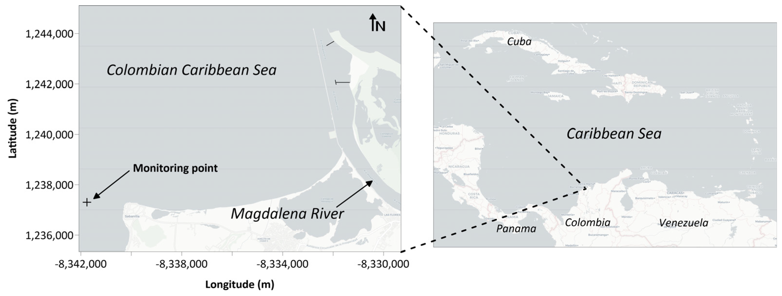
2. Materials and Methods
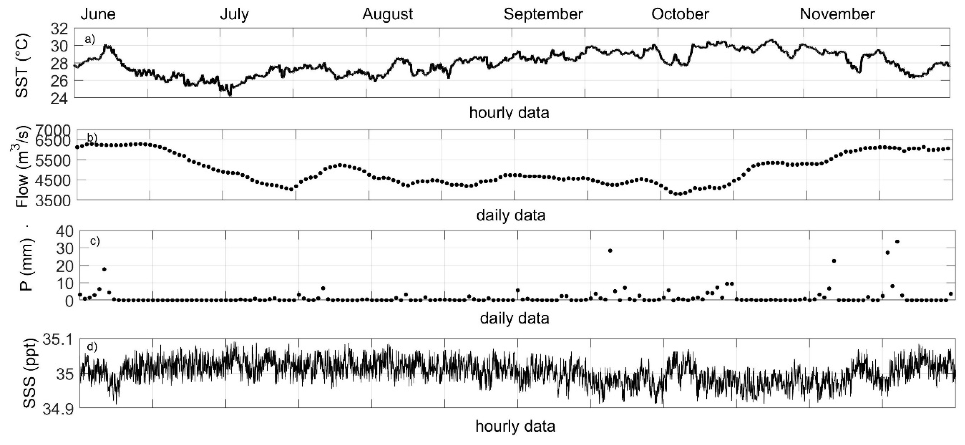
The study area was located in the Colombian Caribbean Sea, nearby the Magdalena River, Colombia’s largest and most important river (Figure 1).
The monitoring point is located at 11.038230° N 74.942785° W (8.9 m of water depth), and a 600 kHz ADCP with AST (Acoustic Surface Tracking) was deployed at the bottom to analyze the local and convective accelerations for six months. The accuracy of the water velocity measurements was ±1% of measured values (±0.5 cm/s), and the accuracy of AST parameters like the minimum footprint diameter, wavelength, and wave period was 0.4 m, 0.81 m and 0.93 s respectively, according to the technical recommendation of the ADCP manufacturer [27]. In this sense, the calculated wavelength of 35.76 m using the implicit equation of the dispersion relationship [28] indicated that the ADCP was located at intermediate waters and the wave data was recorded within the accuracy ranges of the instrument. The fluid acceleration was calculated using the derivative of the ADCP velocity records in respect to time δ U δ t . The measured parameters and recording configuration of ADCP are described in Table 1.
For identifying transient increments of current velocities in the monitoring point, the ADCP was placed 0.5 m above the bottom with 0.4 m of blanking distance and 0.4 m of window measurement to profile the water column up to the surface (y = 8 m). Also, the PUV (Pressure, U-V velocities) technique [29] was applied to estimate the wave energy spectrum, and the derived wave parameters as Significant Wave Height (Hs), Peak period (Tp), and direction. The WOA2018 database https://odv.awi.de/data/ocean/ (accessed on 1 April 2023) was used to retrieve information on the thermohaline properties of the study area, and climate data were obtained from the NCEP-North American Regional Reanalysis: NARR [30] to complement the analysis. To assess whether meso-scale atmospheric disturbances that occurred in the Caribbean Sea could have affected the local wind field of the study area (Figure 1), the met-ocean bulletins published by the Oceanographic and Hydrographic Research Center (CIOH, in Spanish) for the second semester of 2015 were read [31].
The dynamic properties of the water column were analyzed through the estimation of kinetic viscous properties of the hydrodynamic field, i.e., the Richardson number with the correction of mixing length by stratification, the turbulent kinetic energy through the Prandtl’s Mixing Length model, the vertical ( e v ) and horizontal eddy viscosity ( e h ) , and the vertical eddy diffusivity ( e h d ) ; details of mathematical formulae may be consulted in Deltares [32].
The Fast Fourier Transform was utilized to perform a time-frequency analysis to identify the oscillation modes of the current velocities and the variation of the wave energy spectrum during all six months. The wave parameters (Hs, Tp) were calculated through the spectral moment’s method mentioned by Holthuijsen [28]. Also, the Fourier analysis allowed verifying the quality of ADCP measurements by comparing the pressure spectral curves (PD) and wave orbital velocities records (u, v, w). An alternative way to identify whether the ADCP data are being properly recorded is inspecting the consistency of measurement frequency rate of the pressure and velocity sensors. To do this, a quality control of the ADCP records may be performed thorough a frequency domain analysis of data in spectral curves; then, the data would be considered well acquired when the more energetic pulses of the spectra have very similar natural periods.

3. Results

The inspection of quality data of ADCP records showed that PD and orbital wave velocities were in similar natural periods of main pulses (Figure 2), which evidenced the proper ADCP functioning. The energy density spectra showed periods between 2 and 12 s where they phase-matched within 6–10 s, but not for the lower periods (2–4 s), mainly because the high-frequency range is generated by nonlinear interactions such as breaking waves and triads, among others. It was observed that the three orbital wave velocities between 6 and 10 s showed synchronized periods and the same amplitudes, depicting circular trajectories of the wave profile, which suggests that the monitoring point was in the deep-water wave region, where the Airy Linear Theory is applicable; hence, the wave parameters depend on the period for developed sea-states [28]. The location of the monitoring point at the deep-water wave region not only guarantees that wave velocities are not perturbed by bottom friction or wave processes such as breaking, shoaling, reflection, or rip currents. To this end, further analysis of transient accelerations of current velocities will not be modified by the nonlinear wave processes mentioned above.

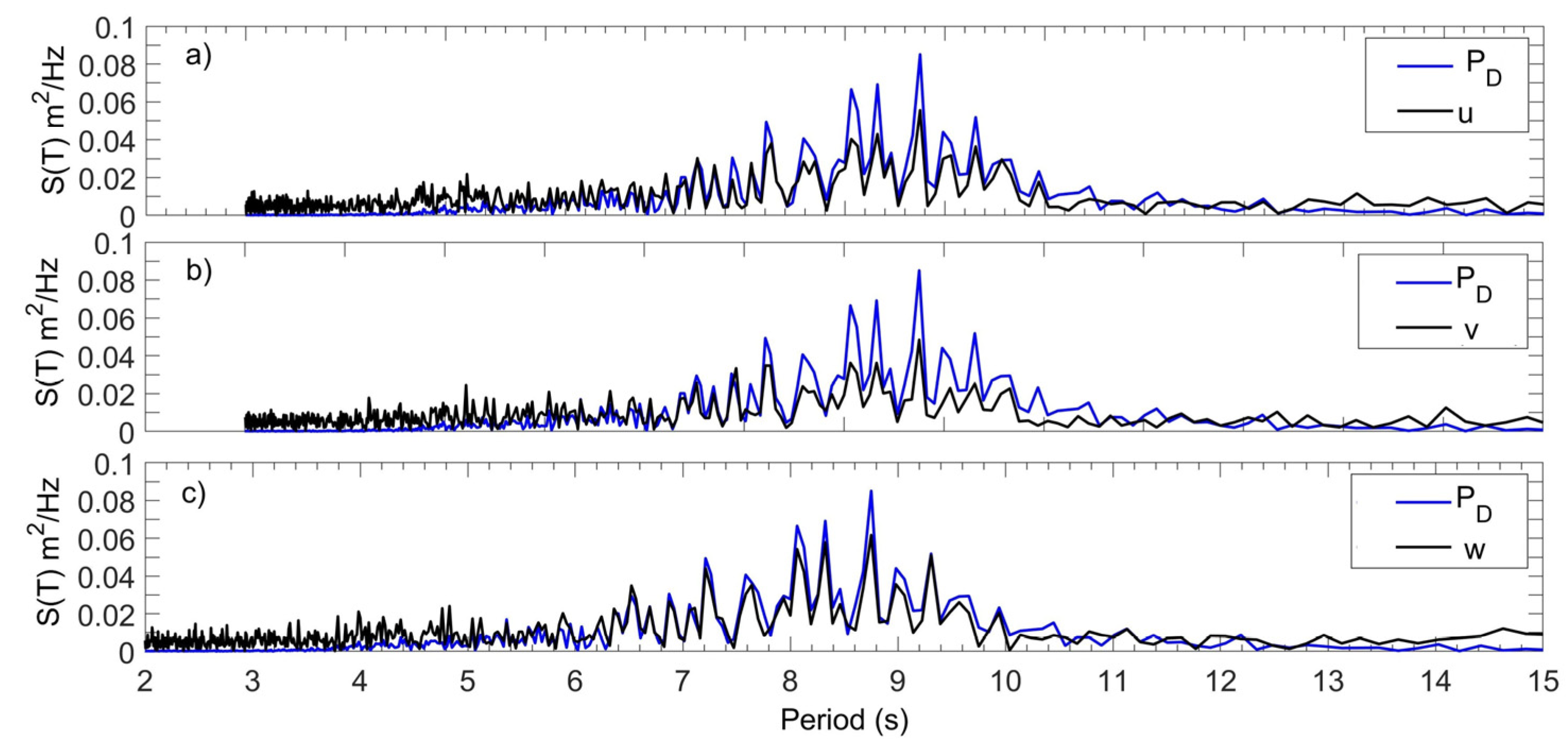
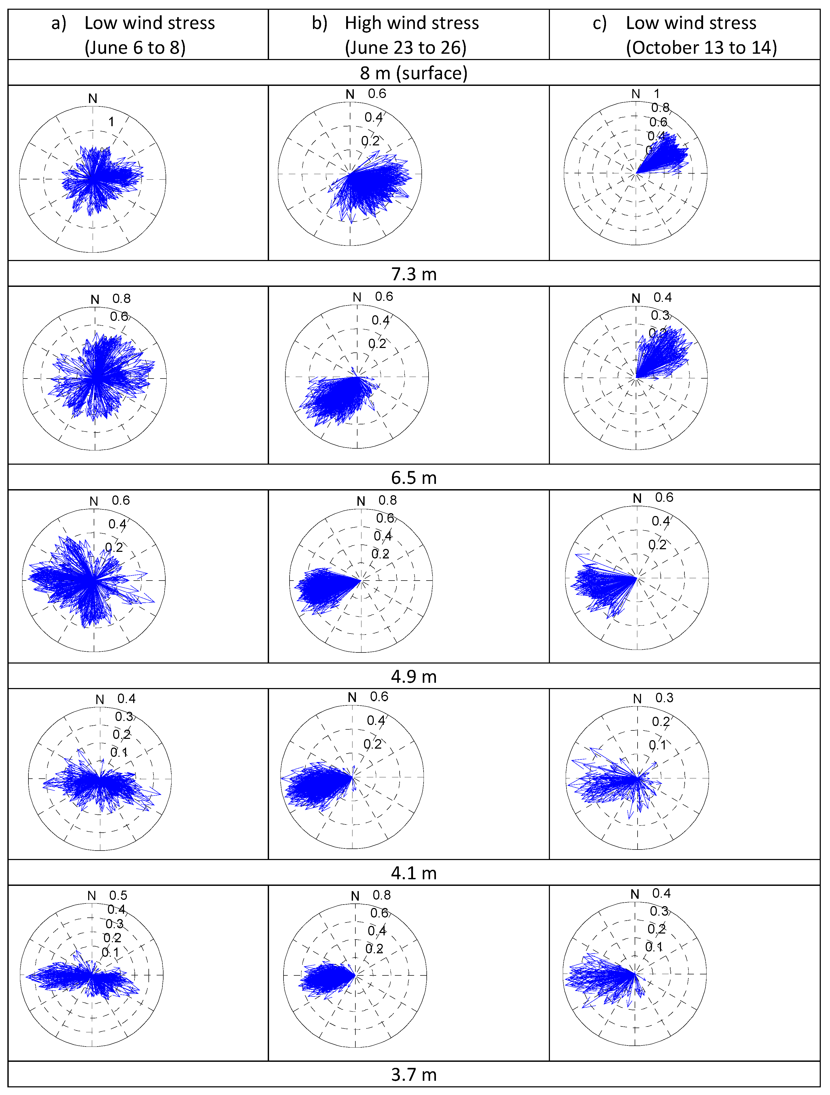
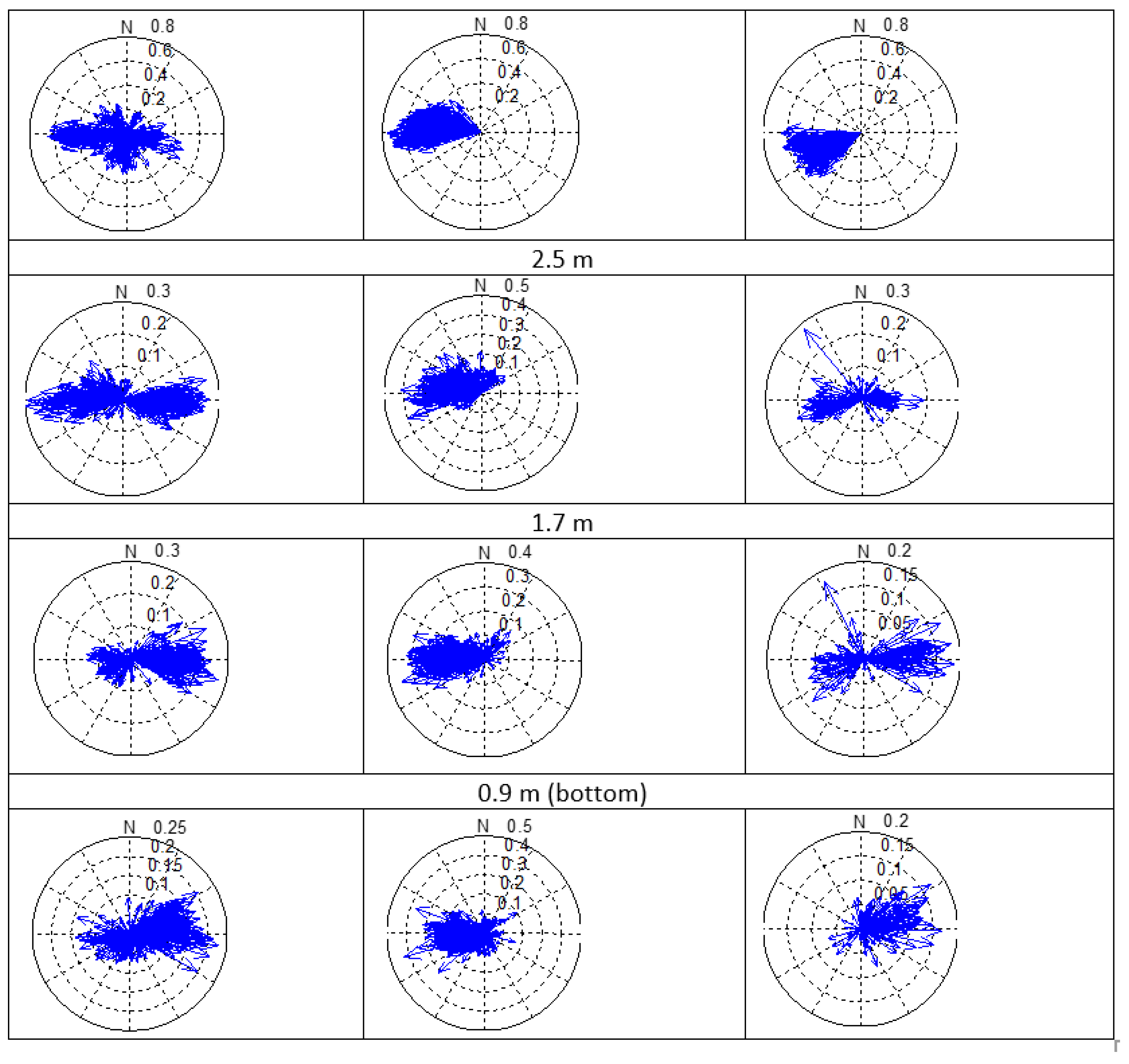
3.1. Time-Frequency Domain Analysis

After the quality inspection of ADCP records, a time-series analysis of climate parameters was conducted. In Figure 3, the sea surface temperature (SST) shows the lowest values in July and the highest in September and October. The river flow maximum values were about 6000 m3/s in June and November. High precipitation events were reported in June, October, and November. The sea surface salinity (SSS) depicted values between 34.9 ppt and 35 ppt in September, which were the lowest values, and July and November reported the highest values.
The maximum values of surface winds (Figure 4) were between 10 and 12 m/s (June to July) and lower velocities from the second half of September until November, with mean velocities of about 5 m/s. The predominance of winds was from 40° (north-east), with some changes from the south and south-west in most of the observed months. The precipitation and SST records (Figure 3) were associated with the wind records (Figure 4), because during the rainfall events, the wind velocities were under 5 m/s with low persistency from the 0° and 180°. In this sense, the decrement of wind surface stress over the water column generated an increment of the heat content that should be balanced with local evaporation processes. Hence, the reduction in wind speed allowed the generation of atmospheric convective processes that provoked the precipitations in the observed days.
These climate variables (see Figure 3 and Figure 4) correspond to the regular behavior of oceanographic and meteorological conditions of the region [8,33,34,35]. The variation of wave parameters during the studied period (Figure 5) pointed that maximum significant wave heights (Hs about 3 m) occurred from June to July, the lowest during September and October (0.2 m), with a Tp of 5 s and predominance to the south-west (220°). As expected, the wave parameters had correspondence with the wind behavior Figure 4, which means that the wind stress naturally controls the development of gravity waves.
The results of calculated wave spectra (Figure 6) showed that the highest energy density occurred in June and July and low energy densities occurred during September and October; hence, the wave spectra were controlled by the surface wind as was previously stated. The official bulletins of CIOH reported that several Caribbean Sea tropical waves occurred during the second semester of the year [36,37,38]. Accordingly, on June 4th of 2015, the first tropical wave arrived at the Colombian Caribbean Sea, impacting the region near the center area’s coastal zone where the monitoring point was located in this research (Figure 1). Hence, the tropical wave influenced the direction of local wind (100°) and waves (360°) (Figure 4 and Figure 5). Also, the wave spectra (Figure 6) reported low energy density during the event. Later, tropical waves affected the wind and wave directions from September to November as in June [39].

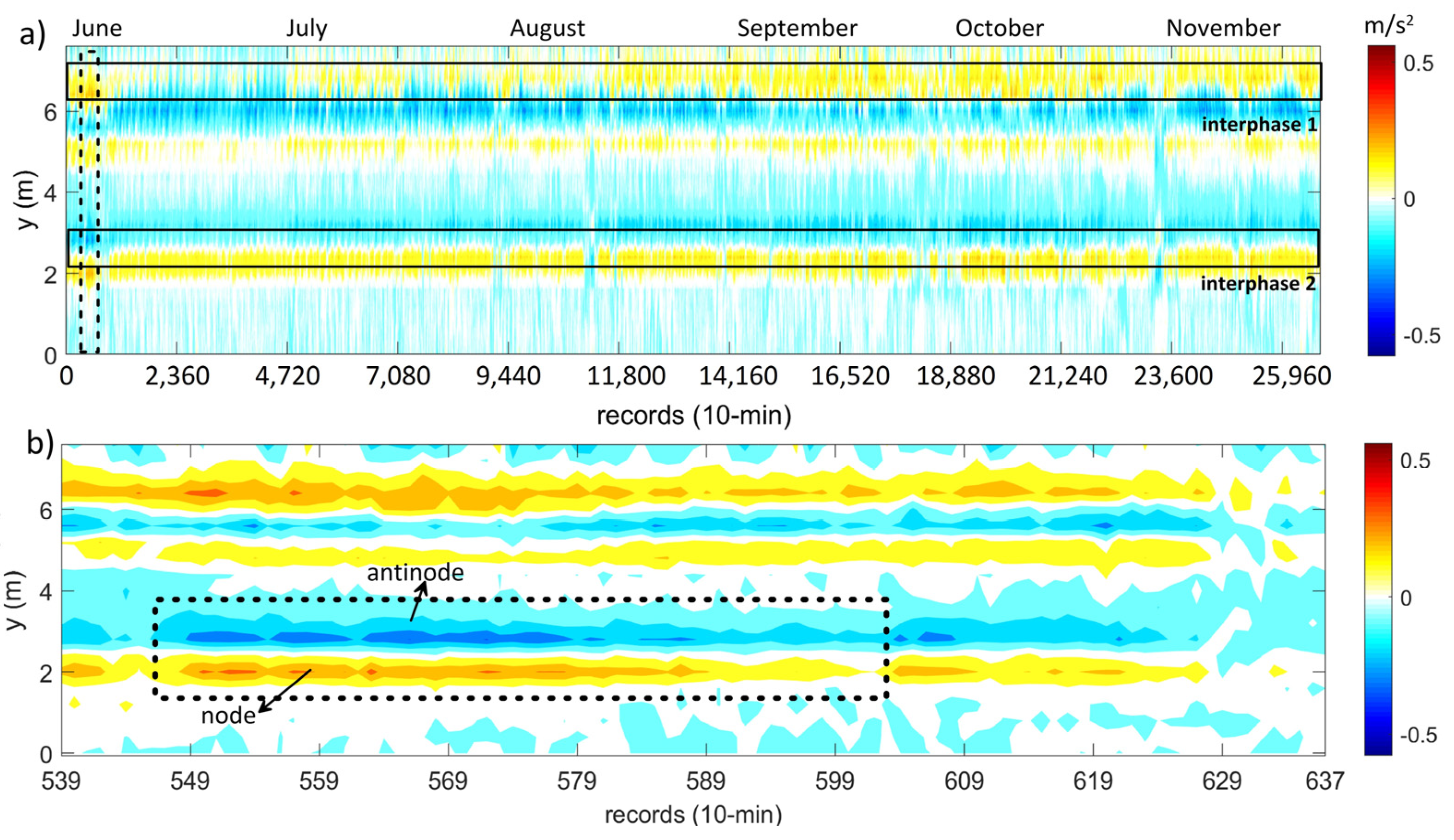
3.2. Transient Hydrodynamic Accelerations

The measured current velocities in the water column (Figure 7) showed a predominance to south-east direction (90–170°) in the surface layer (y = 7–8 m), and under this surface layer, the flow direction was to the south-west (220–260°). In the second week of June and September, the first and fourth week of October, maximum current velocities at the surface were between 0.60 m/s and 0.83 m/s, where the intensification of wind speed provoked the acceleration of surface currents (Figure 4 and Figure 7). Changes in the current profile were observed in October when the surface winds were the weakest. In these events at the surface layer, the flow direction was to the south-west (230–270°), and in deeper layers, the flow direction was to the east (90–110°), specifically ending July (one event), half of August (one event), six events in September, eight events in October and two events in November (Figure 7); the events occurred during low magnitude and high variability of surface winds (Figure 4).
The calculated current accelerations in Figure 8 evidenced the water energy conversion from kinetic to potential. In the first week of June, the wind speed was low and variable, wave heights were small, and the surface current velocities were about 0.8 m/s with positive accelerations. During the rest of July, the Ws increased almost without variability in the direction, which increased the wave heights, and a decrement of currents speed occurred, which evidenced the transfer of hydrokinetic energy to wave energy potential. In other words, the mean current velocity at surface layers was reduced because the wave heights increased due to the increment in Ws. After July, several episodes of acceleration and deceleration of surface currents occurred because of changes in Ws and Wd, allowing energy conversion between the hydrokinetic energy of currents and the potential energy of waves.
The acceleration profiles presented in Figure 8 depicted three acceleration levels (y = 2, 5 and 7 m) and three levels of deceleration (y = bottom, 3 m and 5.5 m). The acceleration at the surface layer was the most affected by wind stress, contrary to the deeper layers, where the measurements of acceleration and deceleration reported low fluctuations during the semester. Transient accelerations were observed from June to October mainly after a deceleration of currents; hence, to inspect these particular events, a zoom-in was generated in the first week of June (Figure 8b). The plot in Figure 8b showed maximum accelerations (0.5 m/s2) around 1 m below the surface (y = 7 m) and near the bottom (y = 2 m). These accelerations were followed by a deceleration of −0.5 m/s2; a transient wave was detected and highlighted by the dashed square. The acceleration corresponds to the wave node and the deceleration is the antinode; therefore, the in situ measurements allowed detecting a transient wave along the water column at the layer between 2 and 4 m.
A total of seven transient waves was observed during the semester, mainly in interphase 1, (y = 6.5–7.3 m) and in the layer close to the bottom (interphase 2) defined by y = 2.6–3.7 m. The wave node–antinodes (acceleration–deceleration of currents) showed a higher magnitude compared to interphase 2. These higher magnitudes of node–antinodes in the upper layer (interphase 1) were generated because interphase 2 (deeper layer) is denser as less affected by wind stress. This reduces the effect of wind stress in interphase 2; its higher density provoked a more symmetric shape of the transient wave in the time domain; ergo, the node–antinodes labeled in interphase 2 are more proportional compared to those of the upper ones of interphase 1 (Figure 8b).
The transient waves at lower layers of the water column were detected after a deceleration event at the surface layer because of the Ws decrement and reduction in wave heights: e.g., first week of June, third week of September and first week of October. To verify this assumption, the horizontal and vertical accelerations of one event of June and October were plotted (Figure 9 and Figure 10).
The variation of horizontal current acceleration–deceleration (ah) for both interphases 1 (y = 6.5–7.3 m) and 2 (y = 2.9–3.7 m) during the event of June (Figure 9) depicted the shape of six transient waves with ± 0.25 m/s2, with natural periods between 6 h, 12 h and 24 h. The vertical acceleration–deceleration (av) reported lower wave amplitudes not higher than ± 0.05 m/s2 at the upper layer (interphase 1), and the lower layer near to the bottom (interphase 2) showed lesser magnitudes but more harmonic with periods of about 12 h. In this sense, the event of June evidenced the predominance of horizontal transient accelerations of currents with three natural modes of oscillation compared to the vertical accelerations, suggesting that energy transfer was along the horizontal plane.
In the event of October (see Figure 10), it was possible to identify three transient waves in interphase 1 and 2 with similar magnitudes and periods ( ± 0.25 m/s2, 6 h, 12 h, 24, h) of horizontal acceleration–deceleration (ah). The vertical acceleration–deceleration (av) showed similar behavior in the lower layer (interphase 2) seen in the event of June (Figure 9).
To validate the magnitudes and natural periods of the identified transient waves in June and October, a spectral analysis of the acceleration records was performed (Figure 11). The root square to spectral density identified significant (most frequent) accelerations of 0.19 m/s2 and 0.16 m/s2 with periods of 23.87 h and 12.39 h, respectively. As a result, the periodogram agreed with the analysis of acceleration currents in the time domain (Figure 9 and Figure 10), confirming the presence of recurrent transient accelerations with semi- and daily periods.

4. Discussion

Dynamics of the Water Column

Figure 12 shows the ADCP current records for three events, two of them during low wind effect and the other with high wind effect. In the event of June 6 to 8, a low wind event (LWE) occurred provoking variable surface current vectors (Figure 12a). The lower layers evidenced the change in direction to 100° in June 8 (Figure 7, Figure 12) due to the wind weakening and its high variability occurred in the first week of June (Figure 4). In the second week of October, the wind decreased and reported winds from the south (180°), contrary to the recurrent north trade winds from the north-east (45°).
As a result, the water column in the event of October (Figure 12c) reported surface currents to the north-east (22.5–70°) because of the surface wind stress from the south. The wind stress effect fell from 8.5 m to the 7.5 m level; then, below this surface layer, the currents changed from south-west to south-east in the deeper layers (Figure 12c). In the June event, a high wind event (HWE) was reported (Figure 12b), the surface currents predominated to the southeast in the surface layer (y = 8.5 m). Below this level, the current predominated to the west along the water column. Comparing the event of HWE (Figure 12b) against the two events of the LWE (Figure 12a,c), this research evidenced that the weakening of north-trade winds and the increment of south-west winds allowed the currents headed to north-east (shore), mainly at the surface layer and at the bottom.
The identified TA in Figure 8 were analyzed for two events in June (Figure 9) and October (Figure 10), where LWEs were related to their generation. Considering that wind stress transfers energy to the water column in potential (wave heights) and kinetic (wave celerity, ocean currents) ways, it was necessary to analyze the stability of the water column in terms of viscous dynamic parameters for validating the effect of LWE and of HWE over the water column (Figure 12). As a result, viscous and turbulent parameters of the water column are plotted for two events with the presence of TA and one without TA (Figure 13).
The density profiles reported in June and October were similar, with slight differences at the surface and at the bottom. During the June events, the maximum wind speed decreases starting July. Due to the wind stress generated during June (Figure 4), the SST is the lowest of the second semester from the third week of June till the third week of July (Figure 3); the SSS did not report significant changes; then, upwelling–downwelling events were discarded. The higher density of July’s profile (1022.66 kg/m3) compared to those of June (1021.73 kg/m3) and October (1021.6 kg/m3) suggested that the lowest SST of July increased the water density, as seen in Figure 13. The horizontal currents of July were lower at the surface compared to those of June and October, so the LWE of July reduced the probability of high velocities and the occurrence of TA at the surface layer (Figure 7). The October profile showed the maximum current velocities at the surface (0.76 m/s, 70°) and a peak of 0.57 m/s headed to 265° at 2.8 m nearby to the bottom (Figure 13).
The Richardson number (Ri) from the surface to the level of 4.8 m (Figure 13) indicated that approximately the first 3 m of depth were sheared by winds, and turbulence was weakened by stable stratification. Below the 4.8 m level, Ri > 0.25; then, the high stability (laminar–not turbulent flow) in the lower layers did not report vertical mixing or strong inversion because of the dampened mechanical turbulence. The Turbulent Kinetic Energy (TKE) profile showed high values in interphase 1 (y = 6.5–7.3 m) and interphase 2 (y = 2.9–3.7 m) (Figure 13), where the highest values were reported in interphase 1 (4.6 m2/s2) for June, followed by October (1.784 m2/s2) and July (0.74 m2/s2). The TKE in interphase 2 was lower, with values for June, July and October of 1.4 m2/s2, 0.39 m2/s2 and 0.28 m2/s2, respectively. To this end, these results showed that the vortex intensified due to the presence of TA during the LWE, evidencing the propagation of TA along both interphases (Figure 10); hence, the lower the density, the higher the TKE and the TA in the hydrodynamic layer.
The horizontal and vertical eddy parameters (eh and ev) showed a higher vortex activity between interphases 1 and 2 (y = 3.6–4.8 m), where June and October reported the highest values of 0.04 m2/s and 0.25 m2/s, correspondingly. The aforementioned suggests that interphases 1 and 2 sheared between them and produced an intermediate layer with high elliptical vortex generation due to horizontal eddy viscosity (eh), which was six times higher than vertical eddy (ev) results. This intermediate layer reported maximum values of eddy diffusivity (evd) of 1.4 × 10⁻⁴ m2/s, which suggest that double-diffusive convection (DDC) occurred, like for the reported values in tropical waters in the Atlantic and Caribbean [40]. The DDC occurs in shallow regions [41], and the difficulty of measuring turbulent parameters through ADCP with long term- and high-interval resolution have limited the detection and understanding of DDC in the ocean [42]. In this sense, the methodology of this research may be applied in future studies for validating the presence of DDC in the Colombian Caribbean.
The Brunt–Väisälä frequency (N) pointed to the lower frequencies during the profile of June 8th and October 14th, which agreed with the low sea state reported on these dates. The July 1st profile reported the higher natural frequencies of the water column, evidencing more instability due to the higher wind effect and highest wave heights at the beginning of this month (Figure 4 and Figure 5).
The overall behavior of the current profile in the study area for the semester showed surface currents to the south-east (90–170°) with mean velocities of 0.5 m/s and a maximum of 0.8 m/s (Figure 7 and Figure 12). When surface winds decrease from August to November due to the weakening of the CLLJ [22,38,43,44,45], the Caribbean Counter Current (CCC) or the Panama-Colombia Counter current are affected, reducing its presence in the central coastal area (CCA) of the Colombian Caribbean [26]. When CCC turns back from the CCA to the north area of Colombian Caribbean, the Panama Colombia Counter Current (PCCC) [38] flows northmost near the Colombian coast carrying warm waters and forming a mixing zone when approaching the Magdalena River’s mouth [25]. Orfila et al. [26] reported spatial patterns of surface currents in the Colombian Caribbean Sea, where the hydrodynamic fields depicted a convergence zone near the coast (around the 11° N–75° W) due to the currents of PCCC heading north-east and the currents of the CCC flowing south-east.
The measured current velocities (Figure 7) showed a predominance to the east–south-east direction (90–135°) in the surface layer, and in the lower layers, a mean direction to west–south=west between 220 and 260° was observed. When winds changed in a couple of days to a recurrent direction coming from the north-east (0–45°) to the south (170°), the water column responded to that wind change and inverted the direction of its currents profile. As hypothesis, the modification of current profile when surface winds vary could be associated to a change in the interaction between the PCCC and the Magdalena River’s plume, which might be pointing to a convergence zone as seen in the currents field reported by Orfila et al. [26]; more in situ data such as satellite imagery and field campaigns would be needed for validation of this convergence area.
Latandret et al. [46] performed a tidal analysis in the Colombian Caribbean and pointed out that in the Puerto Velero tidal station, located 8 nautical miles to the south-west from the ADCP measurements of our research, the first three predominant tidal harmonics are K1, Sa and M2 respectively. The K1 and M2 harmonics identified in the study have 23.93 h and 12.42 h of period; hence, the semi- and daily periods of the transient accelerations observed in the time (Figure 9 and Figure 10) and frequency domain (Figure 11) might be controlled by these tidal constituents. In this sense, when surface winds reduce the wind stress on the water column in the couple of days as was argued in the above paragraph, not only the current profile changes, but also the K1 and M2 tidal harmonics intensify its effect on the hydrodynamics, provoking the generation of the transient acceleration along the water column. This hypothesis must be validated with further nonlinear analysis performed in the study area [47] using new ADCP current profiles, water level records and surface wind measurements.

5. Conclusions

This work deployed an ADCP profiler in shallow waters of the Colombian Caribbean coast for six months, measuring at high time intervals (10–17 min). The analysis of marine currents, wave parameters and climate variables of the study area allowed to reach the following statements. The hydrodynamics of the study area showed three layers according to the kinetic and turbulent–viscous results of ADCP profiles. The surface layer is dominated by north trade winds, and during the second semester, south-west wind affects the local hydrodynamics. When north trade winds predominate due to the effect of the Caribbean Low-Level Jet, the Caribbean Counter Current (CCC) intensifies and flows southernmost, carrying lower and denser waters to the study area and generating a current profile with currents to the south-east at the surface (maximum of 0.8 m/s) and to the south-west in the lower layers (0.1–0.5 m/s).
In this sense, in the study area the presence of a convergence zone generated by the CCC and PCCC, a controlled area by the CLLJ, is possible. It is likely that when the north trade winds decrease, the intermittent incursion of PCCC at the study area eases and transient waves propagating along the horizontal plane are provoked. These transient waves intermittently modify the water column’s kinetic energy during 6 h and 24 h. According to the kinetic and viscous–turbulent parameters of the measured water column, it is possible that in this convergence zone, the DDC processes occurs around 4 m of depth (mid-layer) with eddy diffusivity (evd) of 1.4 × 10⁴ m2/s.
This research is the first of its kind that evidenced the presence of transient waves in the Colombian Caribbean, which occurred due to variations of surface winds during short-term events (days < 3). These internal waves with maximum magnitudes and natural periods of ± 0.25 m/s2, 6 h, 12 h, 24, h, respectively, propagated in two specific water depths, one located in the deepest layer between y = 3.7 and 2.9 m from the bottom, and the second near to the surface (7.3–6.5 m). Hence, this research evidenced the presence of transient currents that might affect the power generation and structural health of marine technology of future marine energy plants in Colombia.
For future research, it is recommended to measure currents, waves and thermohaline parameters for more than 1 year, with high time intervals (less than 10 min), to widen the understanding of hydrodynamics at the study area and validate the presence of tropical DDC. Also, imagery satellite analysis might provide more information that could validate the hypothesis of presence of a convergence zone in the study area, and new current profiles, water level and winds measurements are recommended to validate the effect of K1 and M2 tidal constituents.

Author Contributions

Conceptualization, J.G.R.-B.; methodology, J.G.R.-B.; validation, J.G.R.-B.; J.G.R.-B.; investigation J.G.R.-B.; resources, J.G.R.-B.; writing—original draft preparation, J.G.R.-B.; writing—review and editing, J.G.R.-B., J.J.C.E., A.L.C.-L., A.G. and J.L.G.V.; visualization, J.G.R.-B.; supervision, J.G.R.-B.; project administration, J.G.R.-B.; funding acquisition, J.G.R.-B. All authors have read and agreed to the published version of the manuscript.

Funding

This research was funded by Universidad del Norte, grant number [2013–2017 (2013–2017)], and Universidad del Valle and “The APC was funded by Universidad del Valle through the research project C.I 1214”.

Data Availability Statement

The measured oceanographic data were provided by the research institute IDEHA of Universidad del Norte.

Acknowledgments

First author acknowledges IDEHA, Universidad del Norte and Universidad del Valle for supporting the research.

Conflicts of Interest

The authors declare no conflict of interest.

List of Symbols and Abbreviatures

ahHorizontal acceleration (m/s2)
avVertical acceleration (m/s2)
Hs.Wave height (m)
TpPeak period (s)
u, v, wWave orbital velocities (m/s)
SSTSea surface temperature (°C)
SSSSea surface salinity (ppt)
PDaily accumulated precipitation (mm)
WsWind speed (m/s)
WdWind direction (°)
SSTSea Surface Temperature (°C)
rhoWater density (kg/m3)
RiRichardson number
TKETurbulent kinetic energy (m2/s2)
ADCPAcoustic Doppler Current profiler
ASTAcoustic Surface Tracking
CLLJCaribbean Low-Level Jet winds
CCCCounter Caribbean Current
CIOHOceanographic and Hydrographic Research Center
DDCDouble-diffusive convection
PCCCPanama Colombia Counter Current
NARRNCEP-North American Regional Reanalysis database
PDPressure spectral curves
u, vHorizontal velocity components
UHorizontal velocity resultant
LWELow wind event
HWEHigh wind event

References

  1. Stephens, S.A.; Ramsay, D.L. Extreme Cyclone Wave Climate in the Southwest Pacific Ocean: Influence of the El Niño Southern Oscillation and Projected Climate Change. Glob. Planet. Chang. 2014, 123, 13–26. [Google Scholar] [CrossRef] [Green Version]
  2. Roy, B.; Penha-Lopes, G.P.; Uddin, M.S.; Kabir, M.H.; Lourenço, T.C.; Torrejano, A. Sea Level Rise Induced Impacts on Coastal Areas of Bangladesh and Local-Led Community-Based Adaptation. Int. J. Disaster Risk Reduct. 2022, 73, 102905. [Google Scholar] [CrossRef]
  3. Hendrix, C.S.; Glaser, S.M.; Lambert, J.E.; Roberts, P.M. Global Climate, El Niño, and Militarized Fisheries Disputes in the East and South China Seas. Mar. Policy 2022, 143, 105137. [Google Scholar] [CrossRef]
  4. Xu, H.; Zhuang, C.C.; Guan, X.; He, X.; Wang, T.; Wu, R.; Zhang, Q.; Huang, W. Associations of Climate Variability Driven by El Niño-Southern Oscillation with Excess Mortality and Related Medical Costs in Chinese Elderly. Sci. Total Environ. 2022, 851, 158196. [Google Scholar] [CrossRef]
  5. Paz, S.; Semenza, J.C. El Niño and Climate Change—Contributing Factors in the Dispersal of Zika Virus in the Americas? Lancet 2016, 387, 745. [Google Scholar] [CrossRef] [Green Version]
  6. Rueda-Bayona, J.G.; Guzmán, A.; Eras, J.J.C.; Silva-Casarín, R.; Bastidas-Arteaga, E.; Horrillo-Caraballo, J. Renewables Energies in Colombia and the Opportunity for the Offshore Wind Technology. J. Clean. Prod. 2019, 220, 529–543. [Google Scholar] [CrossRef]
  7. Gato, L.M.C.; Henriques, J.C.C.; Carrelhas, A.A.D. Sea Trial Results of the Biradial and Wells Turbines at Mutriku Wave Power Plant. Energy Convers. Manag. 2022, 268, 115936. [Google Scholar] [CrossRef]
  8. Rueda-Bayona, J.G.; Guzmán, A.; Cabello Eras, J.J. Selection of JONSWAP Spectra Parameters during Water-Depth and Sea-State Transitions. J. Waterw. Port Coast. Ocean Eng. 2020, 146, 04020038. [Google Scholar] [CrossRef]
  9. Rueda-Bayona, J.G.; Osorio-Arias, A.; Guzmán, A.; Rivillas-Ospina, G. Alternative Method to Determine Extreme Hydrodynamic Forces with Data Limitations for Offshore Engineering. J. Waterw. Port Coast. Ocean Eng. 2018, 145, 16. [Google Scholar] [CrossRef]
  10. Rueda-Bayona, J.G.; Gil, L.; Calderón, J.M. CFD-FEM Modeling of a Floating Foundation under Extreme Hydrodynamic Forces Generated by Low Sea States. Math. Model. Eng. Probl. 2021, 8, 888–896. [Google Scholar] [CrossRef]
  11. Pichault, M.; Vincent, C.; Skidmore, G.; Monty, J. LiDAR-Based Detection of Wind Gusts: An Experimental Study of Gust Propagation Speed and Impact on Wind Power Ramps. J. Wind Eng. Ind. Aerodyn. 2022, 220, 104864. [Google Scholar] [CrossRef]
  12. Tan, K.; Islam, S. Optimum Control Strategies in Energy Conversion of PMSG Wind Turbine System without Mechanical Sensors. IEEE Trans. Energy Convers. 2004, 19, 392–399. [Google Scholar] [CrossRef]
  13. Xie, T.; Wang, T.; He, Q.; Diallo, D.; Claramunt, C. A Review of Current Issues of Marine Current Turbine Blade Fault Detection. Ocean Eng. 2020, 218, 108194. [Google Scholar] [CrossRef]
  14. Rueda-Bayona, J.G.; Paez, N.; Eras, J.J.C.; Gutiérrez, A.S. DOE-ANOVA to optimize hydrokinetic turbines for low velocity conditions. Math. Model. Eng. Probl. 2022, 9, 979–988. [Google Scholar] [CrossRef]
  15. Li, Y.; Wang, C.; Liang, C.; Li, J.; Liu, W. A Simple Early Warning Method for Large Internal Solitary Waves in the Northern South China Sea. Appl. Ocean Res. 2016, 61, 167–174. [Google Scholar] [CrossRef]
  16. Sato, M.; Klymak, J.M.; Kunze, E.; Dewey, R.; Dower, J.F. Turbulence and Internal Waves in Patricia Bay, Saanich Inlet, British Columbia. Cont. Shelf Res. 2014, 85, 153–167. [Google Scholar] [CrossRef]
  17. Haibin, L.; Xie, J.; Xu, J.; Chen, Z.; Liu, T.; Cai, S. Force and Torque Exerted by Internal Solitary Waves in Background Parabolic Current on Cylindrical Tendon Leg by Numerical Simulation. Ocean Eng. 2016, 114, 250–258. [Google Scholar] [CrossRef]
  18. Chen, M.; Chen, K.; You, Y.X. Experimental Investigation of Internal Solitary Wave Forces on a Semi-Submersible. Ocean Eng. 2017, 141, 205–214. [Google Scholar] [CrossRef]
  19. Bastidas-Salamanca, M.; Gabriel Rueda-Bayona, J. Pre-Feasibility Assessment for Identifying Locations of New Offshore Wind Projects in the Colombian Caribbean. Int. J. Sustain. Energy Plan. Manag. 2021, 32, 139–154. [Google Scholar] [CrossRef]
  20. Ortega, S.; Osorio, A.F.; Agudelo, P. Estimation of the Wave Power Resource in the Caribbean Sea in Areas with Scarce Instrumentation. Case Study: Isla Fuerte, Colombia. Renew. Energy 2013, 57, 240–248. [Google Scholar] [CrossRef]
  21. Orejarena-Rondón, A.F.; Restrepo, J.C.; Correa-Metrio, A.; Orfila, A. Wave Energy Flux in the Caribbean Sea: Trends and Variability. Renew. Energy 2022, 181, 616–629. [Google Scholar] [CrossRef]
  22. Bastidas-Salamanca, M.; Rueda-Bayona, J.G. Effect of Climate Variability Events over the Colombian Caribbean Offshore Wind Resource. Water 2021, 13, 3150. [Google Scholar] [CrossRef]
  23. Osorio, A.F.; Ortega, S.; Arango-Aramburo, S. Assessment of the Marine Power Potential in Colombia. Renew. Sustain. Energy Rev. 2016, 53, 966–977. [Google Scholar] [CrossRef]
  24. Andrade, C.A.; Barton, E.D.; Mooers, C.N.K. Evidence for an Eastward Flow along the Central and South American Caribbean Coast. J. Geophys. Res. Ocean. 2003, 108, 16. [Google Scholar] [CrossRef] [Green Version]
  25. Fernando Pareja Román, L.; Cristina Díaz Guevara, D.; Tatiana Rodríguez Tobar, Á.; Liliana Villegas Bolaños, N.; Ernesto Pérez Santos, I.; Pérez, N. Análisis Del Transporte y Bombeo de Ekman En El Caribe Colombiano Entre 1999 y 2009. Bol. Cient. CIOH 2013, 31, 3–12. [Google Scholar] [CrossRef]
  26. Orfila, A.; Urbano-Latorre, C.P.; Sayol, J.M.; Gonzalez-Montes, S.; Caceres-Euse, A.; Hernández-Carrasco, I.; Muñoz, Á.G. On the Impact of the Caribbean Counter Current in the Guajira Upwelling System. Front. Mar. Sci. 2021, 8, 128. [Google Scholar] [CrossRef]
  27. NORTEK. The Comprehensive Manual–ADCP. Available online: https://www.nortekgroup.com/fr/products/awac-600-khz/pdf (accessed on 11 July 2023).
  28. Holthuijsen, L.H. Waves in Oceanic and Coastal Waters; Cambridge University Press: Cambridge, MA, USA, 2007; ISBN 978-0-51-161853-6. [Google Scholar]
  29. NORTEK. Ocean Waves. Available online: https://www.nortekgroup.com/products/awac-600-khz (accessed on 27 July 2023).
  30. NOAA NCEP. North American Regional Reanalysis: NARR. Available online: https://psl.noaa.gov/data/gridded/data.narr.html (accessed on 27 July 2023).
  31. DIMAR-CIOH. CIOH. Climatología de Los Principales Puertos Del Caribe Colombiano-Barranquilla; Dirección General Marítima: Cartageina de Indias, Colombia, 2010; Available online: https://www.cioh.org.co/index.php/en/areas-del-conocimiento/sm-oceanografia-operacional/productos-y-servicios-arope/climatologia-puertos-caribe-colombiano (accessed on 1 May 2023).
  32. Deltares Delft3D-FLOW. Simulation of Multi-Dimensional Hydrodynamic Flows and Transport Phenomena, Including Sediments–User Manual. 2014. Available online: https://usermanual.wiki/Pdf/Delft3DFLOWUserManual.885467064/help (accessed on 27 July 2023).
  33. Bastidas Salamanca, M.L.; Figueroa Casas, A. Seguimiento Satelital de Las Condiciones Océano-Atmosféricas Asociadas a Los Eventos de Precipitación En Colombia Durante El Evento La Niña 2010–2011. Bol. Cient. CIOH 2014, 32, 123–134. [Google Scholar] [CrossRef]
  34. Andrade, C. Análisis de La Velocidad Del Viento En El Mar Caribe. Bol. Cient. CIOH 1993, 15, 33–43. [Google Scholar] [CrossRef]
  35. Wang, C.; Lee, S.K. Atlantic Warm Pool, Caribbean Low-Level Jet, and Their Potential Impact on Atlantic Hurricanes. Geophys. Res. Lett. 2007, 34. [Google Scholar] [CrossRef] [Green Version]
  36. Amador, J.A.; Alfaro, E.J.; Lizano, O.G.; Magaña, V.O. Atmospheric Forcing of the Eastern Tropical Pacific: A Review. Prog. Oceanogr. 2006, 69, 101–142. [Google Scholar] [CrossRef]
  37. Amador, J.A. The Intra-Americas Sea Low-Level Jet: Overview and Future Research. Ann. N. Y. Acad. Sci. 2008, 1146, 153–188. [Google Scholar] [CrossRef] [PubMed] [Green Version]
  38. Wang, C. Variability of the Caribbean Low-Level Jet and Its Relations to Climate. Clim. Dyn. 2007, 29, 411–422. [Google Scholar] [CrossRef] [Green Version]
  39. DIMAR-CIOH. Pronóstico Climático Del Caribe Colombiano Junio 2015; Dirección General Marítima: Cartagena de Indias, Colombia, 2015. [Google Scholar] [CrossRef] [Green Version]
  40. Schmitt, R.W.; Ledwell, J.R.; Montgomery, E.T.; Polzin, K.L.; Toole, J.M. Enhanced Diapycnal Mixing by Salt Fingers in the Thermocline of the Tropical Atlantic. Science 2005, 308, 685–688. [Google Scholar] [CrossRef] [PubMed]
  41. Hirano, D.; Kitade, Y.; Nagashima, H.; Matsuyama, M. Characteristics of Observed Turbulent Mixing across the Antarctic Slope Front at 140°E, East Antarctica. J. Oceanogr. 2010, 66, 95–104. [Google Scholar] [CrossRef]
  42. Nakano, H.; Yoshida, J. A Note on Estimating Eddy Diffusivity for Oceanic Double-Diffusive Convection. J. Oceanogr. 2019, 75, 375–393. [Google Scholar] [CrossRef] [Green Version]
  43. Muñoz, E.; Busalacchi, A.J.; Nigam, S.; Ruiz-Barradas, A. Winter and Summer Structure of the Caribbean Low-Level Jet. J. Clim. 2008, 21, 1260–1276. [Google Scholar] [CrossRef] [Green Version]
  44. Whyte, F.S.; Taylor, M.A.; Stephenson, T.S.; Campbell, J.D. Features of the Caribbean Low Level Jet. Int. J. Climatol. 2008, 28, 119–128. [Google Scholar] [CrossRef]
  45. Villegas, N.; Malikov, I.; Farneti, R. Sea Surface Temperature in Continental and Insular Coastal Colombian Waters: Observations of the Recent Past and near-Term Numerical Projections. Lat. Am. J. Aquat. Res. 2021, 49, 307–328. [Google Scholar] [CrossRef]
  46. Latandret-Solana, S.A.; Torres Parra, R.R.; Herrera Moyano, D.P. Ocean Tides in the Colombian Basin and Atmospheric Contribution to S2. Dyn. Atmos. Ocean. 2023, 102, 101356. [Google Scholar] [CrossRef]
  47. Rueda-Bayona, J.G.; Carrillo, J.; Cabello Eras, J.J. The Wind-Current-Water Levels Effect over Surface Wave Parameters Nearby the Magdalena River Delta: A Numerical Approach. Math. Model. Eng. Probl. 2023, 10, 993–1002. [Google Scholar] [CrossRef]
Figure 1. Location of the monitoring point. Coordinates in Magna Sirgas unit system.
Water 15 02725 g001
Figure 2. Comparison of pressure (PD) vs. orbital wave velocities (a) u, (b) v, (c) w at first window measurement (bottom) recorded by the ADCP.
Water 15 02725 g002
Figure 3. Time-series of (a) SST, (b) river flow, (c) daily accumulated precipitation (P), and (d) SSS for June 3rd to December 1st of 2015.
Water 15 02725 g003
Figure 4. Time-series of the local surface wind for June 3rd to December 1st of 2015. Ws: Wind speed, Wd: Wind direction.
Water 15 02725 g004
Figure 5. Wave parameters for June 3rd to December 1st of 2015.
Water 15 02725 g005
Figure 6. Hourly energy (E) wave spectra for June 3rd to December 1st of 2015.
Water 15 02725 g006
Figure 7. Mean hourly current parameters measured by the ADCP for June 3rd to December 1st of 2015, u and v are horizontal velocity components.
Water 15 02725 g007
Figure 8. Horizontal current acceleration calculated from ADCP records: (a) June 3rd to December 1st of 2015. (b) Zoom-in at second week of June.
Water 15 02725 g008
Figure 9. Horizontal (ah) and vertical (av) components of acceleration for currents calculated from ADCP records with 10 min intervals for the period June 6th 06:00 h to 8th 07:00 of 2015.
Water 15 02725 g009
Figure 10. Horizontal (ah) and vertical (av) components of acceleration for currents calculated from ADCP records with 10 min intervals for October 13th 20:40 h to 14th 18:20 of 2015.
Water 15 02725 g010
Figure 11. Periodogram of horizontal (ah) accelerations calculated from ADCP records with 10 min intervals from June 3rd to December 1st of 2015.
Water 15 02725 g011
Figure 12. Current vectors with 10 min time intervals distributed along the water column for three events during 2015: (a) June 6 to 8, (b) June 23 to 26, (c) October 13 to 14.
Water 15 02725 g012aWater 15 02725 g012b
Figure 13. Dynamic and kinetic energy properties of current profiles for 3 events during June 8th (TA event), July 1st and October 14th (TA event) of 2015.
Water 15 02725 g013
Table 1. Measurement characteristics of the deployed ADCP.
ParameterElapsed Time (dd-mm-yyyy-hh)Time Interval (h)Duration of Each Measurement Event (min)Measurement Frequency of Each Event (Hz).
Hydrostatic pressure at bottom (dbar) 03-06-2015-
12 to 11-12-
2015-18
1 10 1
3D Orbital wave velocities (m/s)03-06-2015-
12 to 11-12-
2015-18
1 17 2
Free surface (m)03-06-2015-
12 to 11-12-
2015-18
1 17 2
Temperature (°C) 03-06-2015-
12 to 11-12-
2015-18
1 17 2
Horizontal current velocity (m/s)03-06-2015-
12 to 11-12-
2015-18
1 10 1
Disclaimer/Publisher’s Note: The statements, opinions and data contained in all publications are solely those of the individual author(s) and contributor(s) and not of MDPI and/or the editor(s). MDPI and/or the editor(s) disclaim responsibility for any injury to people or property resulting from any ideas, methods, instructions or products referred to in the content.

