Three-Dimensional Smooth Particle Hydrodynamics Modelling of Liquid–Sediment Interaction at Coastline Region

Abstract

The three-dimensional liquid–sediment system of a coastline was investigated using experimental and numerical approaches. A scaled-down model of the coastline was numerically studied using smooth particle hydrodynamics (SPH). The flow dynamics and the impacts of the wave frequency and the seaward slope angle on the breaking wave characteristics of the two-phase liquid–sediment interaction were parametrically studied. A particle image velocimetry (PIV) experiment was conducted to validate the SPH predictions. It was found that the flow profiles obtained by the PIV and SPH are in good agreement both qualitatively and quantitatively. The maximum velocity of the fluid flow was recorded as 0.5623 m/s in the SPH simulation, but as 0.5860 m/s in the PIV experimental, with a percentage difference of 4.21%. Subsequently, it was found that the breaking wave characteristic is surging at the wave frequency range of $f<0.15$ Hz, plunging at $0.15<f<0.55$ Hz, and spilling at $0.55<f\le 1.0$ Hz. It was also established that at a particular Froude number, it is observed that spilling, plunging, and surging wave breakers are produced at low, mid, and high seaward slope angles, respectively. Meanwhile, increasing the Froude number increases the tendency to produce spilling or plugging breaking waves, irrespective of the slope angle. Ultimately, this study has demonstrated the presented methodology’s usefulness in investigating coastlines’ liquid–sediment interaction properties.

1. Introduction

Developmental constructions are mainly situated around the coastal areas for different purposes, such as tourism and power generation. A power plant is built near a coastline to continuously use seawater as a cooling fluid while simultaneously generating electricity. However, if not mitigated, coastal erosion due to sediment transport by the sea wave harms the power plant and other constructions near the coastline. Hence, establishing the dynamics of the liquid and sediment interaction due to the impulse of the sea wave is pertinent to mitigating the damaging impact of sediment erosion. This study investigates the liquid–sediment interaction of a coastline near the Tenaga Nasional Berhad (TNB) Tuanku Jaafar power plant in Malaysia to establish the interaction’s impact on the TNB power plant.

Biological activities, such as waves, tides, groundwater, and storm surges, form a coastline. The main hydrodynamic forces, such as currents and waves, can cause sediment transport such that the sandy beaches accrete and erode due to continuous changes in wave conditions over the years [1]. The sediment erosion occurs due to the induced shearing forces imposed by rapid fluid flow at the surface of the sediment [2]. Powerful waves can push and hit the surrounding land due to numerous contacts, creating new landforms after carving out the area [3,4]. Soil erosion is caused by the direct dynamic force of the wind, whereby wind actions such as whirlwinds, hurricanes, and tornadoes can move the weathered material [5]. One factor that makes wind an erosion agent at coastlines is the presence of materials such as sand and dust, which are easily transported during wind flow.

Compared to experiments, numerical approaches have been extensively applied to problems in fluid mechanics due to their cost, time-saving prospects, and safety concerns [6]. The classical simulation techniques of using the traditional mesh-based Eulerian method are challenging to model the non-Newtonian fluid interaction with sediment compared to the Lagrangian method. Therefore, a Smooth Particle Hydrodynamics (SPH) approach [7,8], which is based on the Lagrangian method, is known to have good capabilities in solving problems of the interactions between sand particles (sediment) and the rapidly moving sea waves [9].

SPH has been widely applied to simulate liquid–sediment interaction in various engineering systems. For instance, Maeda et al. [10] developed a two-dimensional (2D) SPH model for multi-phase interaction occurring from the contact of sea waves and sand particles. The developed model combines discrete and continuum analyses in the interaction among sediment, liquid, and air phases. The SPH model is extended in [11] to study the noncohesive sediment flushing induced by a rapid fluid flow in a 2D water–sediment system of an artificial reservoir. Based on the Mohr–Coulomb yielding criterion and Shields theory, the study defined liquid and sediment materials as weakly compressible viscous fluids. The method is also applied in [12] to develop a multi-physics model for fluid–structure–sediment interactions in a 2D marine system, which is difficult to study through the traditional mesh-based Lagrangian solver. Shi et al. [13] developed a two-phase sediment transport SPH model using large eddy simulation to model the turbulence effect of the sea wave and a modified Smagorinsky model to account for the influence of sediment particles on wave turbulence. The developed approach models the water as a weakly compressible fluid and the sediment as an incompressible fluid. An incompressible SPH scheme that incorporates an improvement in the solution of multi-phase, non-Newtonian, and turbulence flows to model landslides in a 2D fluid flow system is presented in [14]. In similar research, Tan and Chen [15] applied a hybrid discrete element method (DEM) with SPH to model deformable landslides. Although the SPH method has been successfully used to study different practical liquid–sediment interaction problems, its main drawback is that it requires substantial computational resources, such as hardware acceleration and parallel computing, which are expensive to buy and maintain. An open-source DualSPHysics SPH solver is developed in [16] to enhance the performance of the SPH solver by parallelizing the solver on graphics processing units (GPUs). It is established that GPUs are a cheaper alternative to supercomputers for accelerating the SPH model. The performance enhancement of the SPH solver is extended in [2] to a 3D model, which requires a more significant number of particles, by coupling the DualSPHysics code with a non-Newtonian Herschel–Bulkley–Papanastasiou sediment formulation. The coupling is successfully implemented as it achieves a computational speed of 58 times faster compared to an optimized single-threaded serial code. The performance of the SPH model has also been enhanced by the development of a modified scheme [17] that combines the SPH method with a numerical wave flume, resulting in higher computational efficiency than the conventional SPH.

Particle image velocimetry (PIV) is an optical method of flow visualization that has been widely applied to acquire instantaneous velocity measurements and related properties of fluids [18]. The work of Abas et al. [19] demonstrated the capabilities of PIV in capturing flow visualization. Similarly, the study involving large-scale particle image velocimetry (LSPIV) was presented in [20] to evaluate the flow pattern. Furthermore, Azman et al. [21] also showed the capabilities of PIV to compute flow patterns, velocity, and aeration efficiency. In addition, Peltier et al. [22] found that relative flow velocity is slightly higher when using LSPIV than conventional PIV. Meanwhile, Leuptow et al. [23] analyzed PIV for granular flows, which is relatively easy to measure particle displacement or velocities at clear side walls.

Based on the current literature, there is a lack of research conducted on complex coastal areas to analyze sediment transport using SPH. A limited number of research works also exist on investigating the interactions between sea waves and sediment and the impact of the interaction on deposition and erosion at the coastline area. Most of the past research on the topic has been limited to the 2D liquid–sediment model, and the incorporation of GPUs in the SPH solver is still limited. To address the cited limitations, the current work attempts to create a GPU-incorporated three-dimensional SPH model for a coastal liquid–sediment interaction with minimal computational effort. Sediment transport during the interaction is the central focus of this study. A PIV experimental set-up was also developed to measure the liquid–sediment interaction phenomenon of the coastal system.

2. Materials and Methods

2.1. Data Collection and Analysis

Relevant data, such as sand and sea wave velocity, frequency, and amplitude, are collected from the study site at a coastal area near the Tuanku Jaafar power station at Port Dickson, Negeri Sembilan. These data are used as raw data and materials (such as sand) to develop a simplified liquid–sediment system for the particle image velocimetry experiment. The collected field data are categorized into the sand (sediment) gradation properties and the sea wave data.

2.1.1. Sea Wave Data

The tidal current study is conducted for a consecutive period of 390 min, between 13:00 and 19:30 h. Sea wave data, namely wave velocity, amplitude, and frequency, are obtained using the velocity flow meter. The observed data are presented in

Table 1. Sea wave data collected from the study site.

Velocity (m/s)	Frequency (Hz)	Amplitude (m)
0.1	0.0625	0.064
0.2	0.125	0.127
0.3	0.188	0.191
0.4	0.250	0.255
0.5	0.313	0.318
0.6	0.375	0.382
0.7	0.438	0.445
0.8	0.500	0.509

.

2.1.2. Sand Gradation Properties

Sieve analysis and direct stress tests are conducted on the sand samples collected from the study site to obtain the required sand gradation properties of the sediments. Sieve analysis is performed to determine the grain size of the samples by passing them through a stack of sieves of decreasing mesh opening sizes and then measuring the weight retained on each sieve. The sieve process analysis is shown in Figure 1.

The data on sand gradation is required for the PIV experiment and the SPH simulation. The results of the sediment sieve analysis conducted to obtain the gradation of the sediment and the SPH simulation difference, etc., as specified in the particle size distribution are presented in

Table 2. Sieve analysis results: sediment particle size distribution.

Sieve Size (mm)	Mass Retained (g)	Percentage Retained (%)
28.000	99.34	0.61
20.000	472.25	2.89
19.000	213.50	1.31
10.000	1451.54	8.89
6.300	1873.03	11.48
5.000	579.05	3.55
4.750	126.04	0.77
3.350	735.01	4.5
2.360	746.57	4.57
2.000	1450.64	8.89
1.180	2793.62	17.12
0.850	1482.06	9.08
0.600	254.60	1.56
0.425	1820.60	11.16
0.300	855.98	5.25
0.250	658.24	4.03
0.150	610.68	3.74
0.063	88.16	0.54
Pan	8.34	0.05
Total	16,319.25	100

.

From the sieve analysis results, the maximum particle size of the sand sample is 28 mm, while the smallest is 63 µm. Based on this, the soil specimen can be classified as sands according to the ISO 14688-1:2002 sand gradation, which classifies sands into size ranges of 0.063–0.2 mm, 0.2–0.63 mm, and 0.63–2 mm for fine, medium, and coarse sands, respectively.

2.2. Experimental Set-Up

A simplified physical model of the coastal site is developed for particle image velocimetry experimentation to mimic the liquid–sediment interaction at the shoreline. The hydraulic model consists of a water tank, water, sediment (sand), 50 µm polyamide particles, a wave maker, a laser emitter, a laser controller, a digital camera, and a computer.

The size of the rectangular water tank is 1206 mm × 454 mm × 463 mm. The sediment is immersed in the tank, forming a trapezoidal shape with parallel lengths of 130 mm and 289 mm and a height of 135 mm. The size of the sand particles is less than 0.2 mm, which is within the range of fine sand. The wave maker is controlled by a 12 V DC motor powered by a 12 V power supply. The laser emitter is a NANO L135-15 PIV laser model with a pulse duration of 70 ns. The digital camera is a high-speed DANTEC HiSense MKII C8484-52-05CP Hamamatsu digital camera with a frame rate of 12.2 frames per second (fps) at full resolution, a resolution of 1.37 million pixels, and a 12-bit digital output. The computer acquires and processes the image data using the DANTEC DynamicStudio software. The details of the materials and apparatus used in the hydraulic model construction are presented in Figure 2.

The water tank (aquarium) is filled with water up to 11 cm in height, and then the polyamide seeding particles are mixed with the water. The wavemaker, which a motor controller controls, is installed to generate the desired waveform. The PIV laser emitter is activated to illuminate the particles flowing in the fluid. At the same time, the digital camera captures the flow of the liquid. The laser model and the camera are connected to DANTEC DynamicStudio software, which controls the devices through a computer. DynamicStudio’s time interval between images, ∆t, is set at 163 ms. Moreover, there are 130 frames, of which 260 images are captured for each image acquisition process. These images are then imported into PIVlab, a MATLAB tool for analyzing the PIV data. The entire PIV experimental suite, which consists of the developed simplified physical model and the PIV set-up, is shown in Figure 3.

The PIV system measures the flow velocity magnitude with a precision of 0.1 mm/s and a spatial resolution of about 1 mm. In every image acquisition process, two hundred and sixty images are captured at a sampling frequency of 12.2 Hz.

2.3. Numerical Model

The numerical model demonstrates the strength of SPH in solving multi-phase problems involving particle interactions as an alternative to the conventional mesh-based solvers available for the simulation of sediment transport in coastal areas. The SPH model’s liquid formulation is based on Newtonian fluids, which the Navier–Stokes model governs. In contrast, the sediment is modeled as a pseudo-non-Newtonian fluid governed by the Herschel–Bulkley–Papanatasiou (HBP) rheological model.

2.3.1. Smooth Particle Hydrodynamics Formulations

SPH formulations involve dividing the fluid system into discrete moving elements (particles), denoted as $i, j$. The elementary principle of the SPH formulation is the integral or kernel approximation of a function $f \left(x\right)$, which is defined over a domain $\Omega$ between two particles $x^{\prime }$ as [7]:

$$f\left(x\right)\approx {{\displaystyle \int }}_{\Omega }f\left(x^{\prime }\right)W\left(x-x^{\prime },l_s\right)d{x}^{\prime }$$

(1)

where $l_s$ denotes the smoothing length, which typifies the size of the support domain of the kernel, and $W$ is the weighting or kernel function. Discretization is applied to obtain the numerical solution of Equation (1). The discrete domain of the approximation is obtained by using an SPH summation at a given point or particle in the form of:

$$\langle f\left(x_i\right)\rangle ={{\displaystyle \sum }}_j^{N}f\left(x_j\right)W\left(x_i-x_j,l_s\right)V_j$$

(2)

where $N$ is the number of particles, $x_i, x_j$ are positions of particles $i, j$, and $V_j$ is the volume of particle $j$, expressed as the ratio of mass $m_j$ to density ${\rho }_j$. Therefore, the particle approximation function (Equation (2)) becomes:

$$\langle f\left(x_i\right)\rangle ={{\displaystyle \sum }}_j^{N}f\left(x_j\right)W\left(x_i-x_j,l_s\right)\left(\frac{m_j}{{\rho }_j}\right)$$

(3)

The final form of Equation (3) can be simplified by dropping the approximation parentheses. The order of approximation term $W\left(x_i-x_j{,l}_s\right) {=W}_{ij}$ and $f\left(x_j\right) =f_j$ in discrete form is expressed as follows:

$$f\left(x_i\right)={{\displaystyle \sum }}_j^N\frac{m_j}{{\rho }_j}{f}_j{W}_{ij}$$

(4)

The fifth-order Wendland kernel with compact support of ${2l}_s$ is applied as [24]:

$$W\left(R,l_s\right)=a_d\left(1-\frac{R}{2}\right)\left(2R+1\right)$$

(5)

where ${R=x/l}_s$ is a non-dimensional distance between particles and $a_d$ is a normalization constant. The constant $a_d$ is $\frac{21}{16}{l}_s{\pi }^3$ for application to 3D space.

2.3.2. Liquid and Sediment Models

A Navier–Stokes-based model for the liquid flow, which applies the thermodynamic pressure and an extra stress tensor, can be expressed as follows:

$${\sigma }^{\alpha \beta }=-p{\delta }^{\alpha \beta }+f\left(D^{\alpha \beta }\right)$$

(6)

where ${\sigma }^{\alpha \beta }$ is the stress tensor, ${\delta }^{\alpha \beta }$ is the Kronecker delta, and $p$ is the isotropic pressure. The model assumes that the difference between the stress in a deforming fluid and the static equilibrium stress is given by the function $f$ determined by the rate of deformation $D$ as follows:

$$f\left(D^{\alpha \beta }\right)=2{\mu }_d{\dot{\epsilon }}^{\alpha \beta }$$

(7)

in which ${\mu }_d$ is the dynamic viscosity, and ${\dot{\epsilon }}^{\alpha \beta }$ is the strain rate tensor. For incompressible flow, it is given as ${\dot{\epsilon }}^{\alpha \beta }=D^{\alpha \beta }$. Since $D^{\gamma \gamma }$ is zero from the continuity equation. Therefore, the final form of the model can be expressed as:

$${\sigma }^{\alpha \beta }=-p{\delta }^{\alpha \beta }+2{\mu }_d{\dot{\epsilon }}^{\alpha \beta }$$

(8)

which can be used to obtain the total stresses in the momentum equation. The strain rate tensor can be calculated for the velocity gradients as follows:

$${\dot{\epsilon }}^{\alpha \beta }=\frac{1}{2}\left[\frac{\partial u^{\alpha }}{\partial X^{\beta }}+\frac{\partial u^{\beta }}{\partial X^{\alpha }}\right]-\frac{1}{3}\left[\frac{\partial u^{\gamma }}{\partial X^{\gamma }}\right]{\delta }^{\alpha \beta }$$

(9)

where $u$ describes the velocity, $X$ describes the position vector, and $\gamma$ is a polytropic index with values between 1 and 7. The viscous stress tensor ${\tau }^{\alpha \beta }$ can be calculated from the Newtonian constitutive equation that relates the strain rate ${\dot{\epsilon }}^{\alpha \beta }$ to the viscous stresses as follows:

$${\tau }^{\alpha \beta }=2\mu {\dot{\epsilon }}^{\alpha \beta }$$

(10)

with the Smagorinsky algebraic eddy viscosity model given as follows:

$$\mu ={\mu }_d+{\mu }_{\tau }$$

(11)

where $\mu$ is the total viscosity, ${\mu }_d$ is the dynamic viscosity, and ${\mu }_{\tau }$ is the eddy viscosity.

The sediment is modeled as a fully saturated but slightly compressible pseudo-Newtonian fluid [2,25], as follows:

$${\tau }_i^{\alpha \beta }=2{\mu }_{\mathrm{app}}{\dot{\epsilon }}_i^{\alpha \beta }$$

(12)

in which ${\mu }_{\mathrm{app}}$ is the apparent viscosity of the sediment, which is calculated using the HBP model, and the HBP viscosity ${\mu }_{\mathrm{HBP}}$ is used to denote the apparent viscosity as [25]:

$${\mu }_{\mathrm{HBP} }=\frac{\left|{\tau }_{c }\right|}{\sqrt{{\Pi }_D}}\left[1-e^{-m\sqrt{{\Pi }_D}}\right]+2\mu {\left|4{\Pi }_D\right|}^{\frac{n-1}{2}}$$

(13)

where ${\tau }_c$ is the yield stress, $m$ controls the exponential growth of stress, $n$ is a power-law index, and the viscosity term ${\Pi }_D$ is based on the viscosity scheme in [26]. The model becomes a Newtonian model when $m=0$ and $n=1$. The model becomes a simple Bingham model when $m\to \infty$ and $n=1$ [25].

2.3.3. Boundary Conditions and SPH Model Set-Up Parameters

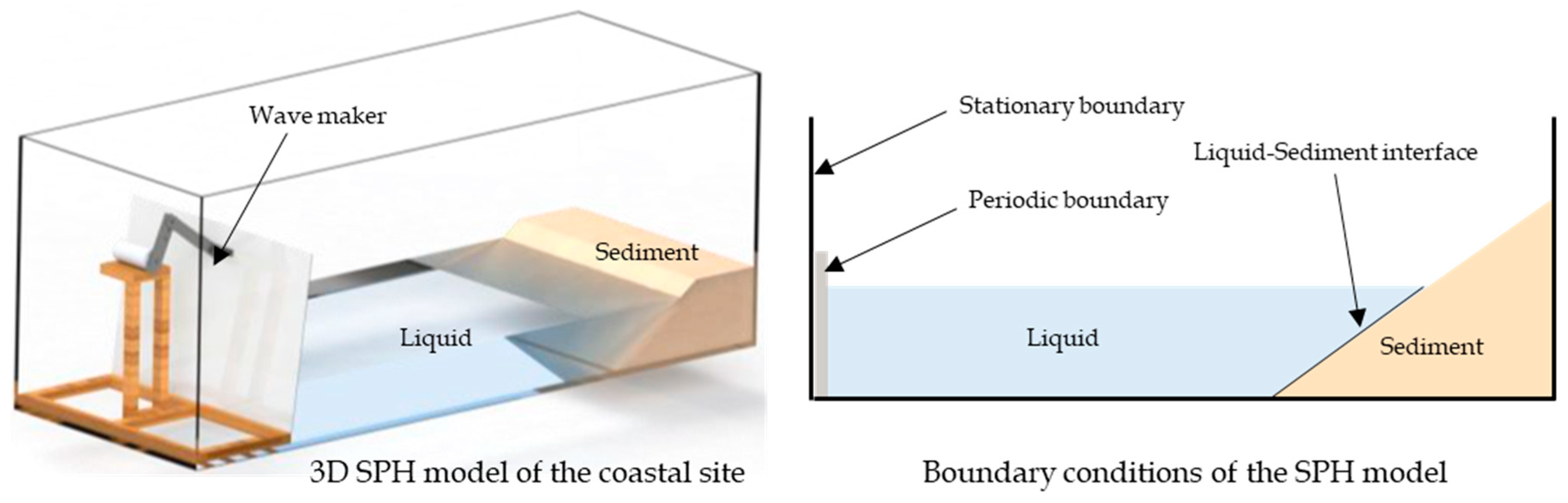
The 3D SPH model of the liquid–sediment interaction is created, as shown in Figure 4, based on the preliminary data obtained from the study site. The model uses seawater (liquid), sediment, and a wave maker to generate the sea wave. All structures at the site are included in the model to mimic the real coastal settings of the actual site. The topography of the site is also included in the model. The model is created using SolidWorks and then exported to SPH software and ANSYS to run the numerical analysis.

A stationary boundary condition is applied to the wall of the enclosed box; a periodic boundary is applied to the wave maker, which generates sea waves periodically; and an interface boundary is applied to the liquid–sediment interface. The particles are sorted in a staggered arrangement, with their position initially set as stationary.

Table 3. Material properties of the seawater and sediment.

Parameter	Liquid	Sediment
Density of Sea Water	${\rho }_0 =$ 1029 kg/m3	${\rho }_1 =$ 1922 kg/m3
Dynamic viscosity	${\mathsf{\mu }}_0 = 1.08\times {10}^{-3}$ Pa·s	${\mathsf{\mu }}_1 =$ 0.126 Pa·s
The numerical speed of sound in seawater	$C_{{s0}_0} =$ 80	$C_{{s0}_1} =$ 81
Polytropic index of seawater	${\gamma }_0 =$ 7	${\gamma }_1 =$ 7
Parameter $n$ of the Herschel–Bulkley–Papanastasiou model	$n_0 =$ 1	$n_1 =$ 1
Parameter $m$ of the Herschel–Bulkley–Papanastasiou model	$m_0 =$ 0	$m_1=$ 100
Cohesion coefficient	$c_0 =$ 0	$c_1 =$ 1
Internal friction angle	${\varphi }_0 =$ 0	${\varphi }_1 =$ 35

shows the material properties of the seawater and sediment, respectively.

Shear thinning occurs in the sediment phase; therefore, the HBP values are set to 1 and 100 (as shown in Table 3) to simulate such an occurrence. The value n will control the behavior of the shear-thinning non-Newtonian fluid, and the value of m will control the shear thickening. The cohesion coefficient, $c_1$ and internal friction angle, ${\varphi }_1$ are obtained through direct shear stress analysis. The selected marine sediment samples have densities between 0.95 and 2.60 kg/m³ [27]. The specific value is determined by factors such as marine conditions and voids in the sediment. This study’s sediment density and other parameters are based on the related literature [8,12,28].

The time-stepping algorithm is an explicit second-order predictor-corrector integrator method that predicts changes in time in half steps. The values are then amended using force at the half-time step [2,9]. The maximum force term and the numerical speed of sound will follow the form demonstrated by [26], which is restricted by the CFL condition:

$$\Delta t=C_0\mathit{min}\left(\sqrt{\frac{l_s}{\left|f_i\right|}}, \frac{l_s}{C_{s0}} ,\frac{l_s^2}{v}\right).$$

(14)

where min denotes the minimum function, $f_i$ is the force per unit mass of particle $i$, $C_0$ is the Courant number, and $v$ is the kinematic viscosity.

The parameter set-up of the SPH formulations is implemented through XML codes. In the XML coding, parameters such as the geometry of the liquid and the sediment systems, materials properties of the systems, boundary conditions, time stepping parameters, and other set-up properties are specified. The sediment particles are defined in the XML by specifying the lower and upper bounds of the particle sizes. Specifically, the study considers sand particles of smaller sizes (less than 0.2 mm) within the fine sand range. Based on the sieve analysis of the sediment samples obtained from the coastal site, sand particles of sizes 0.15 mm and 0.063 mm are used in the XML coding of the SPH. Other parameters of the setup are defined as explained in the formulations.

2.4. Model Scaling and Dimensionless Study

The physical hydraulic model is designed to have flow conditions similar to those at the actual coastal site. The model is designed to display geometric, kinematic, and dynamic similarities to the actual site. The relevant engineering drawings and survey plan of the river cross-sections are prepared to construct the scaled physical model. The geometric similarity is based on the site drawings, and the dynamic similarity is based on the Froude law. After examining the computed range of discharge, water depths, velocities, and other hydraulic parameters at the coastal site and the available space in the hydraulic laboratory, the model is constructed to a viable geometric scale to achieve appropriate measurements.

Factors such as reproducibility, flow supply to the test laboratory, test model space, and measurement convenience determine the scale of the hydraulic model. In general, river models have a smaller water depth in comparison to the length and width of the channel. Meanwhile, it is necessary to secure the maximum water depth considering the precision of the water level measurements in the model. Based on these conditions, a downscale model with horizontal and vertical scales of 1/25 of the beach site is adopted in this study. Meanwhile, the SPH numerical model is a 1–1 scale of the PIV experimental test.

2.4.1. Model Scaling

To obtain a geometric similarity between the hydraulic model and the coastal site, the Froude number of the model and the site must be the same for flow conditions where inertia and gravitational forces are dominant. For viscous forces, dimensional analysis is used to demonstrate that the Reynolds numbers of the model and the actual site are the same. The Froude and Reynolds numbers are defined as:

$$\mathrm{Froude} \mathrm{number}: F_n=\frac{V}{{(gL)}^{0.5}}$$

(15)

$$\mathrm{Reynolds} \mathrm{number}: R=\frac{VL}{K}$$

(16)

where $V$ is the velocity, $g$ is the gravitational acceleration, $L$ is the characteristic length, and $K$ is the kinematic viscosity. The scaling is performed using the Froude number, which is modified based on the wave propagation formulation as follows:

$$\mathrm{Velocity}: V=\lambda \times d_w\times f$$

(17)

$$\mathrm{Froude} \mathrm{number}: F_n=\frac{\lambda \times d_w\times f}{{(gL)}^{0.5}}$$

(18)

where $\lambda =H/L_0$ is the offshore wave steepness, with $H$ and $L_0$ denoting the offshore wave height and wavelength, respectively. $d_w$ is the water depth, and $f$ is the wave frequency. Therefore, the Froude numbers for the actual scale and the downscale are expressed as follows:

$$F_{n_{\mathrm{real}}}=\frac{{\lambda }_{\mathrm{real}}\times d_{w_{\mathrm{real}}}\times f_{\mathrm{real}}}{{(g{L}_{\mathrm{real}})}^{0.5}}$$

(19)

$$F_{n_{\mathrm{downscale}}}=\frac{{\lambda }_{\mathrm{downscale}}\times d_{w_{\mathrm{downscale}}}\times f_{\mathrm{downscale}}}{{(g{L}_{\mathrm{downscale}})}^{0.5}}$$

(20)

For model scaling, the Froude number of the actual scale must be equal to that of the downscale, as follows:

$$F_{n_{\mathrm{real}}}=F_{n_{\mathrm{downscale}}}$$

(21)

$$\frac{{\lambda }_{\mathrm{real}}\times d_{w_{\mathrm{real}}}\times f_{\mathrm{real}}}{{(g{L}_{\mathrm{real}})}^{0.5}}=\frac{{\lambda }_{\mathrm{downscale}}\times d_{w_{\mathrm{downscale}}}\times f_{\mathrm{downscale}}}{{(g{L}_{\mathrm{downscale}})}^{0.5}}$$

(22)

2.4.2. Dimensionless Study of Fluid Wave Breakers

In this work, two dimensionless numbers, namely the Iribarren and Froude numbers, are used to characterize and identify the type of sea (fluid) wave breaker encountered in the liquid–sediment interaction in the coastal site model. The Iribarren number is obtained as:

$$\xi =\sqrt{\frac{g{T}^2}{2\pi H}}·\tan \phi$$

(23)

where $T$ is the period, and $\phi$ is the angle of the seaward slope. The Froude number is applied to determine the resistance of a partially submerged object moving through the water. It is expressed as:

$$F_n=\frac{\lambda d_{w}f}{\sqrt{g\left(\frac{1}{\alpha }\right)}}$$

(24)

where $\alpha =\tan \phi$ is the seaward slope. The value 1 in Equation (24) denotes the magnitude of the wave height in the expression for the characteristic length $L=H/\alpha$.

3. Results and Discussion

3.1. Distance Particle Sensitivity Analysis

A sensitivity study of the distance particle (Dp) is conducted to determine the best Dp value for the SPH simulation model. The analysis uses a similar numerical model and set-up for different distance particles to assess the Dp, which yields optimal convergence accuracy and computational time. Distance particles with values of 0.002, 0.005, 0.01, 0.015, and 0.02 are considered in the analysis. The simulation is run for a period of 15 s. However, the lower the Dp value, the higher the number of particles in the SPH model, and hence the higher the computational time of the simulation. The optimum Dp value should have the best convergence accuracy at a considerable computational cost.

The average velocity magnitude computed using the different Dps for a simulation period of 15 s is shown in Figure 5. The line pattern for the average velocity of Dp-0.02 shows the highest disparity compared to the other Dps, which have nearly similar average velocity values. Additionally, among the similar Dps, the Dp-0.015-line pattern shows considerable differences at 4–5 s and 12–13 s. Based on these findings, Dp-0.01, Dp-0.005, and Dp-0.002 possess similar average velocity patterns and are potentially optimized Dp. As a further analysis, the $H_{SPH}/Dp$ ratio is computed for the three remaining Dps. According to [29], an optimized solution must be in the range of $H_{SPH}/dp\approx 8–10$ particles. With $H_{SPH}=0.1 \mathrm{m}$, Dp-001, with $H_{SPH}/dp=10$, is within the acceptable range compared to the other two Dps with ratio values of 20 and 50, respectively. Therefore, Dp-0.01 is the optimum Dp, which gives an optimum balance between computational time and convergence accuracy compared to the other Dp values. The Dp-0.01 model is hence adopted in the SPH simulation.

3.2. Flow Velocity Magnitude

Figure 6 compares the flow velocity magnitudes obtained through the particle image velocimetry experiment against those of the smooth particle hydrodynamics simulation. The experimental results are used as a benchmark to validate the accuracy and reliability of the simulation results. Both models are run for 20 s, and the fluid and sediment flow dynamics are observed at every 4 s time-step increment.

As observed in Figure 6, the fluid starts to erode the sediment profile from the top, starting at 4 s in both models. The maximum velocity magnitude of the flow is recorded as 0.5623 m/s and 0.5860 m/s for the simulation and the experimental models, respectively, with a percentage difference of only 4.21%. These observations infer good agreements between the experimental measurements and the numerical predictions and thus highlight the usefulness of the numerical methodology.

Moreover, a detailed profile of the liquid–sediment interaction is shown in Figure 7, which presents the elevation of the liquid and beach (sediment) profiles between the length range of 0.93 m and 1.07 m. As modeling time progresses, more water waves are generated, which results in more significant erosion of the beach (sediment) profile and hence a reduction in the elevation of the sediment profile.

Qualitatively, the fluid and sediment profiles of the PIV experiment are in good agreement with those of the SPH simulation, as shown in Figure 7. The level of similarity obtained demonstrates that the reliability of the developed SPH numerical model and the PIV experiment is within an acceptable range. Meanwhile, achieving an exact qualitative agreement between the numerically and experimentally computed liquid–sediment profiles is difficult due to some limitations contributing to the disparity recorded in the results. These factors include the generated noise during the PIV experiment and the assumption of controllable flow and perfect environmental conditions in the SPH simulation, compared to the uncontrollable flow and ambient environmental conditions of the PIV experiment.

In addition, the flow velocity magnitude is investigated at five different locations within the fluid domain, as shown in Figure 8. The results of the investigation are presented in Figure 9 and

Table 4. $ℒ1$ and $ℒ2$ norms of the velocity hydrographs obtained at the probe locations.

Probe	Coordinate		$\mathbf{ℒ}1 \mathbf{Norm}$			$\mathbf{ℒ}2 \mathbf{Norm}$
Point	y (mm)	z (mm)	PIV Exp.	SPH Sim.	Diff (%)	PIV Exp.	SPH Sim.	Diff (%)
1	984.22	95.99	2.09	1.98	5.37	1.60	1.53	4.42
2	954.94	76.14	3.07	3.04	0.96	2.29	2.23	2.33
3	935.09	49.95	2.25	2.24	0.27	1.66	1.66	0.15
4	908.09	67.19	2.26	2.30	1.95	1.66	1.71	2.88
5	920.95	93.87	2.61	2.51	3.92	1.93	1.87	3.07

. Table 4 also presents the coordinates of the probe locations. The locations are probed using the PIV and SPH approaches to establish more validation for the simulation approach. The velocity hydrographs obtained at the probe points using the two methods are shown in Figure 9, while Table 4 presents the computed $ℒ1$ and $ℒ2$ norms of the velocity hydrographs. The norms are calculated to investigate the difference in the velocity magnitudes obtained through the PIV experiment and the SPH simulation.

As shown in Figure 9, higher flow velocity magnitudes are observed at locations 1, 2, and 5 compared to locations 3 and 4. This observation establishes that flow velocity near the upstream is higher than the downstream. Maximum and minimum percentage differences of 5.37% and 0.27% are observed in the $ℒ1$ norm values of the velocity hydrographs. On the other hand, maximum and minimum percentage differences of 4.42% and 0.15% are recorded in the $ℒ2$ norm values of the hydrographs. Moreover, the hydrographs of probe point 2 exhibit the highest norm values, while the lowest norm values are obtained at probe point 1. These trends, as well as those of the other probe points, are maintained in the results of both methods and the two norm values. Based on these findings, it can be admitted that the usefulness of the SPH numerical methodology has been further established for the current liquid–sediment interaction study case.

3.3. Breaking Wave Characteristics of the Liquid–Sediment Interaction

The breaking wave characteristics of the liquid–sediment interaction are studied using two dimensionless numbers, namely Iribarren and Froude numbers. Based on the dimensionless analysis presented in Section 2.4, the dimensionless numbers are proportional to the sea wave frequency $f$ and the angle of the seaward slope $\alpha$. The influence of the frequency and the slope on the dimensionless numbers, and hence the breaking wave characteristics, is studied.

The SPH model of the liquid–sediment interaction is studied for ten different wave frequencies ranging between 0.1 Hz and 1.0 Hz, and the effect of the frequency value on the Iribarren number is investigated. The wave height is taken from the surf break region due to its better accuracy than the offshore region [30]. The results obtained are presented in Figure 10. It is observed that the Iribarren number decreases as the wave frequency increases, which is well-fitted into a decaying power-law curve at a high coefficient of determination, $R^2$. The Irribarren numbers computed fall within the range $\xi >2.0$ for wave frequencies $f<0.15$ Hz, $0.4<\xi <2.0$ for wave frequencies $0.15<f<0.55$ Hz, and $\xi <0.4$ for wave frequencies $0.55<f\le 1.0$ Hz. According to [30], the observed results denote that the breaking wave characteristic is surging or collapsing at the wave frequency range of $f<0.15$ Hz, plunging at the wave frequency range of $0.15<f<0.55$ Hz, and spilling at the wave frequency range of $0.55<f\le 1.0$ Hz.

The breaking wave characteristics of the liquid–sediment model is further investigated by considering the influence of the seaward slope angle on the breaking phenomenon. Froude numbers are calculated using the wave frequencies presented in Figure 11, according to Equation (16). The computation is made for different values of slope angle $\phi$, which ranges from $10°$ to $70°$, to investigate its influence on the breaking wave characteristics. The computed Froude numbers are then plotted against the Iribarren number using the relationship between the wave frequency and the Iribarren number. Figure 11 presents the plot of the Iribarren number against Froude for different magnitudes of the seaward slope angle.

Generally, the Iribarren number decreases with an increment in the magnitude of the Froude number. This increment is consistent with the earlier observation; since the Iribarren number is inversely proportional to the wave frequency, and the Froude number is directly proportional to the wave frequency (according to Equation (24)), it is expected that the Iribarren number be inversely proportional to the Froude number. Furthermore, the Iribarren and Froude numbers are directly proportional to the seaward slope angle, as shown in Figure 11. The higher the slope angle, the greater the tendency to produce a surging/collapsing breaking wave phenomenon. The lower the slope angle, the greater the tendency to produce a spilling wave breaker. This observation infers that a higher slope results in a higher contact force between the fluid and the sediment and thus increases erosion tendency. Moreover, at a particular Froude number, it is observed that spilling, plunging, and surging wave breakers are produced at low, mid, and high seaward slope angles, respectively. Meanwhile, increasing the Froude number increases the tendency to produce spilling or plugging wave breakers, irrespective of the slope angle.

Based on the results presented in Figure 10 and Figure 11, it can be inferred that the wave frequency and the seaward slope angle greatly influence the breaking wave characteristics of a coastal liquid–sediment interaction.

4. Conclusions

This paper investigated a coastal area’s fluid flow and liquid–sediment interaction using the particle image velocimetry (PIV) experiment and the smooth particle hydrodynamics (SPH) numerical method. A simplified physical model of the study site near the Tuanku Jaafar power station was developed using the data and materials obtained from the site. The PIV experimental suite was set up on the physical model to analyze the fluid and sediment profiles and the velocity magnitude of the fluid flow. The obtained results were compared against those obtained through the SPH simulation. Further analysis was conducted to study the breaking wave characteristics of the coastal liquid–sediment interaction and establish the wave frequency and seaward slope angle impacts. The study’s main findings are as follows: (a) The maximum velocity magnitude of the flow is recorded as 0.5623 m/s and 0.5860 m/s for the simulation and the experimental models, respectively, with a percentage difference of only 4.21%. (b) The fluid and sediment profiles obtained through the PIV experiment and the SPH simulation are close, which further justifies the usefulness of the simulation approach. (c) The flow velocity near the upstream region is higher than the coastal model’s downstream region. With maximum percentage differences of 5w.37% and 4.42% in the $ℒ1$ norm and $ℒ2$ norm values, between the experimental measurements and the numerical predictions of the flow velocity hydrographs at different locations; it can be admitted that the usefulness of the SPH numerical methodology is further established for the liquid–sediment interactions study. (d) It was found that the Iribarren number of the fluid interaction with the sediment is inversely proportional to the sea wave frequency. The wave breaker characteristic is surging or collapsing at the wave frequency range of $f<0.15$ Hz, plunging at the wave frequency range of $0.15<f<0.55$ Hz, and spilling at the wave frequency range of $0.55<f\le 1.0$ Hz. (e) Additionally, the Iribarren number is inversely proportional to the Froude number, and both are directly proportional to the seaward slope angle. At a particular Froude number, it is observed that spilling, plunging, and surging wave breakers are produced at low, mid, and high seaward slope angles, respectively. Meanwhile, increasing the Froude number increases the tendency to produce spilling or plugging wave breakers, irrespective of the slope angle.

The developed downscale PIV laboratory tests and the SPH simulations predict the liquid–sediment system interactions at an acceptable limit. However, when they are employed in modeling full-scale coastal systems, underestimations of the flow dynamics parameters can be expected. Meanwhile, dimensional analysis is applied to achieve dynamic and geometric similitudes between the developed downscale model and the full scale. Additionally, limitations such as the generated noise during the PIV experiment and the assumptions of controllable flow and perfect environmental conditions in the SPH simulation contribute to the slight disparity between the PIV measurements and the SPH predictions. Implementing uncontrollable flow conditions in the SPH simulation and eliminating noise generation in the PIV experiment are vital to ameliorating this drawback. The work presented in this paper can be extended to a larger scale model to further study the relationship between sediment transport, Iribarren and Froude numbers, and the effect of marine waves on sediment transport.

Lastly, the paper has demonstrated the developed SPH methodology’s usefulness in predicting a coastal liquid–sediment system’s flow and interaction properties.