Article

Experimental and Modeling Evaluation of Impacts of Different Tillage Practices on Fitting Parameters of Kostiakov’s Cumulative Infiltration Empirical Equation

by
Mahmoud Abdel-Sattar
1,*,
Rashid S. Al-Obeed
1,
Saad A. Al-Hamed
2 and
Abdulwahed M. Aboukarima
2
1
Department of Plant Production, College of Food and Agriculture Sciences, King Saud University, P.O. Box 2460, Riyadh 11451, Saudi Arabia
2
Department of Agricultural Engineering, College of Food and Agriculture Sciences, King Saud University, P.O. Box 2460, Riyadh 11451, Saudi Arabia
*
Author to whom correspondence should be addressed.
Water 2023, 15(14), 2673; https://doi.org/10.3390/w15142673
Submission received: 5 June 2023 / Revised: 6 July 2023 / Accepted: 15 July 2023 / Published: 24 July 2023

Abstract

:
The evaluation and modeling of the water infiltration rate into the soil are important to all aspects of water resources management and the design of irrigation systems for agricultural purposes. However, research focused on experimental studies of infiltration rates in clay soils under different tillage practices remains minimal. Therefore, an empirical prediction model for cumulative water infiltration needs to be created to estimate water depth under different tillage practices. Thus, the present research investigated the impacts of different tillage practices, including plow type (three tillage systems: moldboard, disk, and rotary plows), tillage depth (100 and 200 mm) and four soil compactions levels (0, 1, 3, and 5 tractor wheel passes), on cumulative infiltration behavior in a clay soil under a randomized complete design with three replications. Double-ring infiltration experiments were conducted to collect infiltration data. The research was conducted in three different stages. The first stage was performed through a field test to obtain infiltration data, the second stage involved using a Kostiakov empirical equation (Z = q × tb) for cumulative infiltration to acquire the fitting parameters of “q” and “b”, and in the last stage, we predicted the fitting parameters of “q” and “b” based on soil mean weight diameter, tillage depth, and four soil compaction levels by applying regression data mining approaches in Weka 3.8 software. The results show that the effects of relevant factors on the cumulative water infiltration depth of the soil could be statistically significant (p < 0.05). The Kostiakov model, with an average coefficient of determination of 0.939, had a good fitting effect on the cumulative water infiltration depth process of the investigated soil. The average, lowest, and maximum values of the “q” parameter were 2.7073, 2.2724, and 3.1277 mm/minb, respectively, while for the “b” parameter, they were 0.5523, 0.5424, and 0.5647, respectively. Furthermore, the evaluation of several regression data mining approaches determined that the KStar (K*) data mining approach, with a root mean square error of 0.0228 mm/minb, a mean absolute error of 0.0179 mm/minb, and a correlation coefficient of 0.997, was the most accurate method for fitting parameter “q” using the testing dataset. The most accurate method for fitting the parameter “b” estimation was determined to be the Multilayer Perceptron method, with a root mean square error of 0.0026, a mean absolute error of 0.0013, and a correlation coefficient of 0.962, using the testing dataset. Therefore, this research, which consisted of in situ field observation experiments and infiltration modeling of the infiltration process in a clay soil, provides an essential theoretical basis for improving models of the rate of cumulative infiltration. Moreover, the proposed methodology could be employed for simulation of the fitting parameters “q” and “b” for soil water cumulative infiltration processes, not only for irrigation management purposes under regular crop production conditions, but also for the selection of the most suitable tillage practices to modify the soil during the agriculture season to conserve water and prevent yield declines. The results support the understanding of the infiltration processes in a clay soil and demonstrate that tillage practices could reduce the water infiltration rate into the soil.

1. Introduction

The infiltration process, which is crucial for designing irrigation and drainage systems, evaluating groundwater recharge and contamination, managing floods and droughts, etc., is frequently influenced by a number of variables, with soil use, soil cover, and soil physical characteristics being the main ones [1]. Hydrologists and water managers face a major challenge because of the considerable spatial variability that these factors cause in the infiltration process. Therefore, the soil infiltration water characteristics under various tillage practices for soil preparation for crop output must be defined. These characteristics are crucial for the construction of irrigation systems [2]. Due to the impact of soil use variation on the spatial changeability of infiltration parameters, numerous trials and theoretical investigations have been performed that aim to understand the links between infiltration processes and various agricultural management practices, in particular tillage operations [3] as they alter soil structure by creating macrospores that significantly affect the water infiltration rate into soil [4,5,6,7].
The most serious environmental challenge resulting from modern agriculture is thought to be soil compaction. Wheeled farm equipment handles the majority of the typical tasks involved in conventional agriculture. The weight of the tractor and the attached machinery compacts the soil during these activities [5]. Numerous research papers have examined the impacts of soil management procedures like soil compaction and tillage on the characteristics of water infiltration into soil [3,8]. Soil compaction reduces pore space, creating a dense soil with poor internal drainage and decreased aeration, which increases soil strength and impedes root development in particular [5]. Furthermore, increasing tillage depth from 150 to 450 mm showed increases in cumulative infiltration, indicating that tillage depth has an observable impact on the water cumulative infiltration in a soil [7]. The rate of water infiltration into the soil also rises as tillage depth increases [9]. Furthermore, the effects of diverse soil use and agricultural management procedures on the water infiltration into the soil have been examined, showing the substantial influence of soil use modification [10].
The effectiveness of irrigation methods and water use efficiency is directly impacted by estimations of the infiltration characteristics of the soil. The most suitable approach for calculating experimental infiltration models parameters can change in the same soil owing to the difficulty in determining parameters without in situ experiments [11,12]. To determine water infiltration into the soil, a number of empirical models have been developed. The water infiltration into the soil can be given as a function of infiltration time and other empirical constants. Kostiakov, modified Kostiakov, and Horton [13] are the empirical models most commonly used in infiltration data analysis. However, due to its variability within the field, predicting water infiltration into the soil is a major challenge. A suitable empirical model is required to establish the model’s parameters created on the properties of a limited soil [14]. Thus, an innovative model needs to be developed to make better decisions and allow irrigation engineers to study the different impacts of tillage practices on accumulated water depth in the field. Additionally, determining the amount of infiltration is essential for estimating the extra water required for irrigation and determining whether water is available for crop development [15]. Additionally, the water infiltration rate into soil is a crucial measure of irrigation and drainage effectiveness, improved plant water accessibility, increased yields, decreased erosion, and water wastage [16]. As a result, irrigation researchers have given the study of the infiltration process much focus [17,18]. Equally, numerous approaches have been developed to identify model parameters for various soil situations [14]. For instance, the water cumulative infiltration (Z, mm) and infiltration time values (t) were subjected to a nonlinear regression examination ( Z = q × t b ) to identify parameters “q” and “b” in the Kostiakov model [14]. According to convention, the parameter of “b” is higher than zero but less than one [19], “b” indicates the constancy of the soil’s structure, and “q” is a measure of the soil’s initial rate of water infiltration and soil structural conditions [20]. Additionally, Elmarazky et al. [21] established a model with R2 values of 0.902 and 0.765 to obtain the “k” and “u” parameters, respectively, of the Kostiakov equation ( I = k × t u ) for infiltration rate (I) in units of mm/h, employing the multiple linear regression (MLR) method. In their model, the soil mean weight diameter, the number of tractor wheel passes on the surface of the plowed soil, and the tillage depth were used as inputs. Hossne García et al. [22] conducted field experiments to study the effects of wetness, soil depth, and compaction on infiltration rate (mm/h) and employed the Kostiakov equation ( I = k × t u ) for infiltration rate (I) in units of mm/h to acquire the Kostiakov fitting parameters “k” and “u”. They then employed the MLR method to model these two fitting parameters. Al-Sulaiman et al. [23] employed MLR to formulate the Kostiakov parameters “q” and “b” for water cumulative infiltration of the Kostiakov model. In their MLR model, the water electric conductivity, soil texture index, initial soil bulk density, soil sodium adsorption ratio, initial soil moisture content, soil electric conductivity, water sodium adsorption ratio, and organic matter percentage in the soil were used as inputs.
Although some prior research on cumulative infiltration modeling using data mining algorithms has been conducted [24,25], no research has focused on developing models for infiltration model parameters, despite the fact that these parameters are crucial for appraising the performance behavior of soil water infiltration models [26]. Artificial neural networks have been used (ANN) to predict water infiltration [13,24,25,27,28]. Some researchers applied machine-learning tools to predict infiltration rates [24,25,28,29,30,31,32,33]. Others employed the adaptive neuro-fuzzy inference system (ANFIS) to model soil water infiltration [24,28,34]. In order to estimate the amount of infiltrated water in the furrow irrigation method, Sayari et al. [35] proposed five common artificial intelligence models, including ANN, ANFIS, MLR, Group Method of Data Handling, and Support Vector Regression. Data for evaluating these artificial intelligence models were collected from field tests and the available literature. The advance time at the end of the furrow, inflow rate, furrow length, cross-sectional area of inflow, and infiltration opportunity time were used as the input factors in the simulation.
Evaluation and modeling of water infiltration rate into the soil are important to all aspects of water resources management and the design of irrigation systems for agricultural purposes. On the other hand, research focused on experimental studies of infiltration rates in clay soils under different tillage practices remains minimal. Therefore, this research was conducted in three stages. The goal of the first stage was to conduct an experimental study investigating the impacts of the number of tractor wheel passes on clay soil in three tillage systems (moldboard, chisel, and rotary plows) under two tillage depths on the cumulative infiltration depth. Additionally, in the second stage of the research, the infiltration parameters of the clay soil were determined and assessed using Kostiakov’s cumulative infiltration model ( Z = q × t b ). In addition, the aim of the third stage of the research was to test the efficacy of several data mining approaches for predicting the parameters of “q” and “b”, utilizing experimental field data for a clay soil. Accurate “q” and “b” predictions are crucial and would undoubtedly assist irrigation engineers to design irrigation and drainage systems, etc. The eight regression algorithms (M5Rules, Additive Regression, KStar (K*), SMOreg, Multilayer Perceptron (MLP), Linear Regression (LR), and Gaussian Processes) within the Waikato Environment for Knowledge Analysis (Weka) 3.8 software were employed to predict the parameters “q” and “b”.

2. Materials and Methods

The present research investigated the impacts of different tillage practices, including plow type (three tillage systems, moldboard, disk, and rotary plows), tillage depth (100 and 200 mm), and four soil compactions levels (0, 1, 3, and 5 of tractor wheel passes) on cumulative infiltration behavior in a clay soil under a randomized complete design with three replications. Double-ring infiltration experiments were conducted to collect infiltration data. The research consisted of three different stages. The first stage was a field test to obtain infiltration data, the second involved the application of the Kostiakov empirical equation ( Z = q × t b ) for cumulative infiltration to acquire the fitting parameters of “q” and “b”, where Z is cumulative infiltration (mm), and t is infiltration time. The last stage involved prediction of the fitting parameters of “q” and “b” based on soil mean weight diameter, tillage depth, and four soil compactions levels by applying regression data mining approaches in Weka 3.8 software. The procedures employed have been reported previously in [21,22]. However, the details of the procedures in this research are discussed below.

2.1. Procedures of the First Stage of the Research (the Experimental Work)

The infiltration experiments were located at the Rice Mechanization Center’s Research Farm in Meet El Deeba, Kafr El-Sheikh, Egypt (longitude: 30°51′17.6″ E and latitude: 31°06′59.3″ N), and the soil water infiltration trials were carried out in a clay field. Four soil samples were collected from a nearby location and used to analyze the characteristics of the soil. The average percentage sand, silt, and clay contents at the experimental site for two soil depths can be seen in Figure 1. The soil bulk density was observed at two soil depths (0–150 mm and 150–300 mm), with values of 1.12 and 1.21 g/cm3, respectively. The experiments were conducted on an area of 0.405 ha. Water was applied to the test area, and it was then permitted to dry out until the soil moisture content was between 15% and 19% db.
In this research, various tillage practices were investigated. Three distinct tillage methods—moldboard, chisel, and rotary plows—were used for soil tillage. These were applied in order to obtain various levels of soil aggregation as indicated by the mean weight diameter (MWD) of the soil. Furthermore, two tillage depths were applied during soil tillage. The tractor wheels passed on the plowed soil surface to apply four levels of compaction (soil compaction level-0, soil compaction level-1, soil compaction level-3, and soil compaction level-5). The specifications of the tillage implement used in the experiments are provided by Elmarazky et al. [21]. However, the three treatments were established statistically in a randomized complete design with three replications. The levels of soil compaction were applied by driving an agricultural tractor with mass of 4840 kg (without any implement behind it) over the plowed soil surface with a forward speed of 4.5 km/h. Two tillage depths were applied in the range of 100–200 mm. The plots in the experimental site had an area of 30 m × 2.5 m. To avoid overlapping among treated plots, a 1 m spacing between the treated plots was retained as a buffer. Five kg soil samples were collected along three arbitrarily chosen transects of each plot at different tillage depths, after both the tillage and traffic treatments. After air-drying of the samples, they were sieved with standard sieves to determine the defined size distribution of soil aggregates [36]. The product of the aggregate diameters in each sieve size and the proportionate weight of soil aggregate in that sieve size were added to define the soil mean weight diameter (MWD) [37] as follows:
M W D = i = 1 n X i × W i
where Xi is the average diameter of the aggregate class (mm), n is number of sieves, and Wi is the proportion of each aggregate class in relation to the total aggregate weight.

2.2. Double-Ring Infiltration Experiments

Infiltration rates were observed using a cylindrical infiltrometer. The cylindrical infiltrometer (double-ring infiltrometer) had two rings with a length of 450 mm and the inner diameter was 300 mm for each ring. The two rings were inserted into the soil to a depth of around 70 mm using a rubber hammer with a weight which hit a wooden board attached to ring wall consistently without disturbing the soil surface. The two rings were filled with water to an equivalent depth, and the opening reading of the water level was observed. The experimental water used to measure the soil water infiltration rate was similar to that used for irrigating purposes in the site. A fixed 200 mm head of water was kept in each loop and the infiltration measurements were noted and documented for five minutes. Readings were made at regular time intervals for 3 h (180 min). The soil water infiltration rate was then calculated from the collected infiltration data and infiltration time to obtain the rate of infiltration in units of mm/h, and then the water cumulative infiltration depth (Z, mm) was calculated.

2.3. Determination of Kostiakov Equation Fitting Parameters for Cumulative Infiltration (the Second Stage of the Research)

In most water infiltration experiments, the most generally employed empirical model is the Kostiakov model, which has a few simple calculations [17]. Kostiakov [38] presented his model early for determining the water cumulative infiltration depth as follows:
Z = q × t b
where Z is the water cumulative infiltration depth (mm) at time interval t (minutes) and “q” is fitting constant called the soil infiltration coefficient (mm/minb), and “b” is the experimental fitting constant called the infiltration index constant (dimensionless). However, “q” and “b” are fitting parameters that are site-specific and depend on soil conditions such as soil bulk density, soil texture, soil moisture content, and other soil properties [39]. As the Kostiakov infiltration equation is empirical, no physical implications are involved in its related fitting parameters [40].
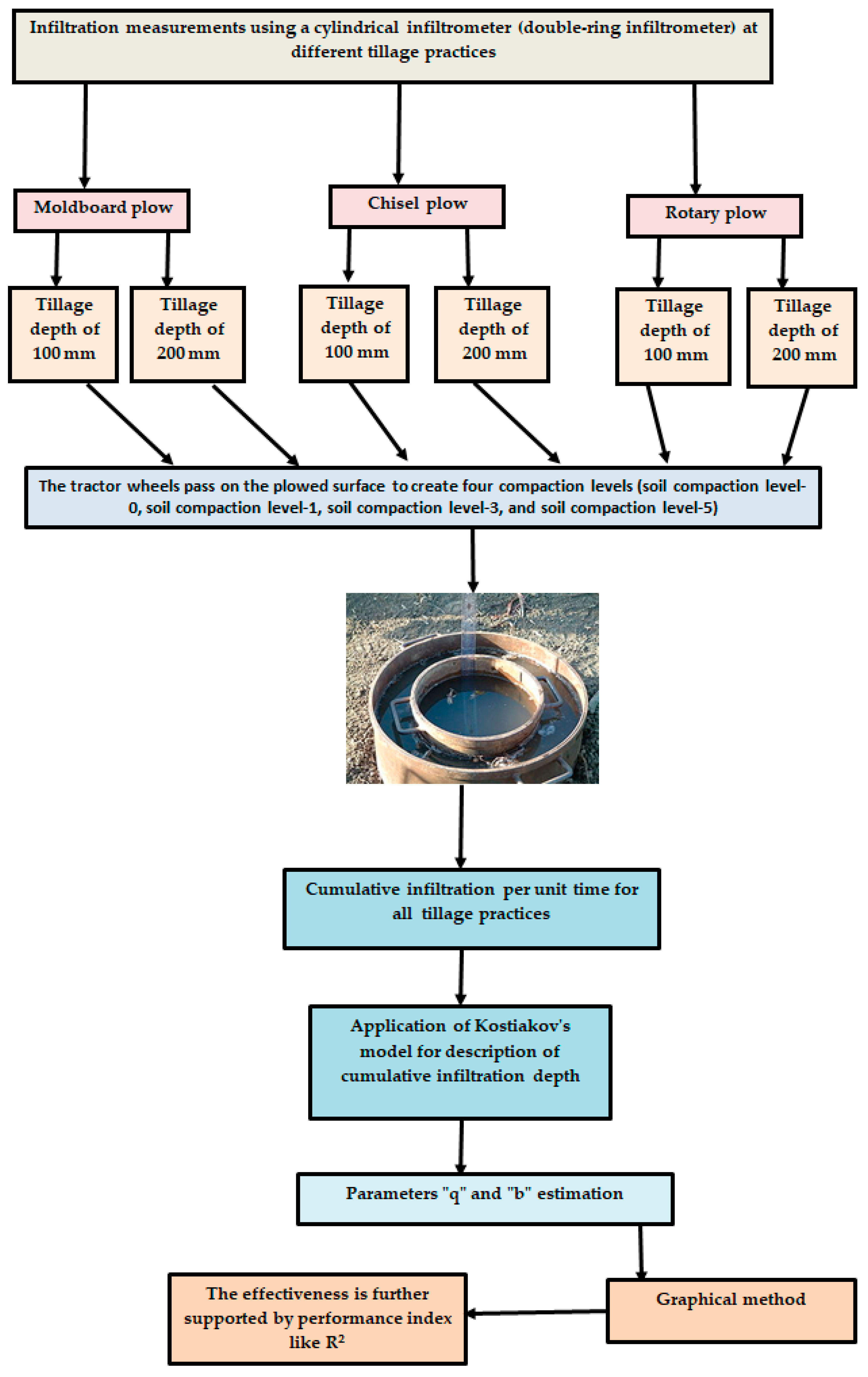
Using logarithmic transformation [41] and field experimental data, the Kostiakov equation’s linearized pattern was employed. Using this traditional method, which is called a graphical method, the fitting parameters of “q” and “b” in the Kostiakov model (Equation (2)) were determined by fitting a regression line to a plot curve of ln (Z) against ln (t). The intercept of the best-fit regression line on the ordinate axis then signifies the value of ln (q) and its slope is equivalent to “b” [26], where “q” and “b” are the Kostiakov model parameters such that “q” is greater than 0, while ”b” is greater than 0 and less than 1 [19]. In the present research, 42 observations for “q” and “b” were determined from the field experiment infiltration data with a high coefficient of determination (R2 was greater than 0.938). Figure 2 shows the steps in the research methodology for obtaining the fitting parameters “q” and “b”.

2.4. Statistical Analysis

The effects of various tillage implements, levels of soil compaction, and tillage depth on MWD and fitting parameters “q” and “b” were assessed by analysis of variance (ANOVA) table in three ways, for a randomized complete design with three replicates using SAS [43]. Mean values were compared using the least significant differences (LSD) at a significance level of 0.05.

2.5. Procedures of the Third Stage of the Research (Data Mining Algorithms)

This research employs the open source tool Weka 3.8, software written in Java (3.6.14 version) [44], to develop different computational models, which apply diverse regression techniques. Weka 3.8 software [45] is a fit-maintained computational method that includes a set of well-organized regression or classification algorithms that produce good outcomes in several fields. In this research, the regression tools inside Weka 3.8 software were utilized to predict the Kostiakov model parameters for cumulative infiltration, “q” and “b” (Equation (2)). The inputs included: MWD, ranging from 9.2 to 80.2 mm; the amount of tractor wheel traffic on the plowed soil surface (dimensionless) with 0, 1, 3, and 5 passes; and the tillage depth, ranging from 97 to 204 mm. The outputs were “q” and “b”. Weka provides ready-to-use tools in a range of machine learning procedures suitable for solving numerous data mining tasks. To achieve our goal, we relied on the field results for “q” and “b”. Weka has a simple and free-to-use graphical window to compare the outcomes of the different regression algorithms [46]. In the learning stage, a regression equation is created from the learning cases nominated by Weka. Table 1 provides short explanations of each of the regression algorithms used, for different classes, as initially defined by Weka [47]. Figure 3 depicts a flowchart for modeling “q” and “b” using the Weka software. WEKA was directed to select 66% of the data as the training dataset (28 points) and the remaining data were used for testing purposes (14 points).
The MLR method is employed to examine the linear relationship between one dependent factor and two or more independent factors [51]. However, this method in Weka is called linear regression (LR). In this research, the Kostiakov model parameters for water cumulative infiltration, “q” and “b”, as shown in Equation (2), were modeled using MLR based on MWD, tillage depth, and the number of tractor wheel passes on the plowed soil surface as inputs. MLR was completed using Weka software to obtain the regression constants ( 0 , 1 , 2 ,   a n d 3 ) in Equation (3) with the following relation:
q   o r   b = 0 + 1 ×   M W D + 2 ×   N T T + 3 ×   T D
where MWD is the soil weight mean diameter, NTT is the number of tractor wheel passes on the plowed soil surface (dimensionless) with 0, 1, 3, and 5 passes, and TD is the tillage depth.
Weka implements ridge regression and utilizes the standard least-squares linear regression method to obtain regression constants [52]. However, ridge regression is employed to solve difficulties that are not well displayed, which is significant when they have a poor chance of being resolved by a stable algorithm [53]. During the application of Weka regression algorithms, no attribute selection measure is required to accomplish the linear regression. Furthermore, in Weka, an artificial neural network called Multilayer Perceptron (MLP) is utilized. MLP is one of the most well-known data-driven technologies and is stimulated by the operations of the nervous system and brain [54]. It is based on a feed-forward ANN. It consists of one input layer, one or more hidden layers, and one output layer. However, each layer is composed of several neurons and the likely connection between these layers denotes the link between the nodes. The input layer, which contains neurons equivalent to the total number of the input parameters, allocates the data displayed on the network and does not assist in the processing operation. This layer tracks one or more hidden layers that support data processing. The output layer is the final layer, which provides the final output. When the input layer is exposed to the value of inputs passing through the link between the neurons, these values are multiplied by the equivalent weight and aggregated to obtain the net output (Zj) of the unit as follows:
Z j = W i j × y i
where Wij is the weight of the link from unit i to j, yi is the input value at the input layer, and Zj is the output obtained by the transfer function to yield an output for unit j. Haykin [54] has provided a detailed discussion about ANN. In the current research, a three-layer feed-forward ANN based on the back propagation algorithm was employed, which is the default in Weka 3.8 software.

2.6. Statistical Criteria for Evaluation of Regression Data Mining Algorithms

A model trained on a training set can be assessed using multiple statistical approaches comparing the predictions with the real values in the testing dataset. The root mean squared error (RMSE) and mean absolute error (MAE) are some of these statistical criteria. Since it measures how closely the data match the fits regression line, the correlation coefficient or coefficient of determination (R2) is also used to compare the predictions with the real values in the testing dataset. In addition, R2 is a statistical procedure that identifies the proportion of a component’s variability that can be caused or explained by its relationship to another factor. The chosen metrics are the most well-known and widely applied success metrics [55]. The statistical criteria are computed as follows:
R M S E = i = 1 N P i O i 2 N
M A E = i = 1 N P i O i N
In Equation (5), Pi and Oi are the predicted and calculated “q” or “b” values, respectively, and N is the total number of readings.

3. Results and Discussion

3.1. Data Analysis of the First Stage of the Research (the Experimental Work) for Soil Mean Weight Diameter

Water infiltrates rapidly into granular soils but very slowly into massive and compact soils, suggesting that tillage practices can alter the soil structure and thereby alter the infiltration rate [56]. Moreover, soil with large particle sizes has a high infiltration rate [57,58]. Figure 4 shows how the typical MWD varied for rotary, moldboard, and chisel plows under different treatments. It was observed that MWD in the moldboard plow plots was in the range of 34.5 mm to 80.2 mm, and in the chisel plow plots, it was in the range of 19.6 mm to 45.7 mm, while it was in the range of 9.2 mm to 21.5 mm for the rotary plow plots. A summary of the ANOVA analysis demonstrating the effects of tillage implements, number of wheel passes and tillage depth and their interactions on mean weight diameter is shown in Table 2. The tillage implements, soil compaction level (number of wheel traffic passes) and tillage depth had significant effects (p < 0.05) on MWD. The average MWD for the moldboard plow treatment had the greatest value at 57.86 mm, while the average MWD for the chisel and rotary plot treatments had lower values of 32.98 mm and 15.50 mm, respectively (Table 3). Compared with other plowing implements, the moldboard plow created larger clods; thus, it had a greater MWD value than the other tillage implements. However, moldboard plowing can destroy the pore permanency and aggregate constancy, causing remains mobilization, erosion, and surface strengthening [59]. Similarly, Khadr [60] showed that a significant effect on MWD was seen when using tillage implements. Their MWD values in a clay soil were 71.98, 44.49 and 23.97 mm for moldboard, chisel, and disk harrow plows, respectively. In addition, the MWD values were higher under a tillage system consisting of a moldboard plow plus disk plow than under a chisel plow plus disk plow system [61]. However, Çarman [62] claimed that a moldboard plow created a higher MWD than a rotary tiller plow, heavy globe disk plow, and stubble cultivator plow. Furthermore, a moldboard plow yielded the highest MWD (34.78 and 10.05 mm), whereas a chisel plow yielded the lowest MWD (17.16 and 6.08 mm) when the plowing process was conducting on a loam soil at different plowing speed and the tillage depth was 200 mm [63]. Carter [64] observed that chisel plow aggregates were larger than moldboard plow aggregates.
Tillage depth significantly affected the soil aggregate mean weight diameter values. As seen in Table 3, tillage depth increased, and MWD decreased. Naseer et al. [65] reported that an increase in tillage depth from 100 mm to 200 mm, increased MWD by 9.01% after plowing by primary tillage implements. Similarly, increasing tillage depth from 100 to 150 and to 200 mm produced significant increases in MWD of 7.37% and 7.86%, respectively, after plowing with a chisel plow in a silty clay loam soil. In addition, increasing the tillage depth led to increased values of MWD [66]. Additionally, the maximum MWD was observed at tillage depths of 200–300 mm and the minimum at tillage depths of 100–200 mm [67].
As the compaction level increased, the MWD values decreased. With no compaction (soil compaction level-0), the MWD was 47.84 mm; for one pass of wheel traffic (soil compaction level-1), the MWD was 40.67 mm; for three passes (soil compaction level-3), the MWD was 30.52 mm; and for five passes (soil compaction level-5), the MWD was 22.76 mm (Table 3). These findings are in agreement with those of Ramezani et al. [67], who observed that the control treatment had the highest MWD and eight-wheel tractor traffic had the lowest MWD for loam, sandy and sandy loam soils. Higher traffic levels of agricultural machinery may lead to the creation of smaller aggregates, particularly under dry soil conditions [68]. Furthermore, after a single-pass tillage operation with a rotavator plow in a sandy loam soil, it was found to be 4.9 mm, and it was 14.54 mm for a moldboard plow [69].

3.2. Data Analysis of the Second Stage of the Research (Water Cumulative Infiltration Depths)

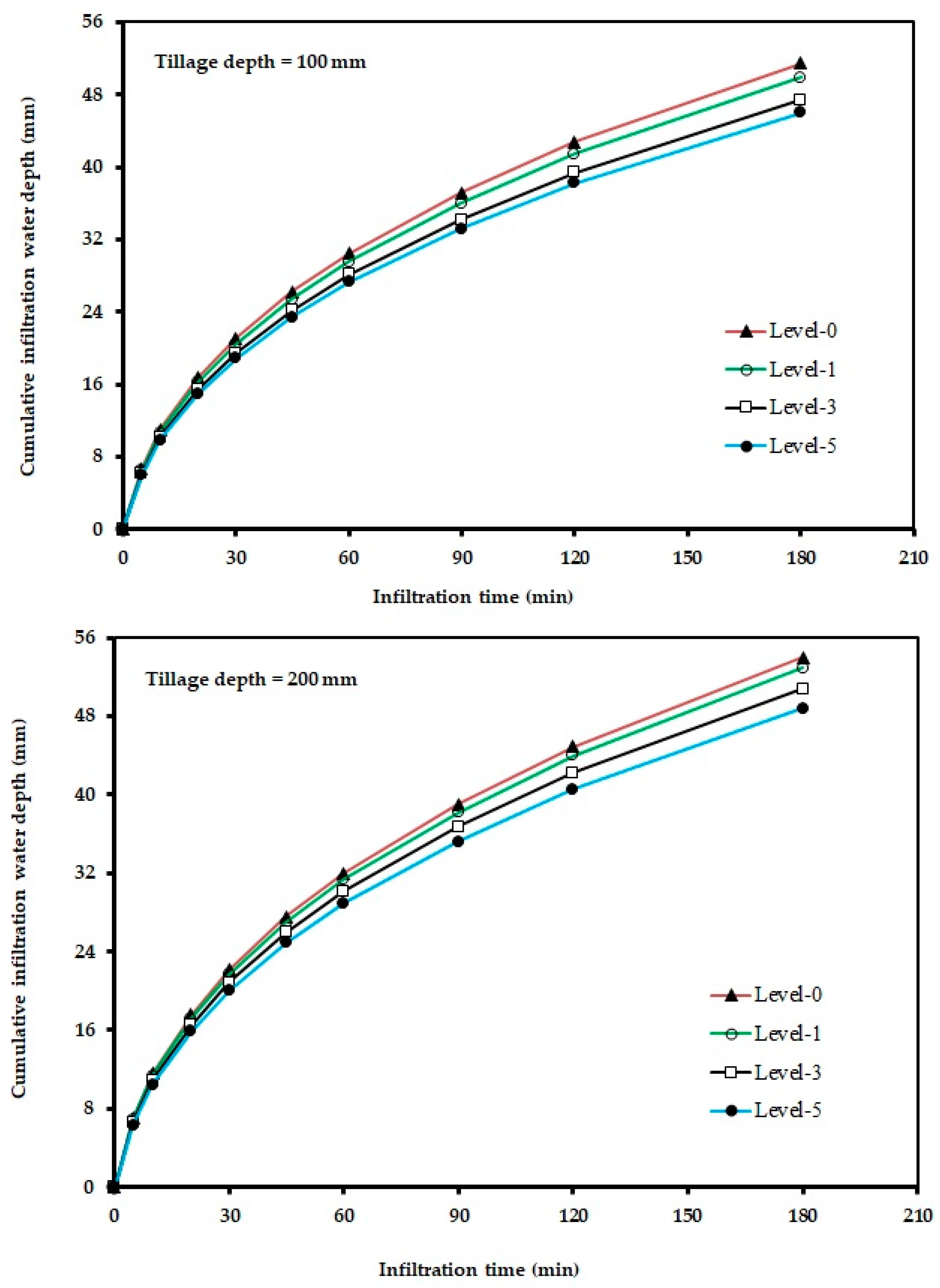
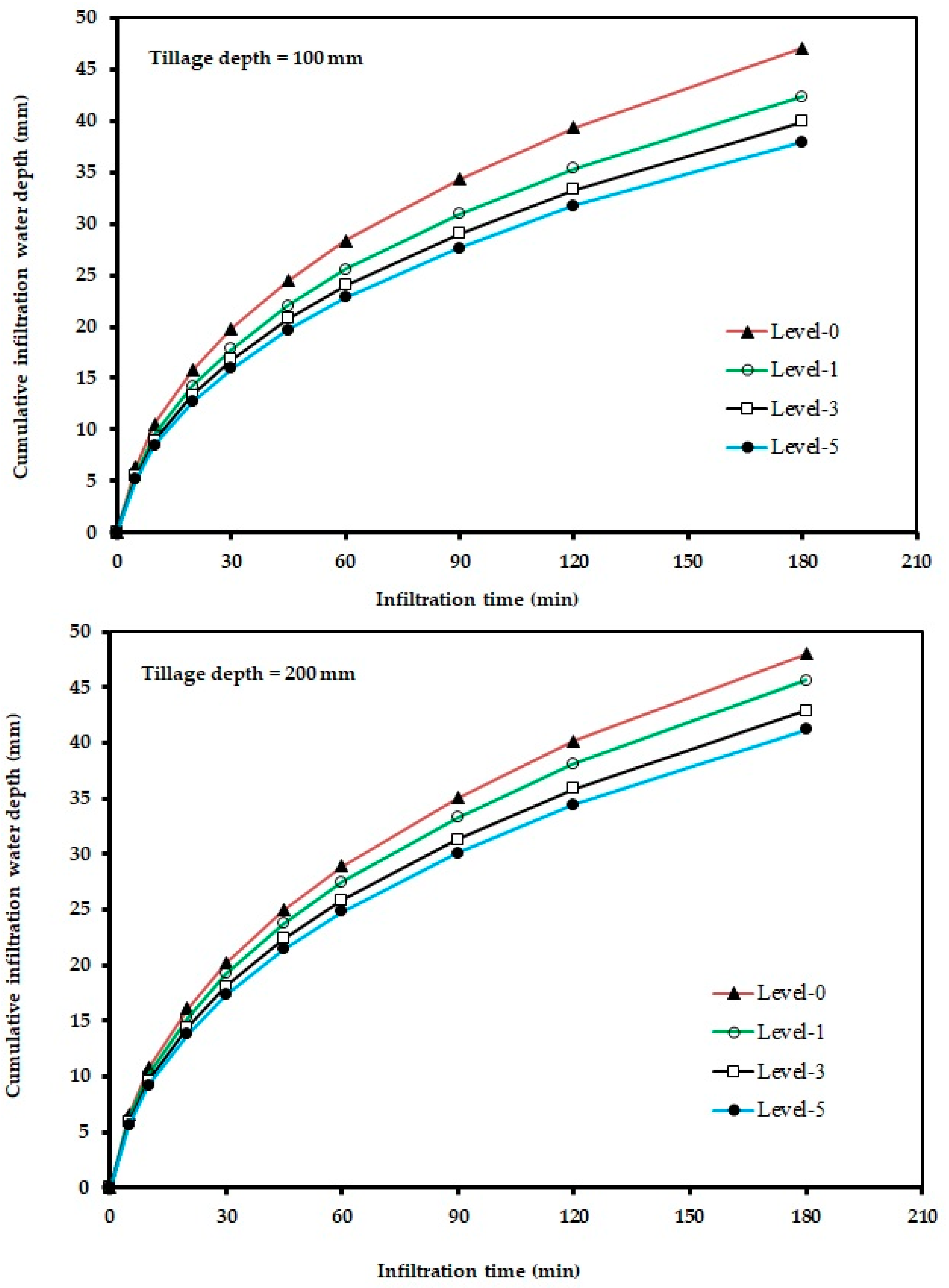
The observed cumulative infiltration depths versus time for the moldboard, chisel and rotary plows are presented in Figure 5, Figure 6 and Figure 7, respectively, under tillage practices with two tillage depths and under different soil compaction levels. Observing Figure 5, Figure 6 and Figure 7, it is clear that the cumulative infiltration generally increases with increasing infiltration time, and it can be expressed as a power function. Figure 8, Figure 9 and Figure 10 present the impact of tillage depth on final cumulative infiltration after 180 min at altered levels of wheel traffic for moldboard, chisel, and rotary plows as average values, respectively. It is noticeable that the water cumulative infiltration depth varied between 46.0 and 54.0 mm after 180 min for the moldboard plow. It varied between 37.9 and 48.0 mm after 180 min for the chisel plow, while for the rotary plow, the cumulative infiltration depth varied between 36.4 and 44.5 mm after 180 min. Water infiltration into the soil is claimed to be directly affected by soil tillage methods [70], and the moldboard plow plot in this research had the ability to take in water at a faster rate than the chisel and rotary plowed plots. This could also be due to the porous nature of the moldboard plow plots and because the soil is coarser than in plots plowed by other tillage implements. The MWD in the moldboard plow plot ranged from 34.5 mm to 80.2 mm; for the chisel plow it ranged from 19.6 mm to 45.7 mm; and for the rotary plow, it ranged from 9.2 mm to 21.5 mm. Generally, primary tillage tends to yield a rough surface finish [71,72]. Plowing processes conducted at different tilling depths and wheel-traffic compaction alter the pore structure of the clay soil [73], and these modifications affect solutes, water movement, and root growth. In a study conducted by Al-Ghazal [74], it was discovered that the chisel plow, followed by the moldboard plow and the rotavator, had the highest mean infiltration rate of soil at the highest rate of compaction (5 passes of the tractor). The additional soil disturbance caused by the chisel plow as compared to moldboard and rotavator plows may be the cause of the higher soil infiltration rate.

3.3. Kostiakov Fitting Parameters

Table 4, Table 5 and Table 6 show the raw data of fitting parameters “q” and “b” in Equation (2) as affected by the number of tractor wheel passes on the plowed soil surface and the tillage depth for the moldboard, chisel, and rotary plows, respectively. Both the estimated Kostiakov fitting parameters, “q” and “b”, obtained by the best fit of measured data differed significantly among the tillage implements (Table 7). Similar results were observed by Mbagwu [75], who reported that the predicted model parameters, “q” and “b”, of the Kostiakov model obtained by the best fit of measured data differed significantly among treatments that included tilled-unmulched, tilled-mulched, untilled-unmulched, untilled-mulched, and continuous pasture. Also, differences cause by wheel traffic were detected in “q” (Table 7). Conversely, there were no significant differences for tillage depth and wheel traffic in “b” and “q” (Table 7). Table 8 presents the mean fitting parameters (Equation (2) as affected by tillage implement, number of wheel traffic passes (soil compaction level), and tillage depth and their interactions.
In this research, the average, maximum and minimum values of “q” were 2.7073, 3.1277, and 2.2724 mm/minb, respectively for a clay soil, and these values were 0.5523, 0.5647, and 0.5424 (dimensionless), respectively, for the “b” parameter for the same clay soil. In another study in a plowed clay, soil “q” was 3.38 mm/minb and “b” was 0.53 (dimensionless) [26]. The infiltration parameters “q” and “b” varied strongly with respect to soil texture [76]. Thus, the Kostiakov model for predicting the water cumulative infiltration (Z, mm) for a clay soil for the present research was as follows:
Z = 2.7073 × t 0.5523 ( Average R 2 was 0.939 )
With an average R2 value of 0.939, only slight variations were reported between the measured and predicted Z. The test results indicate that the cumulative infiltration predicted using Equation (8) is reasonably accurate and can be used to estimate cumulative infiltration over a reasonable time for irrigation in a clay soil. There is a good agreement between the measured and estimated cumulative infiltration under all treatments. In previous research [11], the Kostiakov, Philips, and Horton infiltration models were evaluated and the Kostiakov model was identified as the better alternative for evaluating the infiltration rate. Additionally, the Kostiakov model was considered the most appropriate for the prediction of water infiltration rate into the soil compared with the Horton and Philip models [77]. Fok [78] derived the Kostiakov equation parameters and fitting them to a physically based infiltration equation, derived five different sets of values for “q” and “b”, depending on initial moisture content, time, and hydraulic conductivity. The power constant “b” has more physical sense than the other Kostiakov equation fitting parameters, as its scale depends on the relationships and interactions of several infiltration reduction or increasing factors [78]. According to Dixon [79], large “q” values are related to micro-rough and macro-porous soil surfaces, or to situations with a moderately large gravitational impact on infiltration. On the other hand, small “q” values are linked to smooth, micro-porous surfaces where capillarity is the major force driving infiltration. The constant “b” is just an infiltration curve fitting coefficient. For the empirical infiltration models, it is commonly implicit that, while infiltration is defined as a function of time, the residual parameters are calibration constants signifying the situations under which the test was directed, including the initial soil moisture content and any other factors that may induce differences in infiltration [80].

3.4. Data Analysis of the Third Stage of the Research (Data Mining Algorithms)

Recently, there have been improved research efforts offering alternate approaches for precisely predicting the quantity of soil water infiltration using altered types of models based on data mining models. Some benefits of these kinds of models are reported by Panahi et al. [31] as follows: strong estimation performance, strength in handling missing data, easy and stable to expand, and the ability to handle large quantities of data of diverse measures. The ability of the investigated regression algorithms is reliant upon the default parameters employed by Weka, and the values of the default parameters for the investigated regression algorithms are listed in Table 9. The time taken to build models for “q” and “b” is illustrated in Table 10. The least time is required with the KStar (K*) method. In this research, the input variables were the mean weight diameter, tillage depth and soil compaction level. Various performance measures were used to check the accuracy of the model. The values of “q” and “b” can be computed and compared with actual values of “q” and “b” using the proposed regression models.
The MLP (4-3-1) with three nodes in the hidden layer was formed by Weka. The MLP was trained for 500 epochs with a learning rate of 0.3 and a momentum of 0.2, the Weka defaults. The number of epochs determines how long the MLP will run, while the learning rate and momentum state how in tune the weights are [47]. The Weka linear regression model outcome for “q” was calculated by Equation (8), with an R2 of 0.947, and for “b”, the Weka linear regression model result was calculated by Equation (9), with an R2 of 0.786.
q = 2.2696 + 0.00785 × M W D 0.0171 × N T T + 0.0141 × T D
b = 0.5317 + 0.0004 × M W D + 0.0034 × N T T 0.0002 × T D
where “q” is in mm/mimb, “b” is dimensionless, MWD is in mm, NTT is soil compaction at 0, 1, 3 and 5 traffic levels, and TD is tillage depth in cm.
Table 11 provides the statistical data of the evaluation criteria between the observed and predicted values of the fitting parameters in Equation (2) of “q” and “b” with the investigated regression algorithms. An evaluation of all the regression algorithms was completed to identify the most efficient regression algorithm. Using the testing dataset, the performance of KStar (K*) was better than the other regression algorithms, with the following performance evaluation criteria for “q” estimation: correlation coefficient = 0.997, MAE = 0.0179 mm/minb, and RMSE = 0.0228 mm/minb. For “b” estimation, the performance of the MLP was better than the other regression algorithms, with performance evaluation criteria as follows: correlation coefficient = 0.962, MAE = 0.0013 dimensionless, and RMSE = 0.0026 dimensionless.
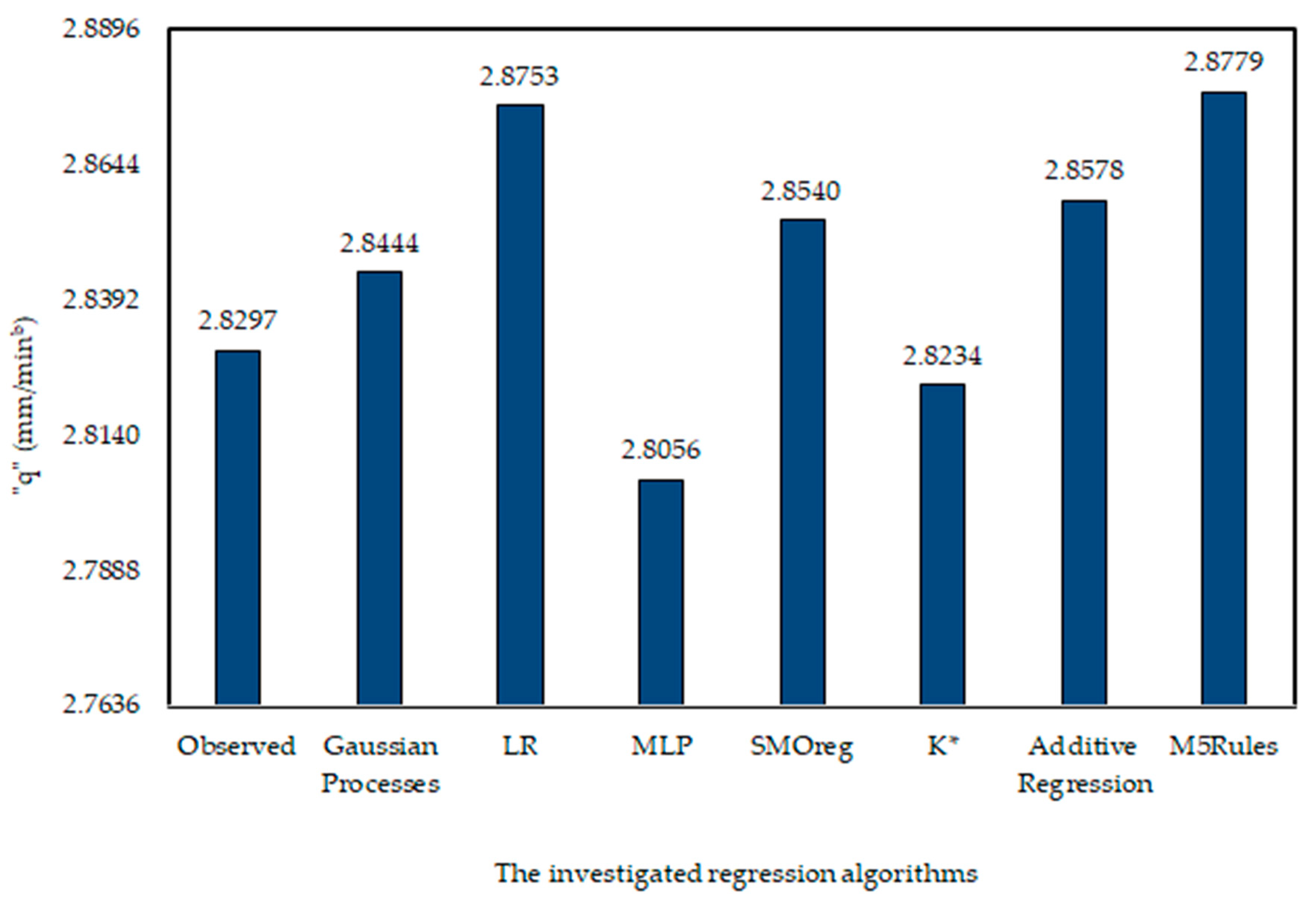
Figure 11 and Figure 12 provide bar graphs for the average values of the parameters of “q” and “b” using the investigated regression algorithms compared with actual values in the testing dataset. The average actual for “b” was 0.5576 dimensionless in the testing dataset (14 points) and the closed average for the KStar (K*) method was 0.5573 dimensionless. The average actual value for “q” was 2.8297 mm/minb in testing dataset (14 points), and the closed average for the K Star (K*) method was 2.8234 mm/minb.
KStar (K*) was the best-performing regression algorithm for predicting the expected values of the parameters “q” and “b” in the used dataset within the studied range. In this case, the K* outcomes were the best for the present dataset, and it is important to note that it is tested here as a regression algorithm and its parameters were left as default in Weka 3.8 software. Furthermore, the KStar algorithm is better than the other prediction regression algorithms, namely, Linear Regression, RBFNetwork, Decision Stump Simple, and Linear Regression in Weka for disorganized data [80]. For prediction of organic matter quantity and clay content in a soil, the Lazy KStar algorithm was shown to have more satisfactory performance when mining the data, with higher determination coefficients and smaller errors [81]. In prediction of rainfall based on metrological data, the KStar algorithm had the maximum correlation coefficient of 0.8901, and the minimum RMSE compared with other algorithms in Weka, including MLP, Bagging, IBk, Additive Regression, Decision Table, Random SubSpace, M5Rules, REPTre, M5P tree, Regression by Discretization, and User Classifier [82]. The efficiency of the deep learning of convolutional neural network (CNN) algorithms, using three metaheuristic procedures for infiltration rate and cumulative infiltration prediction was evaluated. The results revealed that CNN had very good performance for both infiltration rate and cumulative infiltration and prediction [31]. The Kostiakov model, and ANN approach in Weka appeared to be good tools for predicting the infiltration rate of a soil, and time and soil moisture content were the most critical parameters in measurement of the infiltration rate of a soil [83]. In addition, the fitting accuracy of the data mining model is affected by agricultural practices or soil structure, organic matter content, porosity, and other factors [84]. Therefore, this research on the infiltration processes in a clay soil, performed by in situ field observation experiments and fitting a model of infiltration parameters, provides an essential theoretical basis for irrigation management purposes under regular crop production conditions. The research also assists with the selection of the best seedbed preparation method, tillage depth and soil compactions levels generated by tractor passes, enabling the modification of tillage practices during the season to conserve water and to prevent yield declines.

4. Conclusions

To properly plan and manage irrigation systems, cumulative infiltration must be accurately determined. Although infiltration readings frequently only provide point information, they are indispensable for parameter and model validation. This research aimed to investigate in a field experiment the influence on cumulative infiltration of different tillage practices, which were characterized by conducting tillage on a clay soil using three tillage implements (moldboard, chisel, and rotary plows) under two tillage depths and under four levels of soil compaction created by tractor wheel traffic. The analyses indicated that the cumulative infiltration empirical model parameters “q” and “b” of the Kostiakov equation ( Z = q × t b ) depend on the experimental conditions. The logarithmic transformation (graphical method) performance in describing soil infiltration characteristics Z = 2.7073 × t 0.5523 under different tillage practices was tested, resulting in an R2 value of 0.939, and found to be highly acceptable. Defining the precise infiltration features leads to correct management and design of an irrigation system, as governed by the accurate behavior of model parameters. Thus, in this research, regression algorithms in the Weka software, namely, M5Rules, Additive Regression, KStar (K*), SMOreg, Multilayer Perceptron (MLP), Linear Regression (LR), and Gaussian Processes, were used to predict the Kostiakov model parameters of “q” and “b” for the cumulative infiltration equation using field infiltration data. The inputs were as follows: mean weight diameter of the clay soil, which depending on different treatments, ranged from 9.2 to 80.2 mm; the level of tractor wheel traffic on the plowed soil surface (dimensionless) with 0, 1, 3, and 5 passes; and the tillage depth, ranging from 97 to 204 mm. The outputs were “q” and “b”. The obtained results indicated that the KStar (K*) model was the most effective regression algorithm for predicting “q” with a correlation coefficient of 0.997 for the given clay soil texture, while for parameter “b” for the same clay soil texture, the MLP regression algorithm with a correlation coefficient of 0.962 was the most effective method. Finally, we encourage repeating the same procedure in order to answer related problems. This research is not without limitations. Using only the data based on a clay soil is one limitation, although its reliability is high. The second limitation relates to the graphical method for determination of “q” and “b” fitting parameters, as many other methods could have been used, for example, the volume-balance method. The third limitation relates to the non-use of other relevant data mining algorithms that are not offered in Weka software, which should be addressed in coming research on this subject. This research contributes to research in the irrigation field on new computational methods applied to the soil infiltration process. It should encourage the irrigation and soil research community to share their datasets and improve the prediction models. The results also indicate that the regression algorithms can be suitable for the estimation of fitting parameters of cumulative infiltration depth from the accessible data. The fitting parameters generated by the investigated regression algorithms can be used to simulate the cumulative infiltration depth in the investigated soil texture. Moreover, the water infiltration rate into the soil can be used as a tool for the purposes of designing irrigation systems, the characterization of different tillage practices, and providing a localized management of this variable.

Author Contributions

Conceptualization, M.A.-S., R.S.A.-O., S.A.A.-H. and A.M.A.; methodology M.A.-S., A.M.A., R.S.A.-O. and S.A.A.-H.; software, M.A.-S. and A.M.A.; formal analysis, M.A.-S. and A.M.A.; validation, M.A.-S. and S.A.A.-H.; visualization, M.A.-S., R.S.A.-O. and A.M.A.; investigation, M.A.-S. and A.M.A.; resources, M.A.-S. and A.M.A.; data curation, M.A.-S. and A.M.A.; writing—original draft preparation, M.A.-S., A.M.A. and S.A.A.-H.; supervision, M.A.-S., R.S.A.-O. and S.A.A.-H.; funding acquisition, M.A.-S., R.S.A.-O. and A.M.A.; writing—review and editing, all authors. All authors have read and agreed to the published version of the manuscript.

Funding

This research was funded by Researchers Supporting Project (number: RSPD2023R707), King Saud University, Riyadh, Saudi Arabia.

Institutional Review Board Statement

Not applicable.

Informed Consent Statement

Not applicable.

Data Availability Statement

Data are contained within the article.

Acknowledgments

The authors extend their appreciation to the Researchers Supporting Project (number: RSPD2023R707), King Saud University, Riyadh, Saudi Arabia.

Conflicts of Interest

The authors declare no conflict of interest.

References

  1. Mahapatra, S.; Jha, M.K.; Biswal, S.; Senapati, D. Assessing variability of infiltration characteristics and reliability of infiltration models in a tropical sub-humid region of India. Sci. Rep. 2020, 10, 1515. [Google Scholar] [CrossRef] [PubMed] [Green Version]
  2. Fan, Y.; Huang, N.; Gong, J.; Shao, X.; Zhang, J.; Zhao, T. A simplified infiltration model for predicting cumulative infiltration during vertical line source irrigation. Water 2018, 10, 89. [Google Scholar] [CrossRef] [Green Version]
  3. Amami, R.; Ibrahimi, K.; Sher, F.; Milham, P.; Ghazouani, H.; Chehaibi, S.; Hussain, Z.; Iqbal, H.M.N. Impacts of Different tillage practices on soil water infiltration for sustainable agriculture. Sustainability 2021, 13, 3155. [Google Scholar] [CrossRef]
  4. Ahuchaogu, I.I.; Emit, I.; Etuk, A.I. Effects of tillage methods on soil infiltration rate in UYO, Nigeria. Cont. J. Eng. Sci. 2015, 10, 10–20. [Google Scholar]
  5. Villanueva, J.J.M.; García, V.M.V.; Alberich, M.V.E.; Huerta, A.G.; Arriaga, M.R.; Rodríguez, F.G. MEAN infiltration speed in a vertisol under different tillage systems. Terra Latinoam. 2015, 33, 95–99. [Google Scholar]
  6. Osanyinpeju, K.; Dada, P.O. Soil porosity and water infiltration as influenced by tillage practices on federal university of agriculture Abeokuta, Ogun State, Nigeria soil. Int. J. Latest Technol. Eng. Manag. Appl. Sci. 2018, 7, 2278–2540. [Google Scholar]
  7. Atta-Darkwa, T.; Asare, A.; Amponsah, W.; Oppon, E.D.; Agbeshie, A.A.; Budu, M.; Larbi, I.; Akolgo, G.A.; Quaye, D.N.D. Performance evaluation of infiltration models under different tillage operations in a tropical climate. Sci. Afr. 2022, 17, e01318. [Google Scholar] [CrossRef]
  8. Mohammadshirazi, F.; Brown, V.K.; Heitman, J.L.; McLaughlin, R.A. Effects of tillage and compost amendment on infiltration in compacted soils. J. Soil Water Conserv. 2016, 71, 443–449. [Google Scholar] [CrossRef] [Green Version]
  9. Rahman, S.M.; Islam, A. Effects of tillage depth on infiltration characteristics of two Bangladesh soils having plowpans. Soil Tillage Res. 1989, 13, 407–412. [Google Scholar] [CrossRef]
  10. Ibeje, A.O.; Osuagwu, J.C.; Onosakponome, O.R. Impacts of land use on infiltration. World J. Eng. Res. Technol. 2018, 4, 95–102. [Google Scholar]
  11. Dahak, A.; Boutaghane, H.; Merabtene, T. Parameter estimation and assessment of infiltration models for Madjez Ressoul Catchment, Algeria. Water 2022, 14, 1185. [Google Scholar] [CrossRef]
  12. Sajjadi, S.-A.-H.; Mirzaei, M.; Nasab, A.F.; Sarkardeh, H. Effect of soil Physical Properties on infiltration rate. Geomech. Eng. 2016, 10, 727–736. [Google Scholar] [CrossRef]
  13. Mattar, M.A.; Alazba, A.A.; Zin El-Abedin, T.K. Forecasting furrow irrigation infiltration using artificial neural networks. Agric. Water Manag. 2015, 148, 63–71. [Google Scholar] [CrossRef]
  14. Ogbe, V.B.; Jayeoba, O.J.; Ode, S.O. Comparison of four soil infiltration models on a sandy soil in Lafia, Southern Guinea Savanna Zone of Nigeria. PAT 2011, 7, 116–126. [Google Scholar]
  15. Zolfaghari, A.A.; Mirzaee, S.; Gorji, M. Comparison of different models for estimating cumulative infiltration. Int. J. Soil Sci. 2012, 7, 108–115. [Google Scholar] [CrossRef] [Green Version]
  16. Patle, G.T.; Sikar, T.T.; Rawat, K.S.; Singh, S.K. Estimation of infiltration rate from soil properties using regression model for cultivated land. Geol. Ecol. Landsc. 2019, 3, 1–13. [Google Scholar] [CrossRef]
  17. Al-Ghobari, H.M. Modeling soil infiltration under variables of application rate and number of irrigation. J. King Saud Univ. Agric. Sci. 2003, 15, 185–194. [Google Scholar]
  18. Mishra, S.K.; Tyagi, J.V.; Singh, V.P. Comparison of infiltration models. J. Hydrol. Process. 2003, 17, 2629–2652. [Google Scholar] [CrossRef]
  19. Haghiabi, A.H.; Abedi-koupai, J.; Heidarpour, M.; Mohammadzadeh-Habili, J. A new method for estimating the parameters of Kostiakov and modified Kostiakov infiltration equations. World Appl. Sci. J. 2011, 15, 129–135. [Google Scholar]
  20. Adindu, R.U.; Kelechi, K.I.; Chigbu Timothy, O.; Ike-Amadi, C.A. Application of Kostiakov’s infiltration model on the soils of Umudike, Abia State–Nigeria. Am. J. Environ. Eng. 2014, 4, 1–6. [Google Scholar]
  21. Elmarazky, M.S.A.; Aboukarima, A.M.; Guirguis, A.E.; Egela, M.I. Water infiltration as affected by tillage methods, plowing depth and wheel traffic. J. Agric. Sci. Mansoura Univ. 2007, 32, 2019–2033. [Google Scholar]
  22. Hossne García, A.J.; Jesús, M.N.; Smith, I.J.; Velázquez, P.; Leiva, L.M.G.; Gil, A. Effects of compaction, moisture and depth on the parameters of the Kostiakov equation. ESPAMCIENCIA J. 2021, 12, 56–68. [Google Scholar] [CrossRef]
  23. Al-Sulaiman, A.; Aboukarima, A.M.; Zayed, M.F. Prediction of Kostiakov parameters of cumulative infiltration based on soil and water characteristics. Egypt. J. Agric. Res. 2015, 93, 273–291. [Google Scholar]
  24. Sihag, P.; Singh, B.; Sepah, S.A.; Mehdipour, V. Modeling the infiltration process with soft computing techniques. ISH J. Hydraul. Eng. 2018, 26, 138–152. [Google Scholar] [CrossRef]
  25. Sihag, P.; Tiwari, N.K.; Ranjan, S. Support vector regression-based modeling of cumulative infiltration of sandy soil. ISH J. Hydraul. Eng. 2020, 26, 44–50. [Google Scholar] [CrossRef]
  26. Zakwan, M. Assessment of dimensionless form of Kostiakov model. Aquademia: Water Environ. Technol. 2017, 1, 1. [Google Scholar] [CrossRef]
  27. Kashi, H.; Emamqolizadeh, S.; Qorbani, H.; Hashemi, S.A.A. Estimation of soil infiltration using artificial neural network and linear regression in agricultural lands. J. Environ. Eros. Res. 2013, 3, 19–34. [Google Scholar]
  28. Angelaki, A.; Singh, S.; Singh, V.; Sihag, P. Estimation of models for cumulative infiltration of soil using machine-learning methods. ISH J. Hydraul. Eng. 2021, 27, 162–169. [Google Scholar] [CrossRef]
  29. Vand, A.S.; Sihag, P.; Singh, B.; Zand, M. Comparative evaluation of infiltration models. KSCE J. Civ. Eng. 2018, 22, 4173–4184. [Google Scholar] [CrossRef]
  30. Singh, B.; Sihag, P.; Singh, K. Modelling of impact of water quality on infiltration rate of soil by random forest regression. Model. Earth Syst. Environ. 2017, 3, 999–1004. [Google Scholar] [CrossRef]
  31. Panahi, M.; Khosravi, K.; Ahmad, S.; Panahi, S.; Heddam, S.; Melesse, A.; Omidvar, E.; Lee, C. Cumulative infiltration and infiltration rate prediction using optimized deep learning algorithms: A study in Western Iran. J. Hydrol. Reg. Stud. 2021, 35, 100825. [Google Scholar] [CrossRef]
  32. Salifu, A.; Abagale, F.; Kranjac-Berisavljevic, G. Estimation of infiltration models’ parameters using regression analysis in irrigation fields of Northern Ghana. Open J. Soil Sci. 2021, 11, 164–176. [Google Scholar] [CrossRef]
  33. Seongyun, K.; Karahan, G.; Sharma, M.; Pachepsky, Y. Estimating parameters of empirical infiltration models from the global dataset using machine learning. Int. Agrophys. 2021, 35, 73–81. [Google Scholar] [CrossRef]
  34. Tiwari, N.K.; Sihag, P.; Ranjan, S. Modeling of infiltration of soil using adaptive neuro-fuzzy inference system (ANFIS). J. Eng. Technol. Educ. 2017, 11, 13–21. [Google Scholar]
  35. Sayari, S.; Mahdavi-Meymand, A.; Zounemat-Kermani, M. Irrigation water infiltration modeling using machine learning. Comput. Electron. Agric. 2021, 180, 105921. [Google Scholar] [CrossRef]
  36. Voorhees, W.B.; Evans, S.D.; Warnes, D.D. Effect of preplant wheel traffic on soil compaction, water use and growth of spring wheat. Soil Sci. Soc. Am. J. 1985, 49, 215–220. [Google Scholar] [CrossRef]
  37. Li, Y.; Ma, Z.; Liu, Y.; Cui, Z.; Mo, Q.; Zhang, C.; Sheng, H.; Wang, W. Variation in soil aggregate stability due to land use changes from Alpine grassland in a high-altitude watershed. Land 2023, 12, 393. [Google Scholar] [CrossRef]
  38. Kostiakov, A.N. On the dynamics of the coefficient of water percolation in soils and on the necessity of studying it from a dynamic point of view for the purposes of amelioration. Soc. Soil Sci. 1932, 14, 17–21. [Google Scholar]
  39. Uloma, A.R.; Samuel, A.C.; Kingsley, I.K. Estimation of Kostiakov’s infiltration model parameters of some sandy loam soils of Ikwuano–Umuahia. Nigeria. Open Trans. Geosci. 2014, 1, 34–38. [Google Scholar] [CrossRef]
  40. Khaliq, A.; Iqbal, M.; Anwar, S. Evaluation of Kostiakov infiltration equation parameters from irrigation advance in level basins. Pak. J. Agri. Sci. 1994, 31, 258–264. [Google Scholar]
  41. El-Bakhshwan, M.H.; Aboukarima, A.M.; Hemeda, S.G. Impact of mixing biogas liquid manure with soil on water infiltration under flood irrigation system. Asian Res. J. Agric. 2016, 1, 1–12. [Google Scholar] [CrossRef]
  42. Gebl, M.A. Simplified approach for determination of parameters for Kostiakov’s infiltration equation. Water Pract. Technol. 2022, 17, 2435–2446. [Google Scholar] [CrossRef]
  43. Garner, S.R. WEKA: The Waikato Environment for Knowledge Analysis. In Proceedings of the New Zealand Computer Science Research Students Conference; 1995; pp. 57–64. [Google Scholar]
  44. SAS. User’s Guide, Statistical Analysis System; SAS Ins., Inc.: Cary, NC, USA, 1986. [Google Scholar]
  45. Hall, M.; Frank, E.; Holmes, G.; Pfahringer, B.; Reutemann, P.; Ian Witten, H. The WEKA Data Mining Software: An Update. ACM SIGKDD Explor. Newsl. 2009, 11, 10–18. [Google Scholar] [CrossRef]
  46. Frank, E.; Hall, M.; Trigg, L.; Holmes, G.; Witten, I.H. Data mining in bioinformatics using Weka. Bioinformatics 2004, 20, 2475–2481. [Google Scholar] [CrossRef] [PubMed] [Green Version]
  47. Alencar, D.; Carvalho, D.; Koenders, E.; Mourao, F.; Rocha, L. Devising a computational model based on data mining techniques to predict concrete compressive strength. Procedia Comput. Sci. 2017, 108, 455–464. [Google Scholar] [CrossRef]
  48. Cleary, J.G.; Trigg, L.E. k*: An instance-based learner using an entropic distance measure. In Proceedings of the 12th International Conference on Machine Learning, Tahoe City, CA, USA, 9–12 July 1995; pp. 108–114. [Google Scholar]
  49. Wang, K. Introduction to Gaussian Process Regression, Part 1: The Basics. 2022. Available online: https://medium.com/data-science-at-microsoft/introduction-to-gaussian-process-regression-part-1-the-basics-3 (accessed on 8 March 2023).
  50. Shevade, S.; Keerthi, S.; Bhattacharyya, C.; Murthy, K. Improvements to the SMO algorithm for SVM regression. IEEE Trans. Neural Netw. 2000, 11, 1188–1193. [Google Scholar] [CrossRef] [Green Version]
  51. Tso, G.K.; Yau, K.K. Predicting electricity energy consumption: A comparison of regression analysis, decision tree and neural networks. Energy 2007, 32, 1761–1768. [Google Scholar] [CrossRef]
  52. Witten, I.H.; Frank, E. Data Mining: Practical Machine Learning Tools and Techniques; Morgan Kaufmann Pub: Cambridge, MA, USA, 2005. [Google Scholar]
  53. Wormstrand, O. Electricity Price Prediction. A Comparison of Machine Learning Algorithms. Master’s Thesis, Ostfold University College, Halden, Norway, 2011. [Google Scholar]
  54. Haykin, S. Neural Networks: A Comprehensive Foundation, 2nd ed.; Prentice-Hall: Upper Saddle River, NJ, USA, 1999. [Google Scholar]
  55. Chaudhari, M.S.; Choudhari, N.K. Study of various rainfall estimation & prediction techniques using data mining. Am. J. Eng. Res. (AJER) 2017, 6, 137–139. [Google Scholar]
  56. Brouwer, C.; Goffeau, A.; Heibloem, M. Irrigation Water Management: Training Manual No. 1-Introduction to Irrigation. FAO—Food and Agriculture Organization of the United Nations. 1985. Available online: http://www.fao.org/docrep/r4082e/r4082e00.htm#Contents (accessed on 1 April 2023).
  57. Romkens, M.J.; Luk, M.S.H.; Poesen, J.W.A.; Mermut, A.R. Rainfall infiltration into loess soils from different geographic regions. Catena 1995, 25, 21–32. [Google Scholar] [CrossRef]
  58. Hwang, S.I.; Powers, S.E. Using particle-size distribution models to estimate soil hydraulic properties. Soil Sci. Soc. Am. 2003, 67, 1103–1112. [Google Scholar] [CrossRef]
  59. Hamza, M.A.; Anderson, W.K. Soil compaction in cropping systems: A review of the nature, causes, and possible solutions. Soil Tillage Res. 2005, 82, 121–145. [Google Scholar] [CrossRef]
  60. Khadr, K.A. Effect of some primary tillage implement on soil pulverization and specific energy. Misr. J. Agric. Eng. 2008, 25, 731–745. [Google Scholar] [CrossRef]
  61. Hajabbasi, M.A.; Hemmat, A. Tillage impacts on aggregate stability and crop productivity in a clay-loam soil in central Iran. Soil Tillage Res. 2000, 56, 205–212. [Google Scholar] [CrossRef]
  62. Çarman, K. Effect of different tillage systems on soil properties and wheat yield in middle Anatolia. Soil Tillage Res. 1997, 40, 201–207. [Google Scholar] [CrossRef]
  63. Boydas, M.G.; Turgut, N. Effect of tillage implements and operating speeds on soil physical properties and wheat emergence. Turk. J. Agric. For. 2007, 31, 399–412. [Google Scholar]
  64. Carter, M.R. Characterization of soil physical properties and organic matter under long-term primary tillage in a humid climate. Soil Tillage Res. 1996, 38, 251–263. [Google Scholar] [CrossRef]
  65. Naseer, S.; Kadhim, A.; Subr, K. Effect of tillage with chisel plow on soil mean weight diameter and porosity. Iraqi J. Agric. Sci. 2012, 33, 33–41. [Google Scholar]
  66. Yassen, H.A.; Hassan, H.M.; Hammadi, I.A. Effects of plowing depth using different plow types on some physical properties of soil. AMA 1992, 23, 21–24. [Google Scholar]
  67. Ramezani, N.; Sayyad, G.A.; Barzegar, A.R. Tractor wheel compaction effect on soil water infiltration, hydraulic conductivity and bulk density. Malays. J. Soil Sci. 2017, 21, 47–61. [Google Scholar]
  68. Barzegar, A.R.; Hashemi, A.M.; Herbert, S.J.; Asoodar, M.A. Interactive effects of tillage system and soil water content on aggregate size distribution for seedbed preparation in Fluvisols in southwest Iran. Soil Tillage Res. 2004, 78, 45–52. [Google Scholar] [CrossRef]
  69. Yadav, R.K.; Singh, P.; Singh, S.K. Performance analysis of rotavator and other tillage implement driven by the tractor. Int. J. Agric. Eng. 2017, 10, 590–594. [Google Scholar] [CrossRef]
  70. Moret, D.; Arrué, J.L. Characterizing soil water-conducting macro- and mesoporosity as influenced by tillage using tension infiltrometry. Soil Sci. Soc. Am. J. 2007, 71, 500–506. [Google Scholar] [CrossRef] [Green Version]
  71. Flowers, M.D.; Lal, R. Axle load and tillage effects on soil physical properties and soybean grain yield on a Mollic ochraqualf in Northwest Ohio. Soil Tillage Res. 1998, 48, 21–35. [Google Scholar] [CrossRef]
  72. Reicosky, D.C. Long term effect of moldboard plowing on tillage induced CO2 loss. In Agricultural Practices and Policies for Carbon Sequestration in Soil; Kimble, J.M., Lal, R., Follet, R.F., Eds.; CRC/Lewis: Boca Raton, FL, USA, 2002; pp. 87–97. [Google Scholar]
  73. Ankeny, M.D.; Kaspar, T.C.; Horton, R. Characterization of tillage and traffic effects on unconfined infiltration measurements. Soil Sci. Soc. Am. J. 1990, 54, 837–840. [Google Scholar] [CrossRef] [Green Version]
  74. Al-Ghazal, A.A. Effect of tillage practices and compaction on infiltration rate of sandy soils. Pak. J. Biol. Sci. 2000, 3, 1443–1446. [Google Scholar] [CrossRef] [Green Version]
  75. Mbagwu, J.S.C. Testing the goodness of fit of infiltration models for highly permeable soils under different tropical soil management systems. Soil Tillage Res. 1995, 34, 199–205. [Google Scholar] [CrossRef]
  76. Al-Matroud, S.S. Evaluation of Irrigation Water Quality and its Effect on Soil Infiltration Rate in Riyadh Region. Master’s Thesis, College of Agriculture, King Saud University, Riyadh, Saudi Arabia, 2003. (In Arabic). [Google Scholar]
  77. Eze, P.C.; Musa, J.J. Prediction of infiltration rates of fallow and cultivated soils in Minna, Southern Guinea Savanna zone of Nigeria. J. Soil Water Conserv. 2022, 21, 337–344. [Google Scholar] [CrossRef]
  78. Fok, Y.-S. Derivation of Lewis-Kostiakov intake equation. J. Irrig. Drain. Eng. 1986, 112, 164–171. [Google Scholar] [CrossRef]
  79. Dixon, R.M.; Simanton, J.R.; Lane, L.J. Simple Time-Power Functions for Rainwater Infiltration and Runoff. Arizona-Nevada Academy of Science. 1978. Available online: http://hdl.handle.net/10150/301042 (accessed on 1 April 2023).
  80. Guzmán-Rojo, D.B.; Bautista, E.; Gonzalez-Trinidad, J.; Bronson, K.F. Variability of furrow infiltration and estimated infiltration parameters in a macroporous soil. J. Irrig. Drain. Eng. 2019, 145, 16. [Google Scholar] [CrossRef] [Green Version]
  81. Teixeira, S.; Guimarães, A.M.; Proença, C.A.; da Rocha, J.C.F.; Caires, E.F. Data mining algorithms for prediction of soil organic matter and clay based on Vis-NIR Spectroscopy. Int. J. Agric. For. 2014, 4, 310–316. [Google Scholar]
  82. Bushara, N.O.; Abraham, A. Weather forecasting in Sudan using machine learning schemes. J. Netw. Innov. Comput. 2014, 2, 309–317. [Google Scholar]
  83. Sihag, P.; Singh, S. Modeling of Infiltration Rate Using Data Mining Models. Conference Paper (I-CONCEPTS-18/). 2018. Available online: http://www.gjesr.com/Issues%20PDF/I-CONCEPTS-18/32.pdf (accessed on 10 March 2023).
  84. Khasraei, A.; Abyaneh, H.Z.; Jovzi, M.; Albaji, M. Determining the accuracy of different water infiltration models in lands under wheat and bean cultivation. J. Hydrol. 2021, 603, 127122. [Google Scholar] [CrossRef]
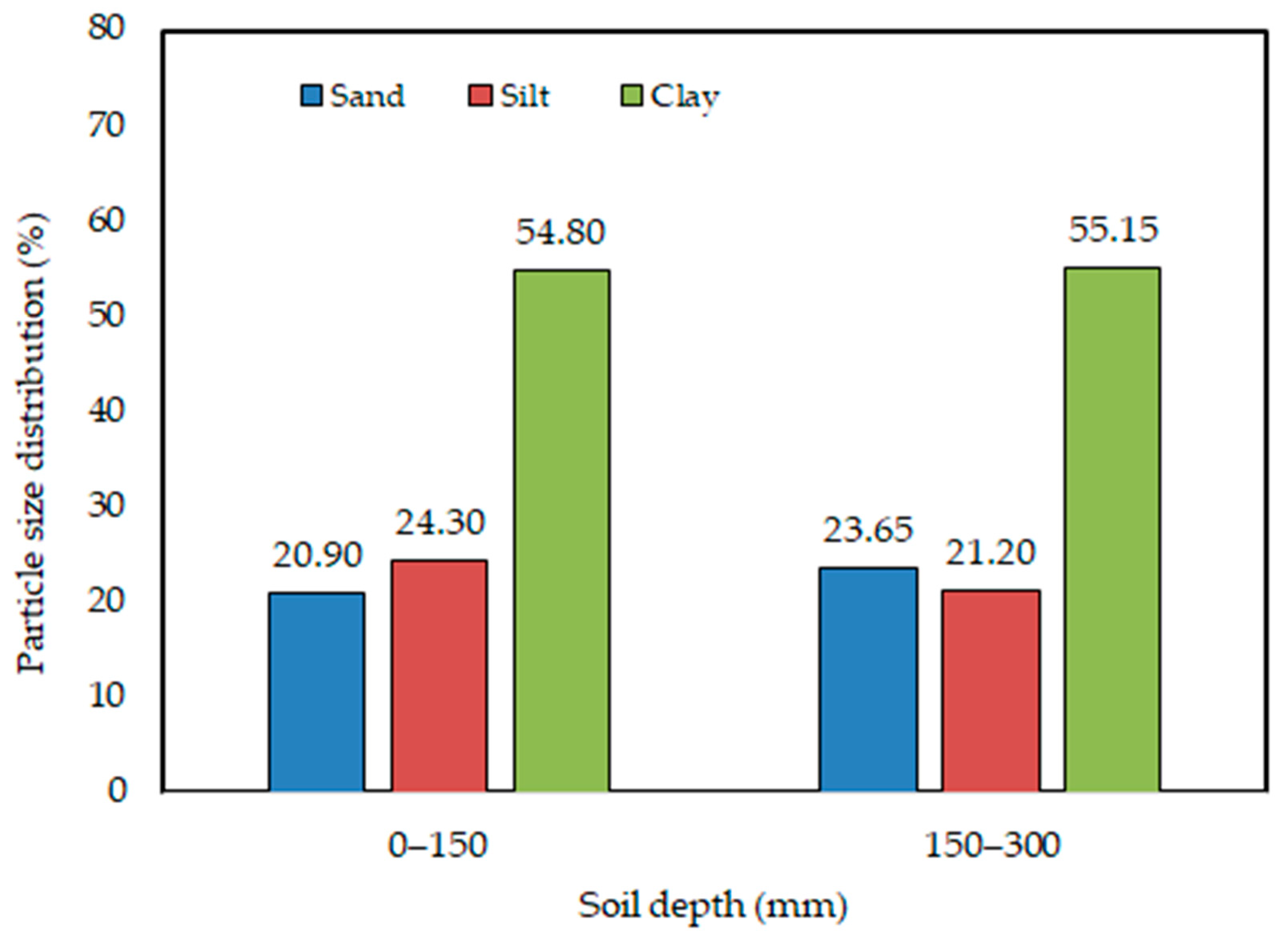
Figure 1. Average percentage of silt, clay, and sand content at the experimental location for two soil depths.
Water 15 02673 g001
Figure 2. Steps of the research methodology used to obtain the parameters “q” and “b” (adopted from [42]).
Water 15 02673 g002
Figure 3. Flowchart for modeling of “q” and “b” in Equation (2) using Weka software.
Water 15 02673 g003
Figure 4. Variation in average soil MWD under investigated tillage practices treatments for rotary, chisel, and moldboard plows (D1 represents a tillage depth of 100 mm and D2 represents a tillage depth of 200 mm).
Water 15 02673 g004
Figure 5. Field measurements of cumulative infiltration depths for moldboard plow tillage with two tillage depths and under different soil compaction levels.
Water 15 02673 g005
Figure 6. Field measurements of cumulative infiltration depths for chisel plow tillage with two tillage depths and under different soil compaction levels.
Water 15 02673 g006
Figure 7. Field measurements of cumulative infiltration depths for rotary plow tillage with two tillage depths and under different soil compaction levels.
Water 15 02673 g007
Figure 8. Impact of tillage depth on final water cumulative infiltration depth after 180 min at different levels of wheel traffic for moldboard plow. Data are shown as average values.
Water 15 02673 g008
Figure 9. Impact of tillage depth on final water cumulative infiltration depth after 180 min at different levels of wheel traffic for chisel plow. Data are shown as average values.
Water 15 02673 g009
Figure 10. Impact of tillage depth on final water cumulative infiltration depth after 180 min at different levels of wheel traffic for rotary plow. Data are shown as average values.
Water 15 02673 g010
Figure 11. Bar graph for the average values of the parameter “q” using the investigated regression algorithms compared with actual values in testing dataset.
Water 15 02673 g011
Figure 12. Bar graph for the average values of the parameter “b” using the investigated regression algorithms compared with observed values in testing dataset.
Water 15 02673 g012
Table 1. Descriptions of Weka regression algorithms.
ClassAlgorithmsDescription
RuleM5RulesBy using separate-and-conquer, this generates a decision list for regression issues. It employs M5 to construct a model tree in each cycle, turning the “best” leaf into a rule [47].
MetaAdditive RegressionA fitting model’s residuals are adjusted interactively for prediction while taking earlier iterations into account [47].
LazyKStar (K*)An entropy-based distance function is used to calculate how similar the training examples are in order to make predictions [48].
FunctionGaussian ProcessesRegression without hyper-parameter tweaking is performed. This measures the match between arguments to forecast the value using lazy learning [49].
SMOregThe algorithm is dependent on the support vector machine method for regression predictions [50].
Table 2. Analysis of variance (ANOVA) table of the MWD (TI indicates tillage implement, NTT indicates the number of tractor wheel traffic passes on the plowed soil surface, and TD indicates the tillage depth).
Source of VariationDegrees of FreedomAnova SSMean SquareF-Valuep-Values
Replicates22.451.24.530.0160
TI221,752.610,876.340,159.1<0.0001
NTT36587.72195.98108.07<0.0001
TD1168.2168.2621.01<0.0001
T I × N T T 61583.9263.9974.70<0.0001
T I × T D 240.420.274.65<0.0001
N T T × T D 31.30.441.640.1942
T I × N T T × T D 60.320.0530.200.9762
Table 3. Mean values and least significance difference (LSD) for the MWD as impacted by tillage implement, soil compaction level, and tillage depth (Means significantly different if they are followed by a distinct letter).
TreatmentsMean MWD (mm)
Moldboard plow57.86 a
Chisel plow32.98 b
Rotary plow15.50 c
LSD (5%)0.30
Soil compaction level-047.84 a
Soil compaction level-140.67 b
Soil compaction level-330.52 c
Soil compaction level-522.76 d
LSD (5%)0.35
Tillage depth (100 mm)33.92 b
Tillage depth (200 mm)36.98 a
LSD (5%)0.25
Table 4. Raw data of fitting parameters “q” and “b” in Equation (2) as affected by the number of tractor wheel passes on the plowed soil surface and the tillage depth for the moldboard plow.
Soil MWD (mm)Number of Tractor Wheel Passes on the Plowed Soil Surface (-)Tillage Depth (mm)Replicates“q” (mm/minb)“b”
(Dimensionless)
75.50104R12.9790.5595
77.60108R22.9630.5637
74.80103R32.9620.5634
80.40189R13.1280.5595
79.70201R23.1240.5627
80.50197R33.1190.5627
63.41105R12.8890.5595
65.2198R22.8880.5627
62.81106R32.8790.5627
69.11198R13.0650.5595
68.51204R23.0510.5631
69.21189R33.0630.5624
46.93102R12.7450.5595
48.23104R22.7350.5627
46.53105R32.7380.5636
52.53194R12.9430.5595
52.13198R22.9260.5640
52.63189R32.9410.5621
34.3598R12.6630.5595
35.2597R22.6510.5632
33.95108R32.6420.5647
39.95198R12.8250.5595
39.65194R22.8010.5647
40.05197R32.8180.5625
Table 5. Raw data of fitting parameters “q” and “b” in Equation (2) as affected by the number of tractor wheel passes on the plowed soil surface and the tillage depth for the chisel plow.
Soil MWD (mm)Number of Tractor Wheel Passes on the Plowed Soil Surface (-)Tillage Depth (mm)Replicates“q” (mm/minb)“b”
(Dimensionless)
43.00104R12.9180.546
44.20107R22.9000.551
42.60106R32.9000.551
45.80195R12.9760.546
45.40203R22.9710.550
45.90198R32.9660.550
36.11107R12.6260.546
37.21102R22.6230.550
35.81114R32.6150.550
39.41207R12.8270.546
39.11197R22.8120.551
39.51207R32.8240.550
26.83104R12.4690.546
27.53103R22.4570.550
26.5398R32.4600.551
30.03187R12.6580.546
29.73197R22.6390.552
30.03198R32.6550.550
19.55102R12.3450.546
20.1599R22.3320.551
19.35108R32.3220.553
22.85201R12.5510.546
22.65194R22.5260.553
22.85198R32.5430.550
Table 6. Raw data of fitting parameters “q” and “b” in Equation (2) as affected by the number of tractor wheel passes on the plowed soil surface and the tillage depth for the rotary plow.
Soil MWD (mm)Number of Tractor Wheel Passes on the Plowed Soil Surface (-)Tillage Depth (mm)Replicates“q” (mm/minb)“b”
(Dimensionless)
20.2098R12.6790.5424
20.80104R22.6600.5475
20.00103R32.6600.5471
21.50195R12.8130.5424
21.40198R22.8080.5464
21.60198R32.8030.5463
17.01104R12.5990.5424
17.51111R22.5950.5464
16.81109R32.5870.5463
18.51198R12.7010.5424
18.41196R22.6840.5469
18.51198R32.6960.5461
12.6397R12.4690.5424
12.9398R22.4570.5463
12.5397R32.4600.5475
14.13197R12.5930.5424
14.03195R22.5740.5480
14.13189R32.5890.5457
9.25104R12.2960.5424
9.4598R22.2830.5471
9.15108R32.2720.5490
10.75198R12.4110.5424
10.65187R22.3850.5491
10.75187R32.4020.5463
Table 7. Source of variation, degrees of freedom (DF) and probability (p-values) from ANOVA table for e fitting parameters “q” and “b” in Equation (2).
Source of VariationDFp-Values
“q” (mm/minb)“b” (Dimensionless)
TI2<0.0001<0.0001
NTT30.01520.9868
TD10.09020.2770
T I × N T T 60.99501.000
T I × T D 20.97140.9954
N T T × T D 30.99670.9355
T I × N T T × T D 61.00001.000
Table 8. Mean fitting parameters (Equation (2)), as affected by tillage implements, number of wheel passes (soil compaction level) and tillage depths, and least significance difference (LSD) (Means are significantly different if they are followed by a distinct letter).
TreatmentsMean Fitting Parameters
“q” (mm/minb)“b” (Dimensionless)
Moldboard plow2.89736 a0.5619581 a
Chisel plow2.66316 b 0.5493522 b
Rotary plow2.56147 c0.5454777 c
LSD (5%)0.07820.0015
Soil compaction level-02.78313 a0.5521947 a
Soil compaction level-12.73002 ba0.5521412 a
Soil compaction level-32.67475 b0.5522829 a
Soil compaction level-52.64142 b0.5524318 a
LSD (5%)0.09030.0017
Tillage depth (200 mm)2.73479 a0.5525892 a
Tillage depth (100 mm)2.67987 a0.5519362 a
LSD (5%)0.06390.0012
Table 9. Default WEKA information for investigated models.
Regression AlgorithmWEKA Information
M5RulesScheme: weka.classifiers.rules.M5Rules -M 4.0
Additive RegressionScheme: weka.classifiers.meta.AdditiveRegression -S 1.0 -I 10 -W weka.classifiers.trees.DecisionStump
KStar (K*)Scheme: weka.classifiers.lazy.KStar -B 20 -M a
Gaussian ProcessesScheme: weka.classifiers.functions.GaussianProcesses -L 1.0 -N 0 -K “weka.classifiers.functions.supportVector.RBFKernel -C 250007 -G 1.0”
SMOregScheme: weka.classifiers.functions.SMOreg -C 1.0 -N 0 -I “weka.classifiers.functions.supportVector.RegSMOImproved -L 0.001 -W 1 -P 1.0E-12 -T 0.001 -V” -K “weka.classifiers.functions.supportVector.PolyKernel -C 250007 -E 1.0”
LRScheme: weka.classifiers.functions.LinearRegression -S 0 -R 1.0E-8
MLPScheme: weka.classifiers.functions.MultilayerPerceptron -L 0.3 -M 0.2 -N 500 -V 0 -S 0 -E 20 -H a
Table 10. Time taken (s) to build model in seconds for fitting parameters of “q” and “b”.
Regression Algorithm“q” (mm/minb)“b” (Dimensionless)
Gaussian Processes1.601.62
Linear Regression0.010.01
Multilayer Perceptron0.150.17
SMOreg0.010.04
KStar (K*)0.000.00
Additive Regression0.030.02
M5Rules0.250.25
Table 11. The statistical data of evaluation criteria between actual and predicted values of the fitting parameters of “q” and “b” in Equation (2) using different regression algorithms using testing dataset.
Regression Algorithm“q” (mm/minb)“b” (Dimensionless)
MAERMSECorrelation CoefficientMAERMSECorrelation Coefficient
M5Rules0.05750.07020.9460.00210.00280.808
Additive Regression0.04590.06380.9260.00260.00420.564
KStar (K*) 0.01790.02280.9970.00210.00270.805
SMOreg0.03730.07710.9480.00190.00260.828
Multilayer Perceptron (MLP)0.04250.09100.9510.00130.00260.962
Linear Regression (LR)0.05440.06670.9470.00230.00290.786
Gaussian Processes0.06040.08170.9590.00330.00420.711
Disclaimer/Publisher’s Note: The statements, opinions and data contained in all publications are solely those of the individual author(s) and contributor(s) and not of MDPI and/or the editor(s). MDPI and/or the editor(s) disclaim responsibility for any injury to people or property resulting from any ideas, methods, instructions or products referred to in the content.