A Large-Scale Group Decision-Making Approach to Assess Water Resource Sustainability with Double-Level Linguistic Preference Relation


Abstract
:1. Introduction
2. Preliminaries
2.1. HLTS and DHLTS
2.2. Minority Opinions and Non-Cooperative Behavior
2.3. DLLPR
- (1)
- Elements on the diagonal of the matrix ;
- (2)
- If , then the element is in its symmetric position .
- (1)
- ;
- (2)
- .
3. Clustering, Weight Calculation, and Consensus Level Determination Methods
3.1. Key Information on the LGWRSA Issue of DLLPR
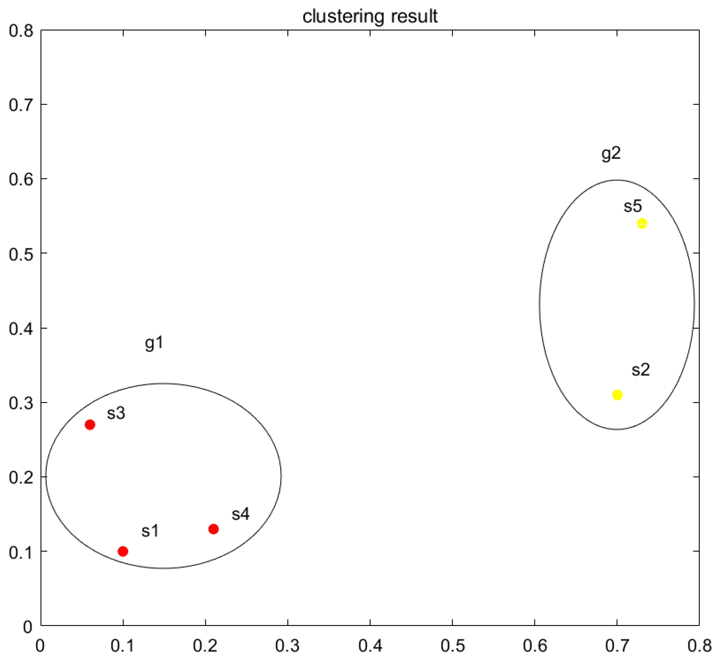
3.2. Clustering Method Based on DLLPR
3.3. Weight Determination Method
4. Consensus Reaching Process and Scoring Calculation
4.1. Comprehensive Adjustment Factor
- A.
- Subjective adjustment factor:
- B.
- Objective adjustment factor:
- C.
- Comprehensive adjustment factor:
4.2. Managing Minority Opinions
- A.
- Identify minority views
- (1)
- The subgroup should have the least degree of consensus
- (2)
- The number of members in this subgroup is less than the average number of members per subgroup.
- B.
- Judge whether the opinion of this subgroup is worth adopting
- C.
- Adjust the weight of this minority subgroup
4.3. Dealing with Non-Cooperative Behavior
- A.
- Identify non-cooperative groups:
- B.
- Measure the degree of non-cooperation:
- C.
- Adjust the weight of non-cooperative groups:
- (1)
- If , then the subgroup can be considered as a fully cooperative group. There is no need to change the weight of ; directly use the comprehensive adjustment coefficient to adjust their preferences;
- (2)
- If , then the subgroup can be considered as a completely uncooperative group. The extreme opinions of this subgroup do not have any positive impact on our decision making, so the best choice is to delete them;
- (3)
- If , then the subgroup can be considered as a partially uncooperative group. Therefore, it should adjust their weights to improve their opinions and then use the comprehensive adjustment coefficient to adjust their preferences.
4.4. Scoring Calculation
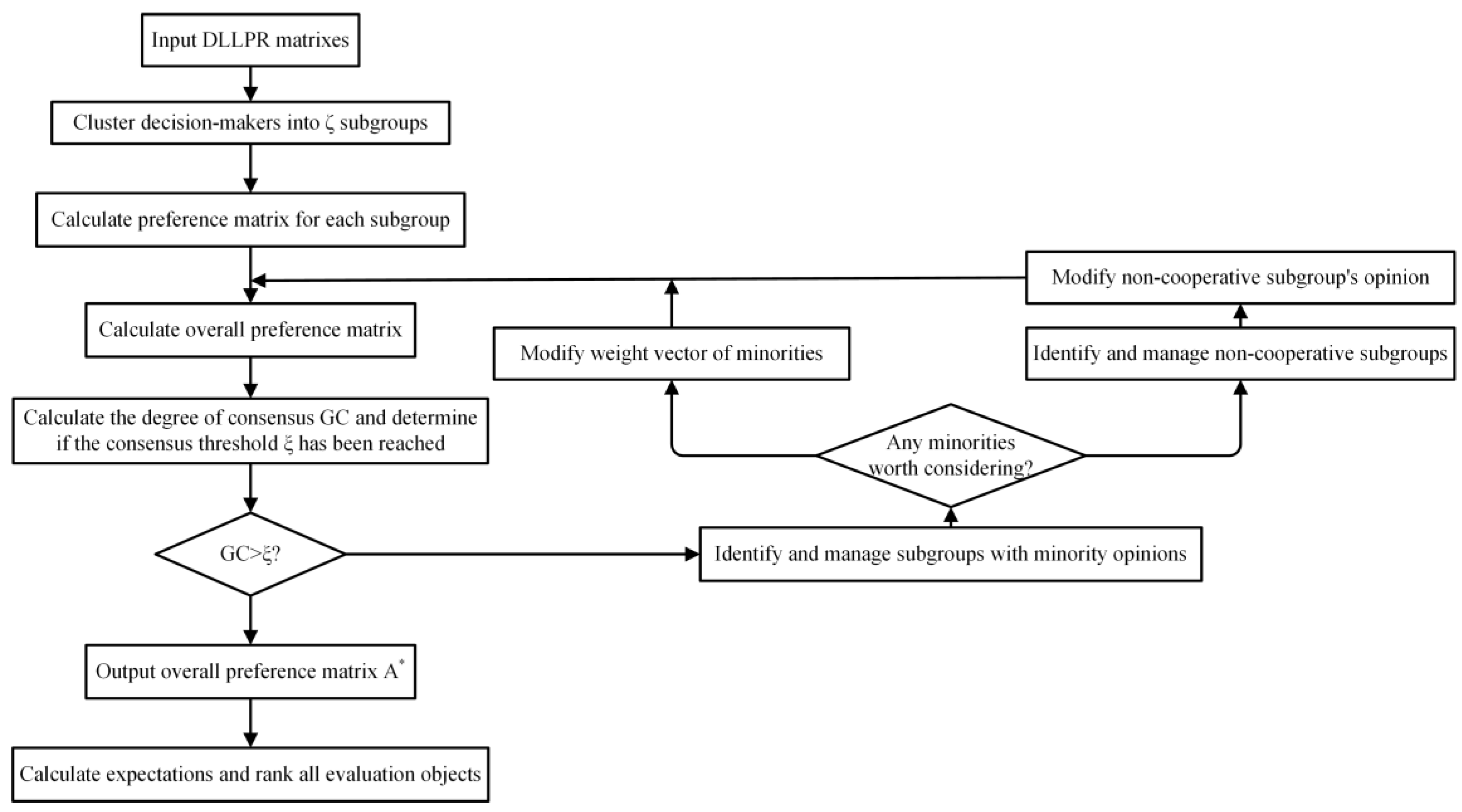
4.5. Summarize this Algorithm
5. Case Study
5.1. Subjective Assessment Results
5.2. Overall Assessment Results
6. Discussion
6.1. Analyzing the Results of the Case Study
6.2. Comparative Analysis
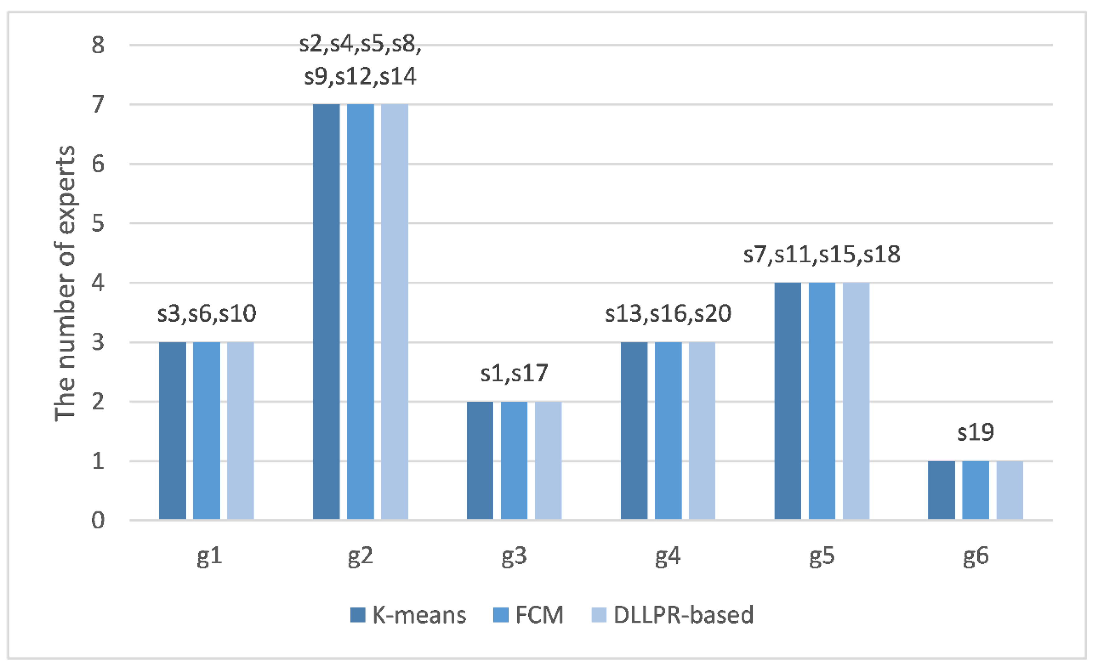
6.3. Comparative Experiments for the Clustering
7. Conclusions
Author Contributions
Funding
Conflicts of Interest
Abbreviations
| LGWRSA | Large-scale group water resource sustainability assessment |
| DLLPR | Double-level linguistic preference relation |
| MCDM | Multi-criteria decision making |
| FCM | Fuzzy c-Method |
| CRP | Consensus building process |
| CAP | Clustering analysis progress |
| HFLTS | Hesitant fuzzy linguistic term set |
| DHLTS | Double hierarchy linguistic term set |
| m | Number of experts |
| n | Number of objects the expert evaluates |
| ω | The weight of experts/subgroups |
| C | Consistency |
| GC | Global consistency |
| ξ | Consensus threshold |
| gλ | Subgroup λ |
| εgλ | Comprehensive adjustment factor |
| εsgλ | Subjective adjustment factor |
| εogλ | Objective adjustment factor |
| ∆λ | Weight adjustment coefficient of gλ |
| ψλ | The degree of non-cooperation |
References
- Li, Z.; Zhang, Q.; Liao, H. Efficient-equitable-ecological evaluation of regional water resource coordination considering both visible and virtual water. Omega Int. J. Manag. Sci. 2019, 83, 223–235. [Google Scholar] [CrossRef]
- Wang, Q.; Li, S.; Li, R. Evaluating water resource sustainability in Beijing, China: Combining PSR model and matter-element extension method. J. Clean. Prod. 2019, 206, 171–179. [Google Scholar] [CrossRef]
- Dong, H.; Feng, Z.; Yang, Y. Sustainability assessment of critical natural capital: A case study of water resources in Qinghai Province, China. J. Clean. Prod. 2021, 286, 125532. [Google Scholar] [CrossRef]
- Dehkordi, M.A.; Haddad, O.B.; Chu, X. Development of a Combined Index to Evaluate Sustainability of Water Resources Systems. Water Resour. Manag. 2021, 35, 2965–2985. [Google Scholar] [CrossRef]
- Zheng, C.L.; Zhou, Y.Y.; Zhou, L.G. Clustering and compatibility-based approach for large-scale group decision making with hesitant fuzzy linguistic preference relations: An application in e-waste recycling. Expert Syst. Appl. 2022, 197, 116615. [Google Scholar] [CrossRef]
- Zhou, S.J.; Zhou, J.X.; Chen, S.C. Outlier identification and group satisfaction of rating experts: Density-based spatial clustering of applications with noise based on multi-objective large-scale group decision-making evaluation. Econ. Res. Ekon. Istraz. 2023, 36, 562–592. [Google Scholar] [CrossRef]
- Yang, M.S.; Lin, C.Y. Block Fuzzy K-modes Clustering Algorithm. In Proceedings of the 18th IEEE International Conference on Fuzzy Systems, Jeju, Republic of Korea, 20–24 August 2009; pp. 384–389. [Google Scholar]
- Rodríguez, R.M.; Martinez, L.; De Tré, G. A consensus model for large scale using hesitant information. In Proceedings of the 13th International FLINS Conference (FLINS 2018), Belfast, UK, 21–24 August 2018; pp. 198–204. [Google Scholar]
- Liu, X.; Xu, Y.; Montes, R.; Ding, R.X.; Herrera, F. Alternative ranking-based clustering and reliability index-based consensus reaching process for hesitant fuzzy large scale group decision making. IEEE Trans. Fuzzy Syst. 2018, 27, 159–171. [Google Scholar] [CrossRef]
- Li, S.L.; Wei, C.P. A two-stage dynamic influence model-achieving decision-making consensus within large scale groups operating with incomplete information. Knowl.-Based Syst. 2020, 189, 105132. [Google Scholar] [CrossRef]
- Gao, P.Q.; Huang, J.; Xu, Y.J. A k-core decomposition-based opinion leaders identifying method and clustering-based consensus model for large-scale group decision making. Comput. Ind. Eng. 2020, 150, 106842. [Google Scholar] [CrossRef]
- Rodríguez, R.M.; Labella, A.; Sesma-Sara, M.; Bustince, H.; Martínez, L. A cohesion-driven consensus reaching process for large scale group decision making under a hesitant fuzzy linguistic term sets environment. Comput. Ind. Eng. 2021, 155, 107158. [Google Scholar] [CrossRef]
- Wu, T.; Liu, X.W.; Qin, J.D.; Herrera, F. Balance Dynamic Clustering Analysis and Consensus Reaching Process With Consensus Evolution Networks in Large-Scale Group Decision Making. IEEE Trans. Fuzzy Syst. 2021, 29, 357–371. [Google Scholar] [CrossRef]
- Rodríguez, R.M.; Liu, H.; Martínez, L. A Fuzzy Representation for the Semantics of Hesitant Fuzzy Linguistic Term Sets. In Foundations of Intelligent Systems; Wen, Z., Li, T., Eds.; Springer: Berlin/Heidelberg, Germany, 2014; Volume 277. [Google Scholar]
- Gou, X.J.; Xu, Z.S. Double hierarchy linguistic term set and its extensions: The state-of-the-art survey. Int. J. Intell. Syst. 2021, 36, 832–865. [Google Scholar] [CrossRef]
- Xiao, H.M.; Wu, S.W.; Wang, L. A novel method to estimate incomplete PLTS information based on knowledge-match degree with reliability and its application in LGWRSA problem. Complex Intell. Syst. 2022, 8, 5011–5026. [Google Scholar] [CrossRef]
- Yang, Q.; You, X.S.; Zhang, Y.Y. Two-sided matching based on I-BTM and LGWRSA applied to high-level overseas talent and job fit problems. Sci. Rep. 2021, 11, 12723. [Google Scholar] [CrossRef]
- Li, M.X.; Qin, J.D.; Jiang, T.; Pedrycz, W. Dynamic Relationship Network Analysis Based on Louvain Algorithm for Large-Scale Group Decision Making. Int. J. Comput. Intell. Syst. 2021, 14, 1242–1255. [Google Scholar] [CrossRef]
- Herrera, F.; Martinez, L. An approach for combining linguistic and numerical information based on the 2-tuple fuzzy linguistic representation model in decision-making. Int. J. Uncertain. Fuzziness Knowl.-Based Syst. 2000, 8, 539–562. [Google Scholar] [CrossRef]
- Sun, B.Z.; Ma, W.M. Fuzzy rough set over multi-universes and its application in decision making. J. Intell. Fuzzy Syst. 2017, 32, 1719–1734. [Google Scholar] [CrossRef]
- Wang, H.; Xu, Z.S.; Zeng, X.J. Linguistic terms with weakened hedges: A model for qualitative decision making under uncertainty. Inf. Sci. 2018, 433, 37–54. [Google Scholar] [CrossRef] [Green Version]
- Gou, X.J.; Liao, H.C.; Xu, Z.S.; Herrera, F. Double hierarchy hesitant fuzzy linguistic term set and MULTIMOORA method: A case of study to evaluate the implementation status of haze controlling measures. Inf. Fusion 2017, 38, 22–34. [Google Scholar] [CrossRef]
- Zhou, J.-L.; Chen, J.-A. A Consensus Model to Manage Minority Opinions and Noncooperative Behaviors in Large Group Decision Making With Probabilistic Linguistic Term Sets. IEEE Trans. Fuzzy Syst. 2021, 29, 1667–1681. [Google Scholar] [CrossRef]
- Caiquan, X.; Dehua, L.I.; Lianghai, J.I.N. Group consistency analysis for protecting the minority views. Syst. Eng.-Theory Pract. 2008, 28, 102–107. [Google Scholar]
- Dong, Y.C.; Zhang, H.J.; Herrera-Viedma, E. Integrating experts’ weights generated dynamically into the consensus reaching process and its applications in managing non-cooperative behaviors. Decis. Support Syst. 2016, 84, 1–15. [Google Scholar] [CrossRef] [Green Version]
- Zhang, Z.; Guo, C.H.; Martinez, L. Managing Multigranular Linguistic Distribution Assessments in Large-Scale Multiattribute Group Decision Making. IEEE Trans. Syst. Man Cybern.-Syst. 2017, 47, 3063–3076. [Google Scholar] [CrossRef] [Green Version]
- Xu, X.H.; Du, Z.J.; Chen, X.H. Consensus model for multi-criteria large-group emergency decision making considering non-cooperative behaviors and minority opinions. Decis. Support Syst. 2015, 79, 150–160. [Google Scholar] [CrossRef]
- Tang, M.; Liao, H.C.; Herrera-Viedma, E.; Chen, C.L.P.; Pedrycz, W. A Dynamic Adaptive Subgroup-to-Subgroup Compatibility-Based Conflict Detection and Resolution Model for Multicriteria Large-Scale Group Decision Making. IEEE Trans. Cybern. 2021, 51, 4784–4795. [Google Scholar] [CrossRef] [PubMed]
- Herrera-Viedma, E.; Martínez, L.; Mata, F.; Chiclana, F. A consensus support system model for group decision-making problems with multigranular linguistic preference relations. IEEE Trans. Fuzzy Syst. 2005, 13, 644–658. [Google Scholar] [CrossRef]
- Parreiras, R.; Ekel, P.; Bernardes, F. A dynamic consensus scheme based on a nonreciprocal fuzzy preference relation modeling. Inf. Sci. 2012, 211, 1–17. [Google Scholar] [CrossRef]
- Yu, H.; Yang, Z.; Li, B. Sustainability Assessment of Water Resources in Beijing. Water 2020, 12, 1999. [Google Scholar] [CrossRef]
- Li, Y.; Kou, G.; Li, G.; Peng, Y. Consensus reaching process in large-scale group decision making based on bounded confidence and social network. Eur. J. Oper. Res. 2022, 303, 790–802. [Google Scholar] [CrossRef]
- Gai, T.; Cao, M.; Chiclana, F.; Wu, J.; Liang, C.; Herrera-Viedma, E. A decentralized feedback mechanism with compromise behavior for large-scale group consensus reaching process with application in smart logistics supplier selection. Expert Syst. Appl. 2022, 204, 117547. [Google Scholar] [CrossRef]
- Liang, X.; Guo, J.; Liu, P. A large-scale group decision-making model with no consensus threshold based on social network analysis. Inf. Sci. 2022, 612, 361–383. [Google Scholar] [CrossRef]
- Zhang, B.; Dong, Y.; Pedrycz, W. Consensus Model Driven by Interpretable Rules in Large-Scale Group Decision Making With Optimal Allocation of Information Granularity. IEEE Trans. Syst. Man Cybern. Syst. 2021, 53, 1233–1245. [Google Scholar] [CrossRef]
- Liang, Y.; Ju, Y.; Qin, J.; Pedrycz, W.; Dong, P. Minimum cost consensus model with loss aversion based large-scale group decision making. J. Oper. Res. Soc. 2022, 1–8. [Google Scholar] [CrossRef]
- Wu, T.; Zuheros, C.; Liu, X.; Herrera, F. Managing minority opinions in large-scale group decision making based on community detection and group polarization. Comput. Ind. Eng. 2022, 170, 108337. [Google Scholar] [CrossRef]
- Ren, R.; Tang, M.; Liao, H. Managing minority opinions in micro-grid planning by a social network analysis-based large scale group decision making method with hesitant fuzzy linguistic information. Knowl.-Based Syst. 2020, 189, 105060. [Google Scholar] [CrossRef]
- Xiao, F.; Chen, Z.-Y.; Wang, X.-K.; Hou, W.-H.; Wang, J.-Q. Managing minority opinions in risk evaluation by a delegation mechanism-based large-scale group decision-making with overlapping communities. J. Oper. Res. Soc. 2021, 73, 2338–2357. [Google Scholar] [CrossRef]
- Liu, P.; Zhang, K.; Wang, P.; Wang, F. A clustering- and maximum consensus-based model for social network large-scale group decision making with linguistic distribution. Inf. Sci. 2022, 602, 269–297. [Google Scholar] [CrossRef]
- Zhou, Y.; Zheng, C.; Zhou, L.; Chen, H. Selection of a solar water heater for large-scale group decision making with hesitant fuzzy linguistic preference relations based on the best-worst method. Appl. Intell. 2022, 53, 4462–4482. [Google Scholar] [CrossRef]
- Wan, S.-P.; Yan, J.; Dong, J.-Y. Personalized individual semantics based consensus reaching process for large-scale group decision making with probabilistic linguistic preference relations and application to COVID-19 surveillance. Expert Syst. Appl. 2021, 191, 116328. [Google Scholar] [CrossRef]
- Liao, H.; Li, X.; Tang, M. How to process local and global consensus? A large-scale group decision making model based on social network analysis with probabilistic linguistic information. Inf. Sci. 2021, 579, 368–387. [Google Scholar] [CrossRef]
- Subba, R.; Shabbiruddin. Optimum harnessing of solar energy with proper selection of phase changing material using integrated fuzzy-COPRAS Model. Int. J. Manag. Sci. Eng. Manag. 2022, 17, 269–278. [Google Scholar] [CrossRef]
- Delaram, J.; Houshmand, M.; Ashtiani, F.; Valilai, O.F. Multi-phase matching mechanism for stable and optimal resource allocation in cloud manufacturing platforms Using IF-VIKOR method and deferred acceptance algorithm. Int. J. Manag. Sci. Eng. Manag. 2022, 17, 103–111. [Google Scholar] [CrossRef]
- Forghani, E.; Sheikh, R.; Sana, S.S. Extraction of rules related to marketing mix on customers’ buying behavior using Rough set theory and fuzzy 2-tuple approach. Int. J. Manag. Sci. Eng. Manag. 2023, 18, 16–25. [Google Scholar] [CrossRef]


| Subgroup | Members | ||
|---|---|---|---|
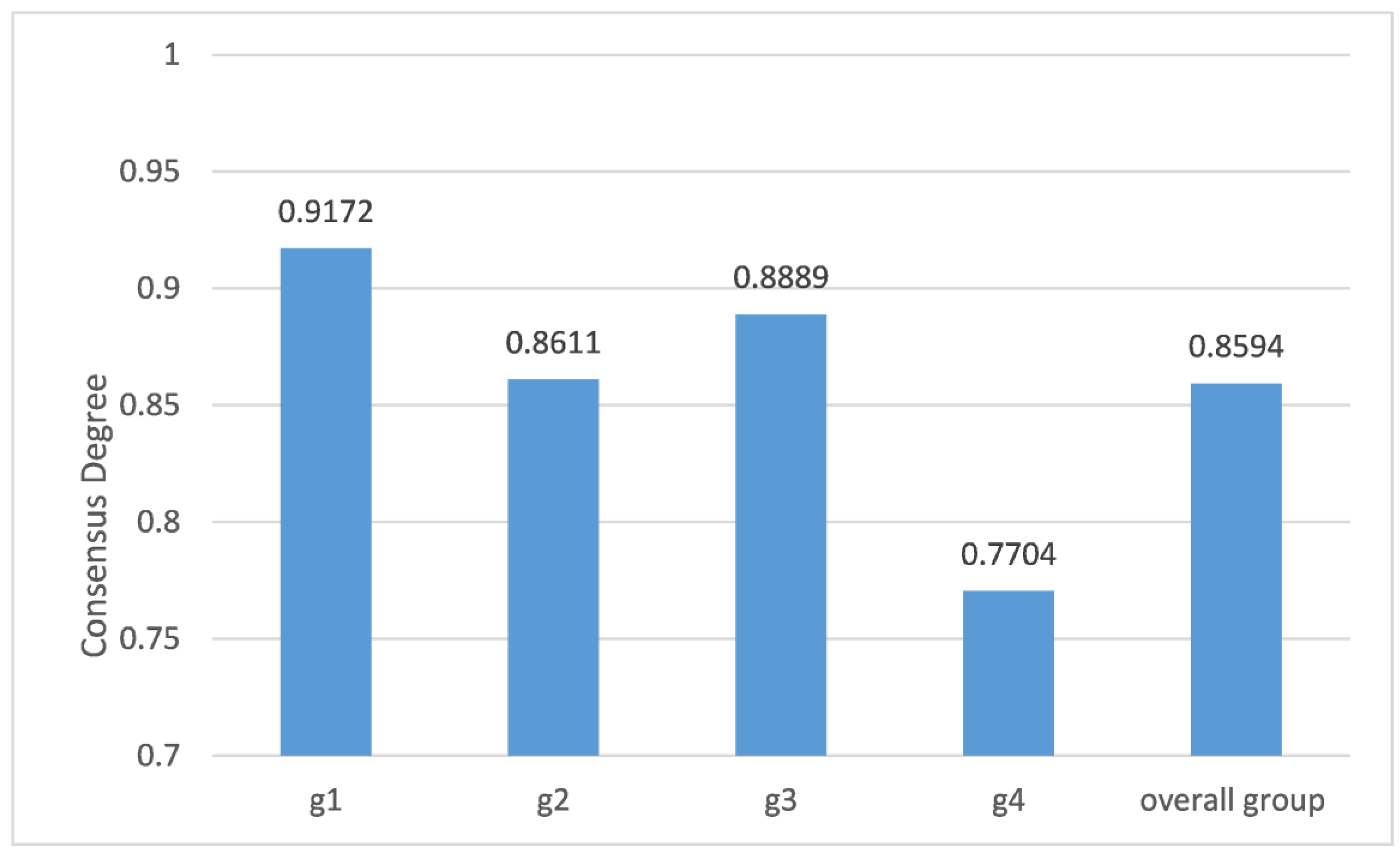
| 0.3333 | 0.9172 | ||
| 0.2667 | 0.8611 | ||
| 0.2667 | 0.8889 | ||
| 0.1333 | 0.7704 |
| Subgroup | ||||
|---|---|---|---|---|
| 0.2941 | 0.2353 | 0.2353 | 0.2353 | |
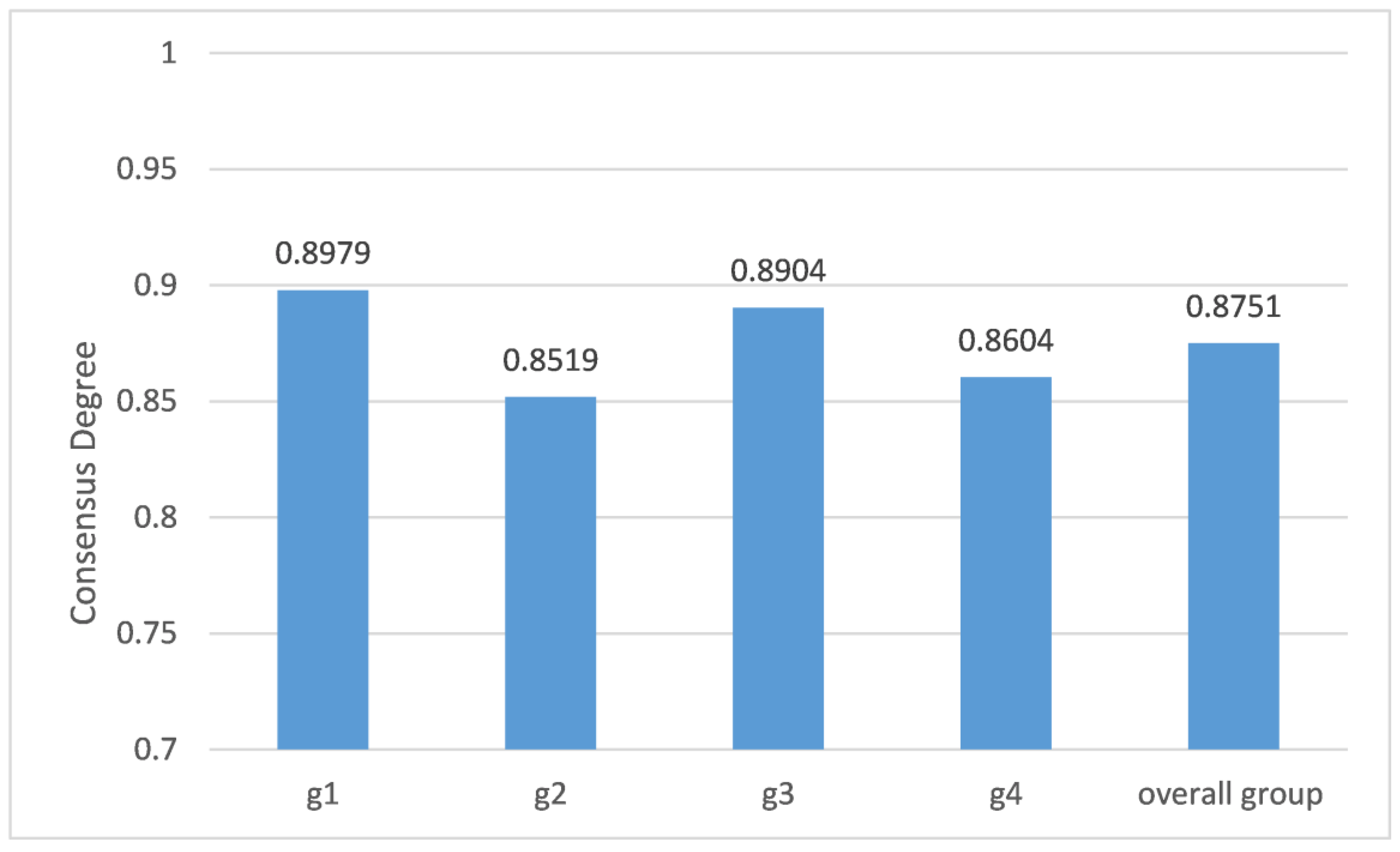
| 0.8979 | 0.8519 | 0.8904 | 0.8604 | |
| 0.8751 | ||||
| Subgroup | ||||
|---|---|---|---|---|
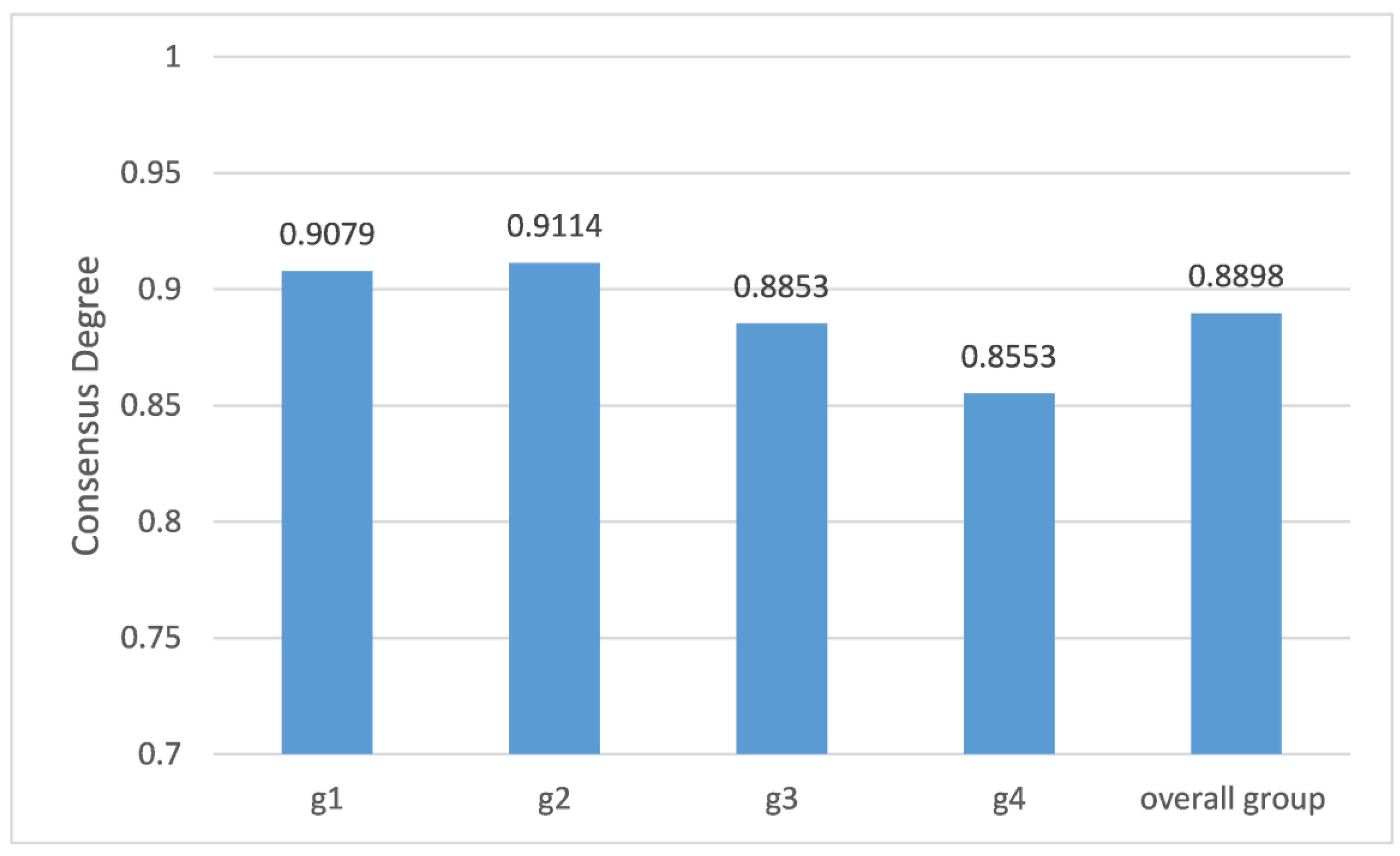
| 0.2941 | 0.2353 | 0.2353 | 0.2353 | |
| 0.9079 | 0.9114 | 0.8853 | 0.8553 | |
| 0.8751 | ||||
| Subgroup | ||||
|---|---|---|---|---|
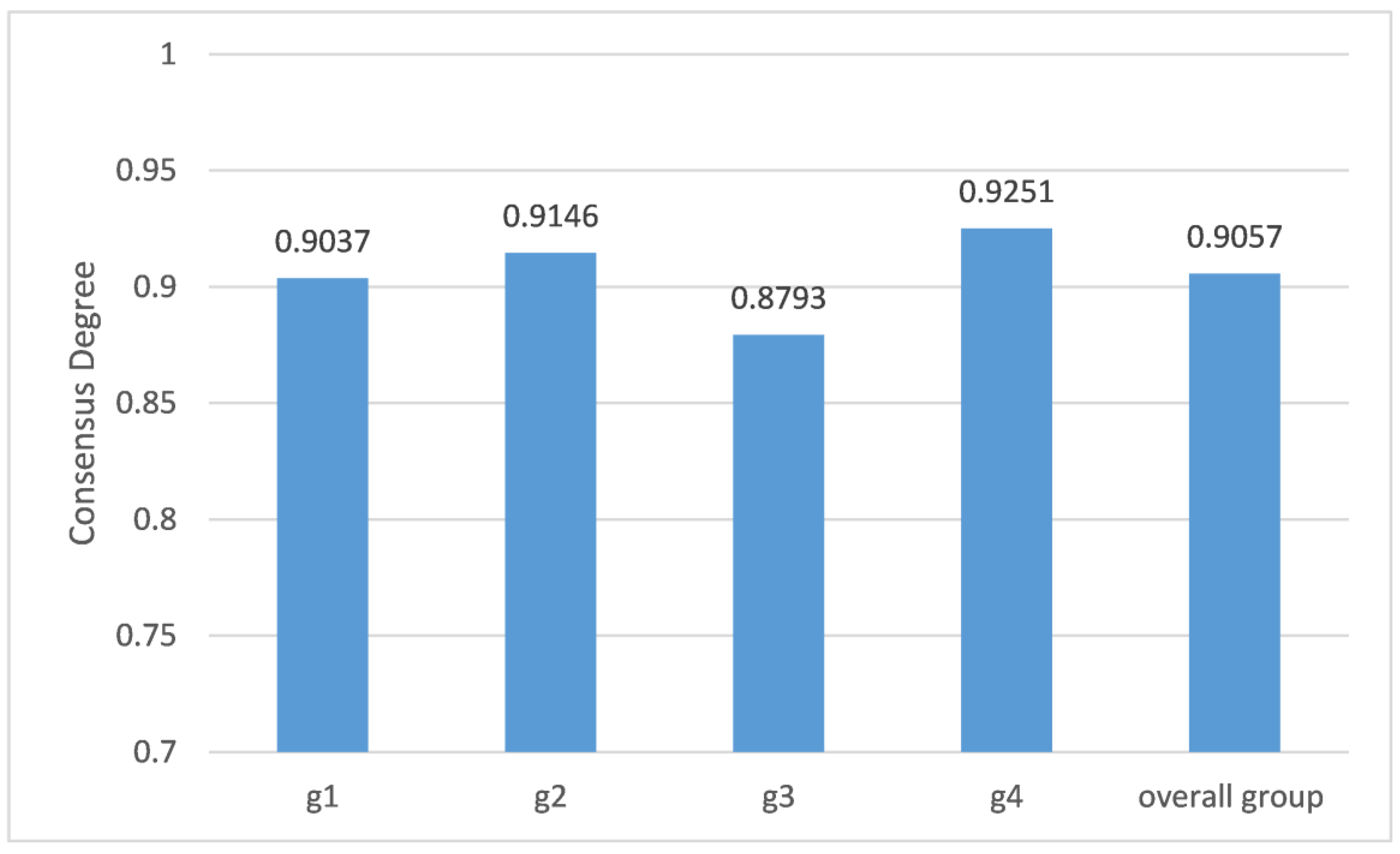
| 0.3012 | 0.2409 | 0.2409 | 0.2169 | |
| 0.9037 | 0.9146 | 0.8793 | 0.9251 | |
| 0.9057 | ||||
| Area | Sichuan | Yunnan | Qinghai | Tibet |
|---|---|---|---|---|
| Subjective score | 0.6312 | 0.5271 | 0.4461 | 0.4871 |
| Objective score | 0.7241 | 0.6563 | 0.5415 | 0.6255 |
| Overall score | 0.6869 | 0.6046 | 0.5033 | 0.5701 |
| Consensus Models | Considering Minority Opinions | Considering Non-Cooperative Behaviors | Considering Linguistic Preference Relation |
|---|---|---|---|
| Li et al. [32] | Not considered | Confidence and social network-based feedback mechanism | Not considered |
| Gai et al. [33] | Not considered | Decentralized feedback mechanism | Not considered |
| Liang et al. [34] | Not considered | Social network-based feedback mechanism | Not considered |
| Zhang et al. [35] | Not considered | Fuzzy rules and optimal allocation-based feedback mechanism | Not considered |
| Liang et al. [36] | Not considered | Two-stage consensus feedback mechanism | Not considered |
| Wu et al. [37]. | Group polarization model considering minority rights and satisfying the majority’s requirements | Not considered | Not considered |
| Ren et al. [38] | Social network-based feedback mechanism | Not considered | Hesitant fuzzy hesitant preference relations |
| Xiao et al. [39] | Extended MULTIMOORA method protecting minority opinions | Not considered | Not considered |
| Zhou et al. [23] | Feedback mechanism | Feedback mechanism | Not considered |
| Xu et al. [27] | Feedback mechanism | Feedback mechanism | Not considered |
| Liu et al. [40] | Not considered | Social network-based feedback mechanism | Linguistic preference relation |
| Zheng et al. [5] | Not considered | Compatibility adjusting process-based feedback mechanism | Hesitant fuzzy linguistic preference relations |
| Zhou et al. [41] | Not considered | Credibility measure-based feedback mechanism | Hesitant fuzzy linguistic preference relations |
| Wan et al. [42] | Not considered | Personalized individual semantics-based feedback mechanism | Probabilistic linguistic preference relations |
| Liao et al. [43] | Not considered | Social network-based feedback mechanism | probabilistic linguistic preference relations |
| Our proposal | Feedback mechanism considering comprehensive adjustment | Feedback mechanism considering comprehensive adjustment | Double-level linguistic preference relation (DLLPR) |
Disclaimer/Publisher’s Note: The statements, opinions and data contained in all publications are solely those of the individual author(s) and contributor(s) and not of MDPI and/or the editor(s). MDPI and/or the editor(s) disclaim responsibility for any injury to people or property resulting from any ideas, methods, instructions or products referred to in the content. |
© 2023 by the authors. Licensee MDPI, Basel, Switzerland. This article is an open access article distributed under the terms and conditions of the Creative Commons Attribution (CC BY) license (https://creativecommons.org/licenses/by/4.0/).
Share and Cite
Yao, J.-C.; Zhou, J.-L.; Xiao, H. A Large-Scale Group Decision-Making Approach to Assess Water Resource Sustainability with Double-Level Linguistic Preference Relation. Water 2023, 15, 2627. https://doi.org/10.3390/w15142627
Yao J-C, Zhou J-L, Xiao H. A Large-Scale Group Decision-Making Approach to Assess Water Resource Sustainability with Double-Level Linguistic Preference Relation. Water. 2023; 15(14):2627. https://doi.org/10.3390/w15142627
Chicago/Turabian StyleYao, Jia-Cheng, Jian-Lan Zhou, and Hai Xiao. 2023. "A Large-Scale Group Decision-Making Approach to Assess Water Resource Sustainability with Double-Level Linguistic Preference Relation" Water 15, no. 14: 2627. https://doi.org/10.3390/w15142627