Multi-Criteria Decision Analyses for the Selection of Hydrological Flood Routing Models

Abstract

In this study, a framework to circumvent the difficulties in selecting a proper flood routing method was established by employing two different multi-criteria decision analysis (MCDA) tools, namely, TOPSIS and PROMETHEE, with definite decisive criteria such as the error metrics, the number of model parameters, and the model background, under three scenarios. For eight distinct flood datasets, the parameters of 10 different Muskingum models were determined using the water cycle optimization algorithm (WCOA) and the performance of each model was ranked by both MCDA tools considering the hydrograph types of flood datasets, labeled as smooth single peak, non-smooth single peak, multi-peak, and irregular. The results indicate that both tools were compatible by giving similar model results in the rankings of almost all scenarios that include different weights in the criteria. The ranking results from both tools also showed that the routing application in single-peak hydrographs was examined better with empirical models that have a high number of parameters; however, complex hydrographs that have more than one peak with irregular limps can be assessed better using the physical-based routing model that has fewer parameters. The proposed approach serves as an extensive analysis in finding a good agreement between measured and routed hydrographs for flood modelers about the estimation capabilities of commonly used Muskingum models considering the importance of correlation, model complexity, and hydrograph characteristics.

1. Introduction

Since flood routing can help to mitigate the possible casualties and infrastructure damage caused by flood events, it is a crucial concern in the fields of hydrology and water resources engineering. Flood routing can be a complex and challenging task, as it involves many variables such as the amount of precipitation, the rate of runoff, the topography of the landscape, and the capacity of the drainage system [1]. In addition to these variables, the selection of proper methods and flow parameters increases the complexity behind the flood routing process. There are a variety of methods that can be used for flood routing, including hydraulic modeling and hydrological modeling with statistical and data-driven models [2]. In these models, the routing flow problem can be solved by considering either distributed or lumped system approaches. Using the distributed routing approach, the continuity and momentum equations, such as the Saint-Venant equation and kinematic or diffusive wave models for unsteady flow, can be used to portray the flow behavior or the movement of the floodwater [3]. Alternatively, lumped routing approaches can be constructed via the continuity equation together with a storage relation expressed as a function of time. The accuracy and the simplicity in use are trade-offs between the aforementioned approaches. While distributed-based approaches are more accurate, lumped-based solutions are simpler to use. However, due to their simplicity, lumped-based routing methods are viable for preliminary routing designs [4].

Being one of the earliest lumped-based routing models, the Muskingum model, proposed by [5], has been used in practice frequently. The linear storage relation is typically formulated as

$$S=K\left[wI+\left(1-w\right)Q\right]$$

(1)

where S is the storage of the control section, I is the inflow and Q is the outflow, K is the storage-time constant, and w is a weighting factor. Over the years, several non-linear Muskingum models have been devised [2,6,7,8,9,10,11]. The extensive literature on the identification of the featured parameters for the models is summarized in

Table 1. Muskingum models with number of parameters and references.

Model No.	Storage Equation *	# of Parameters	Studied by
M1	$S=K[wI+(1-w\left)Q\right]$	2	[5]
M2	$S=K[w{I}^{\alpha }+(1-w)Q^{\alpha }]$	3	[6]
M3	$S=K{[wI+(1-w)Q]}^m$	3	[7]
M4	$S=K{[wI+(1-w)Q]}^{3/5}$	2	[3]
M5	$S=K\left[w\right(1+\gamma )I+(1-w\left)Q\right]$	3	[8]
M6	$S=K[w{I}^{\alpha }+(1-w)Q^{\beta }]$	4	[9]
M7	$S=K{[w{I}^{\alpha }+(1-w)Q^{\alpha }]}^m$	4	[2]
M8	$S=K{[w{I}^{\alpha }+(1-w)Q^{\beta }]}^m$	5	[10]
M9	$S=K{[w(1+\gamma )I+(1-w)Q]}^m$	4	[11]
M10	$S=K{[w(1+\gamma )I^{\alpha }+(1-w)Q^{\beta }]}^m$	6	Proposed

* where $\alpha$ is the flow exponent, m is the general model exponent, $\gamma$ is the lateral flow, and $\beta$ is the flow exponent.

. The classical gradient-based solvers, including non-linear least square (e.g., [12]), Lagrange multiplier (e.g., [13]), the Broyden–Fletcher–Goldfarb–Shanno method (e.g., [14]), and derivative-free optimization methods such as the Nelder–Mead simplex (e.g., [15]) are readily available methods in order to estimate the parameters of non-linear Muskingum models. In addition to these techniques, genetic algorithms (e.g., [16,17]), harmony search (e.g., [18]), particle swarm optimization (e.g., [19]), differential evolution (e.g., [20]), and immune clonal selection (e.g., [21]) are some examples of widely used population-based global optimization algorithms in flood routing. Similarly, the hybridization of population-based algorithms (e.g., [22,23,24,25,26]) is a frequently visited strategy to improve the quality of the parameter estimation procedure.

The aforementioned methods are strong and powerful, there are, however, some issues associated with flood routing procedures as comprehensively discussed in [27]. Some of the storage relations in Table 1 may be grounded on the physical parameters that involve flow characteristics, whereas some include empirical coefficients employed for improving the fit relation between inflow and outflow data. For instance, when $m=3/5$, the M4 form could be obtained from kinematic wave theory for a rectangular channel, as shown by [3]. However, the remaining forms are dimensionally inconsistent, which eventually yields different units of K. Dimensionally consistent models may ensure the attaining of global optima [28]. The routing approach is another important point that may directly affect the estimation performance of the implemented algorithms. Some numerical remedies for the time-marching solution could provide better results [27,28,29,30,31].

As thoroughly summarized, the capability of present models to explain a flood event may be improved by adding either physical or empirical parameters. Comparison assessments for the studied algorithms or the proposed non-linear models by researchers were generally undertaken with the very well-known benchmark dataset provided by [32]. It can be understood from the visited literature that selecting a particular storage model is as significant as the algorithm used in the parameter identification process. However, the decision making about which model works better (at least with an acceptable error level) for any kind of flood data seems to be unanswered yet. Moreover, the results given for the implemented flood data with a specific optimization algorithm may not be adequate to conduct a fair comparison. In addition to the error metrics, which are used as the performance indicators, the model complexity (number of model parameters) and the flood data characteristics (hydrographs with single peak, multi-peak, or irregular, etc.) could allow the researchers to perform an unbiased comparison assessment. This study is intended to fill the mentioned research gap via explaining the performance of different storage models with different number of parameters by employing various flood datasets. This goal was achieved by employing two well-known multi-criteria decision analysis (MCDA) tools. To the best of the authors’ knowledge, such an attempt at evaluating hydrological flood routing models with MCDA tools is one of the first studies in the literature.

2. Data and Methods

In this section, we first explain the routing approach followed by the flood routing optimization and flood datasets. The parameters of the Muskingum models implemented in this study are obtained by using the water cycle optimization algorithm (WCOA) whose details are given in the following subsections. Then, the datasets collected from previous studies are introduced. Finally, multi-criteria decision analysis tools are discussed in detail. Figure 1 summarizes the entire work flow behind this study.

2.1. Routing Approach

The mass balance equation is

$$\frac{dS\left(t\right)}{dt}=\left(1+\gamma \right)I\left(t\right)-Q\left(t\right)$$

(2)

where S is the storage of the control section, I is the inflow and Q is the outflow, and $\gamma$ is the lateral flow coefficient. The general non-linear Muskingum model can be written as

$$S=K{\left[w\left(1+\gamma \right)I^{\alpha }+\left(1-w\right)Q^{\beta }\right]}^m$$

(3)

in which K is the storage-time constant, w is the weighting factor, $\alpha$ is the inflow exponent, $\beta$ is the outflow exponent, and m is the general model exponent. Equation (3) can be rearranged for estimating the outflow as

$$Q={\left[\frac{1}{\left(1-w\right)}{\left(\frac{S}{K}\right)}^{\frac{1}{m}}-\frac{w}{\left(1-w\right)}\left(1+\gamma \right)I^{\alpha }\right]}^{\frac{1}{\beta }}$$

(4)

For any particular time level of $i+1$, Equation (4) can be expressed as

$$Q_{i+1}={\left[\frac{1}{\left(1-w\right)}{\left(\frac{S_{i+1}}{K}\right)}^{\frac{1}{m}}-\frac{w}{\left(1-w\right)}\left(1+\gamma \right)I_{i+1}^{\alpha }\right]}^{\frac{1}{\beta }}$$

(5)

for $i=1,2,\dots ,N-1$, where N is the total number of observed data. As discussed in [27], the use of weighted $I_i$ and $I_{i+1}$ could give better performance than using $I_{i+1}$ only. Therefore, the $I_{i+1}$ term in Equation (5) is replaced with

$$I_{i+1}=\eta I_i+\left(1-\eta \right)I_{i+1}$$

(6)

in which $\eta$ is the weight coefficient of the explicit–implicit scheme. Equation (5) is then

$$Q_{i+1}={\left[\frac{1}{\left(1-w\right)}{\left(\frac{S_{i+1}}{K}\right)}^{\frac{1}{m}}-\frac{w}{\left(1-w\right)}\left(1+\gamma \right){\left(\eta I_i+\left(1-\eta \right)I_{i+1}\right)}^{\alpha }\right]}^{\frac{1}{\beta }}$$

(7)

When the finite difference formulation is applied to Equation (2), it becomes

$$\frac{S_{i+1}-S_i}{∆t}=\left(1+\gamma \right)I_i-{\left[\frac{1}{\left(1-w\right)}{\left(\frac{S_i}{K}\right)}^{\frac{1}{m}}-\frac{w}{\left(1-w\right)}\left(1+\gamma \right)I_i^{\alpha }\right]}^{\frac{1}{\beta }}$$

(8)

where $∆t$ denotes the time interval. If the right-hand side terms of Equation (8) are denoted by $F_i$, it will be then

$$S_{i+1}=S_i+F_i∆t$$

(9)

The flood routing process starts with the assumed initial conditions ($I_0=I_1$ and $Q_0=Q_1$). Thus, the initial storage will be

$$S_1=K{\left[w\left(1+\gamma \right)I_0^{\alpha }+\left(1-w\right)Q_0^{\beta }\right]}^m$$

(10)

As a summary, the following computation steps complete the routing process:

Step 1:

Compute the initial storage ($i=1$) using Equation (10).

Step 2:

Compute $S_{i+1}$ using Equation (9).

Step 3:

Estimate $Q_{i+1}$ using Equation (7).

Step 4:

Go to step 2. Repeat the remaining computations for $i=2,3,\dots ,N-1$ data points.

2.2. Flood Routing Optimization

As given in Table 1, each implemented Muskingum model has a different number of model parameters, ranging from 2 to 6, and their values can be found by minimizing the cost function which is the discrepancy between the observed outflow data and estimated outflow values. When minimizing the cost function, negative storage and outflow values may appear during the space search for the optimum model parameters. Since negative values for the storage and outflow are physically impossible, such situations are regarded as the constraints of the optimization problem of interest. Therefore, the cost function with the penalized constraints can be written as

$$C=\sum _{i=1}^N{\left[Q_{obs,i}-Q_i\left(K,w,\gamma ,\alpha ,\beta ,m,\eta \right)\right]}^2+{\varphi }_i+{\psi }_i$$

(11)

where Q is the estimated outflow computed by Equation (7) and the penalty functions $\varphi$ and $\psi$ are

$${\varphi }_i=\left\{\begin{array}{c}{\lambda }_1\left|S_{i+1}\right|\hspace{1em}if\hspace{1em}{S}_{i+1}<0\\ 0\hspace{1em}otherwise\end{array}\right.$$

(12)

and

$${\psi }_i=\left\{\begin{array}{c}{\lambda }_2\left|Q_{i+1}\right|\hspace{1em}if\hspace{1em}{Q}_{i+1}<0\\ 0\hspace{1em}otherwise\end{array}\right.$$

(13)

where ${\lambda }_1$ and ${\lambda }_2$ are the penalty coefficients. In this study, ${\lambda }_1$ and ${\lambda }_2$ are assumed to be 0.5. Note that when the storage and the computed outflow values are negative, their penalty values are assumed to be equal in order to continue the flood routing process as outlined in the previous section.

In order to find the optimum model parameters for the cost function given by Equation (11), the space search could be achieved by the water cycle optimization algorithm (WCOA). This was first proposed by [33] for attaining global optima by mimicking the water cycle processes such as forming rivers, streaming, running to the sea, rainfall, and evaporation. The WCOA is constructed on the analogy that streams reach to rivers, rivers are running to the sea. In other words, the candidate solutions will be eliminated under some certain rules of the algorithm, and the best possible solution set, known as sea, will finally satisfy the global optima during the iterations. Suppose $C=Cost\left(x\right)$ is the cost function to be minimized with its d-dimensional variable set $x=\left\{x_1,x_2,\dots ,x_d\right\}$. For a user-defined population size of $N_{pop}$, the WCOA starts by generating random candidate solution sets ($i=1,2,\dots ,N_{pop}$) for the optimized parameter set ($j=1,2,\dots ,d$) as

$$x_{i,j}^{\left(0\right)}=x_j^{L_B}+{\Omega }_{i,j}\times \left(x_j^{U_B}-x_j^{L_B}\right)$$

(14)

where $x_j^{L_b}$ and $x_j^{U_b}$ are the lower and upper bounds of the optimized parameters, respectively, ${\Omega }_{i,j}$ is a uniform random number generator (${\Omega }_{i,j}\in \left[0,1\right]$), and superscript $\left(0\right)$ denotes the initial solution at the beginning of the iterations. Once the initial values of the parameters are generated via Equation (14), the corresponding cost function values are evaluated by Equation (11) and sorted with respect to their minimum to maximum values. Then, the sorted positions are grouped as

$$X=\left[\begin{array}{c}Sea\\ Rive{r}_1\\ Rive{r}_2\\ ·\\ Rive{r}_{N_r}\\ Strea{m}_{N_{sr+1}}\\ Strea{m}_{N_{sr+2}}\\ ·\\ ·\\ Strea{m}_{N_{stream}}\end{array}\right]=\left[\begin{array}{ccccc}{x}_1^1& x_2^1& ·& ·& x_d^1\\ x_1^2& x_2^2& ·& ·& x_d^2\\ ·& ·& ·& ·& ·\\ ·& ·& ·& ·& ·\\ x_1^{N_{pop}}& x_2^{N_{pop}}& .& .& x_d^{N_{pop}}\end{array}\right]$$

(15)

with

$$\begin{array}{c}{N}_{sr}=N_r+1\hfill \\ N_{stream}=N_{pop}-N_{sr}\hfill \end{array}$$

(16)

where $N_r$ is the number of rivers, $N_{sr}$ is the total number of rivers and the sea, and finally $N_{stream}$ is the number of streams. Thus,

$$\begin{array}{c}{X}_{sea}=X(1,:)\hfill \\ X_{river}=X(2:N_r,:)\hfill \\ X_{stream}=X(N_{sr}+1:N_{stream},:)\hfill \end{array}$$

(17)

By this notation, $X\left(a:b,:\right)$ shows the entries of matrix X from the ath row to the bth row with all columns. As a next step, some of the streams reach the rivers, rivers are running to the sea. By means of this analogy, some solution sets will be stored through iterations and new solution sets will be created as follows

$$N{S}_i=round\left\{\left|\frac{C_i}{{\sum }_{i=1}^{N_{sr}}{C}_i}\right|\times N_{stream}\right\}$$

(18)

where $N{S}_i$ is the certain number of streams reaching the rivers or sea and $C_i=Cos{t}_i-Cos{t}_{N_{sr+1}}$ for $i=1,2,\dots ,N_{sr}$. Note that Equation (18) creates an array with a length of $N_{sr}$ and ${\sum }_{i=1}^{N_{sr}}NS\left(i\right)=N_{stream}$. The positions of the streams, rivers, and sea for each individual member of a d-dimensional variable set will be updated for the next iteration. The streams may reach to the sea directly. Therefore, the stream positions should be updated according to the position of sea as

$$X_{stream}^{\left(t+1\right)}\left(i,:\right)=X_{stream}^{\left(t\right)}\left(i,:\right)+\Omega \Psi \left(X_{sea}^{\left(t\right)}-X_{stream}^{\left(t\right)}\left(i,:\right)\right)$$

(19)

for $i=1,2,\dots ,NS\left(1\right)$, where $\Omega$ denotes a uniform random generator vector with a length of d and $\Psi$ is a controlling parameter varying $\Psi \in \left[1,2\right]$ [34]. Similarly, the streams may run to the rivers. The update mechanism for this case is

$$X_{stream}^{\left(t+1\right)}\left(j,:\right)=X_{stream}^{\left(t\right)}\left(j,:\right)-\Omega \Psi \left(X_{river}^{\left(t\right)}\left(k,:\right)-X_{stream}^{\left(t\right)}\left(j,:\right)\right)$$

(20)

for $j=NS\left(1\right)+1,NS\left(1\right)+2,\dots ,N_{stream}$ and $k=1,2,\dots ,N_{sr}-1$. Finally, the rivers may flow to the sea. The river positions will then be updated as

$$X_{river}^{\left(t+1\right)}\left(i,:\right)=X_{river}^{\left(t\right)}\left(i,:\right)-\Omega \Psi \left(X_{sea}^{\left(t\right)}-X_{river}^{\left(t\right)}\left(i,:\right)\right)$$

(21)

for $i=1,2,\dots ,N_{sr}-1$. Then, the evaporation phase, which means that some of the streams or rivers will be discarded from the candidate solution set in order to prevent stacking the local optima, triggers the precipitation phase, which forms new streams or rivers, with certain rules. For precipitation to a river, the new stream will be formed as

$$\begin{array}{c}if∥X_{sea}^{\left(t\right)}-X_{river}^{\left(t\right)}\left(i,:\right)∥<d_{max}\left|\right|rand<0.1\hfill \\ X_{stream}^{new,\left(t\right)}\left(k,j\right)=x_j^{LB}+rand\times \left(x_j^{UB}-x_j^{LB}\right)\hfill \end{array}$$

(22)

for $i=1,2,\dots ,N_{sr}-1$, $j=1,2,\dots ,d$ and $k=NS\left(1\right)+1,NS\left(1\right)+2,\dots ,N_{stream}$, where $rand$ is a uniform random number, $\parallel .\parallel$ is the Euclidean norm, and $d_{max}$ is the user-specified small control number which provides searching intensity around the comparison norm. Similarly, when precipitation comes to the streams, a new stream will be generated as

$$\begin{array}{c}if∥X_{sea}^{\left(t\right)}-X_{stream}^{\left(t\right)}\left(i,:\right)∥<d_{max}\left|\right|rand<0.1\hfill \\ X_{stream}^{new,\left(t\right)}\left(i,j\right)=x_j^{LB}+rand\times \left(x_j^{UB}-x_j^{LB}\right)\hfill \end{array}$$

(23)

for $i=1,2,\dots ,NS\left(1\right)$. Through the iterations, $d_{max}$ can be adjusted as

$$d_{max}^{\left(t+1\right)}=d_{max}^{\left(t\right)}-\frac{d_{max}^{\left(t\right)}}{i{t}_{max}}$$

(24)

where $i{t}_{max}$ shows the maximum iteration number [35]. In this study, the WCOA is utilized with $N_{pop}=200$ and $i{t}_{max}=1000$.

2.3. Flood Datasets

The outlined WCOA is applied to several flood datasets for identifying the model parameters of each Muskingum model. Each dataset is categorized in terms of its characteristic shape such as smooth single peak (SSP), non-smooth single peak (NSP), multi-peak (MP), and irregular as summarized in Table 2 and shown in Figure 2.

As an SSP-type dataset, Wilson’s 1974 flood [32] is labeled as DS1 in this particular study, which is a classical benchmark dataset previously used in many studies. Brutsaert’s data (DS2) as SSP was tested by [27]. River Wye flood data (DS3 and DS7) have again been examined in several studies (e.g., [29,30,31]) and were collected from the River Wye in England. DS4, provided by [36], is associated with the flood event that occurred in the Karun river in the southwest part of Iran. Viessman and Lewis’s data is a classic example of a two-peak hydrograph, which was used to demonstrate the performance of the proposed algorithms and Muskingum models (e.g., [2,31]). Sütçüler flood (DS6), with two peaks, was gathered from Turkey [11,26]. Finally, DS8, which seems to not have a classical hydrograph shape with an apparent peak, was taken from the south canal of Chenggou and Lingqing river in China. It was also studied by [27,37].

Table 2. Flood datasets, their labels, sources, and hydrograph categories in the study.

Flood Name	Label	Source	Hydrograph Category
Wilson’s 1974 flood	DS1	[32]	Smooth Single Peak
Brutsaert’s data	DS2	[38]	Smooth Single Peak
River Wye 1960 flood	DS3	in [27]	Non-smooth Single Peak
Karun river flood	DS4	[36]	Non-smooth Single Peak
Viessman and Lewis’s data	DS5	[39]	Multi-Peak
Sütçüler flood	DS6	[11]	Multi-Peak
River Wye 1982 flood	DS7	in [11]	Irregular
Chenggou and Lingqing river	DS8	[37]	Irregular

Table 2. Flood datasets, their labels, sources, and hydrograph categories in the study.

Flood Name	Label	Source	Hydrograph Category
Wilson’s 1974 flood	DS1	[32]	Smooth Single Peak
Brutsaert’s data	DS2	[38]	Smooth Single Peak
River Wye 1960 flood	DS3	in [27]	Non-smooth Single Peak
Karun river flood	DS4	[36]	Non-smooth Single Peak
Viessman and Lewis’s data	DS5	[39]	Multi-Peak
Sütçüler flood	DS6	[11]	Multi-Peak
River Wye 1982 flood	DS7	in [11]	Irregular
Chenggou and Lingqing river	DS8	[37]	Irregular

2.4. Comparison of Muskingum Models

The Muskingum models in Table 1 are ranked with certain criteria such as the error metrics with normalized root mean squared error (N-RMSE) and the adjusted coefficient of determination ($Ad-R^2$). The model complexity, which is characterized by the number of optimized parameters for each model (NP), and the model background (MB) that shows whether the model parameters are physical or empirical. The N-RMSE and $Ad-R^2$, which are the performance indicators of the WCOA-assisted parameter estimation for each dataset, can be, respectively, calculated by

$$N-RMSE=\frac{\sqrt{{\sum }_{i=1}^N{\left(y_i-s_i\right)}^2}}{\left(y_{max}-y_{min}\right)}$$

(25)

and

$$Ad-R^2=1-\frac{\left(1-R^2\right)\left(N-1\right)}{N-NP-1}$$

(26)

with

$$R^2=1-\frac{{\sum }_{i=1}^N{\left(y_i-s_i\right)}^2}{{\sum }_{i=1}^N{\left(y_i-\overline{y}\right)}^2}$$

(27)

where N is the sample size, $NP$ is the number of optimized parameters used in the model, $y_i$ is the observed ith data value, and $s_i$ is the calculated ith data value. $y_{max}$, $y_{min}$, and $\overline{y}$ are the maximum, minimum, and mean of the observed data values, respectively. As expected, the model with the smallest N-RMSE will be superior. Furthermore, higher $Ad-R^2$ values point out the powerful estimation performance. A lower NP is preferred. Finally, the models with physical parameters could be better to explain a flood event by providing the link between theory and practice.

To conduct a fair and unbiased comparison assessment, multi-criteria decision analysis (MCDA) tools including the technique for order of preference by similarity to ideal solution (TOPSIS) [40,41,42] and the preference ranking organization method for enrichment evaluation (PROMETHEE) [43] are employed to rank the alternatives (they are Muskingum models in Table 1) under definite criteria (N-RMSE, $Ad-R^2$, NP, and MB).

Suppose $A=\left\{a_1,a_2,\dots ,a_p\right\}$ is a p-dimensional alternative set, $C=\left\{c_1,c_2,\dots ,c_r\right\}$ is an r-dimensional criterion set, and Z is the decision matrix as follows

$$Z=\left[\begin{array}{ccccc}{c}_1\left(a_1\right)& c_2\left(a_1\right)& ·& ·& c_r\left(a_1\right)\\ c_1\left(a_2\right)& c_2\left(a_2\right)& ·& ·& c_r\left(a_2\right)\\ ·& ·& ·& ·& ·\\ ·& ·& ·& ·& ·\\ c_1\left(a_p\right)& c_2\left(a_p\right)& ·& ·& c_r\left(a_p\right)\end{array}\right]={\left[\begin{array}{ccccc}{z}_{11}& z_{12}& ·& ·& z_{1r}\\ z_{21}& z_{22}& ·& ·& z_{2r}\\ ·& ·& ·& ·& ·\\ ·& ·& ·& ·& ·\\ z_{p1}& z_{p2}& ·& ·& z_{pr}\end{array}\right]}_{p\times r}$$

(28)

Once the decision matrix is constructed as shown in Equation (28), the TOPSIS method consists of the following steps:

Step 1:

The entries of decision matrix Z are normalized as

$$h_{ij}=\frac{z_{ij}}{\sqrt{{\sum }_{i=1}^p{z}_{ij}^2}},\hspace{1em}i=1,2,\dots ,p,\hspace{1em}j=1,2,\dots ,r$$

(29)

Step 2:

Each criterion has a definite weight such that ${\sum }_{i=1}^r{w}_i=1$. The weighted normalized matrix is then computed as

$$v_{ij}=w_j\times h_{ij},\hspace{1em}i=1,2,\dots ,p,\hspace{1em}j=1,2,\dots ,r$$

(30)

Step 3:

As stated earlier, some criteria can be maximized (a higher value is preferred) or minimized (a lower value is preferred). The ideal best $V^{+}$ and the ideal worst $V^{-}$ solutions are, respectively, determined as

$$V_j^{+}=\left\{\begin{array}{c}max\left(v_{ij}\right), if c_j \mathrm{is} \mathrm{maximized}\\ min\left(v_{ij}\right), if c_j \mathrm{is} \mathrm{minimized}\end{array}\right. i=1,2,\dots ,p j=1,2,\dots ,r$$

(31)

$$V_j^{-}=\left\{\begin{array}{c}min\left(v_{ij}\right), if c_j \mathrm{is} \mathrm{maximized}\\ max\left(v_{ij}\right), if c_j \mathrm{is} \mathrm{minimized}\end{array}\right. i=1,2,\dots ,p j=1,2,\dots ,r$$

(32)

Step 4:

The Euclidean distance for the ideal best and the ideal worst solutions will be

$${\zeta }_i^{+}=\sqrt{\sum _{i=1}^r{\left(v_{ij}-V_j^{+}\right)}^2} i=1,2,\dots ,p j=1,2,\dots ,r$$

(33)

and

$${\zeta }_i^{-}=\sqrt{\sum _{i=1}^r{\left(v_{ij}-V_j^{-}\right)}^2} i=1,2,\dots ,p j=1,2,\dots ,r$$

(34)

Step 5:

The closeness to the ideal solution for each alternative is then computed by

$${\chi }_i=\frac{{\zeta }_i^{-}}{{\zeta }_i^{-}+{\zeta }_i^{+}} i=1,2,\dots ,p$$

(35)

Step 6:

Finally, ${\chi }_i$ values are sorted. A larger $\chi$ value implies a better alternative.

For PROMETHEE, the computational process is as follows:

Step 1:

Step 1: The decision matrix Z in Equation (28) is normalized first according to the criteria whether some of them are maximized or minimized as

$$z_{ij}=\left\{\begin{array}{c}\frac{c_j\left(a_i\right)-min\left(c_j\right)}{max\left(c_j\right)-min\left(c_j\right)}, if c_j \mathrm{is} \mathrm{maximized}\\ \frac{max\left(c_j\right)-c_i\left(a_i\right)}{max\left(c_j\right)-min\left(c_j\right)}, if c_j \mathrm{is} \mathrm{minimized}\end{array}\right. i=1,2,\dots ,p j=1,2,\dots ,r$$

(36)

Step 2:

The pairwise distance is

$$d_k(a_i,a_j)=c_k\left(a_i\right)-c_k\left(a_j\right) i\ne j, i,j=1,2,\dots ,p k=1,2,\dots ,r$$

(37)

where $d_k$ is the distance between the normalized ith alternative and jth alternative for the kth criterion. Therefore, a total of $r\times (p-1)$ pairwise distances is computed.

Step 3:

The preference degree is then determined by a preference function as

$$\pi (a_i,a_j)=\sum _{k=1}^r{P}_k\left(d_k\left(a_i,a_j\right)\right)w_k$$

(38)

where P is the preference function. In this study, the binary preference function is used as

$$P\left(d_k\right)=\left\{\begin{array}{c}0, if d_k\le 0\\ 1, if d_k>0\end{array}\right.$$

(39)

Thus, $\pi$ values can be expressed by a $p\times p$ matrix whose diagonal entries are empty as

$$\Gamma ={\left[\begin{array}{cccccc}-& \pi (a_1,a_2)& \pi (a_1,a_3)& ·& ·& \pi (a_1,a_p)\\ \pi (a_2,a_1)& -& \pi (a_2,a_3)& ·& ·& \pi (a_2,a_p)\\ ·& ·& ·& ·& ·& ·\\ \pi (a_p,a_1)& \pi (a_p,a_2)& ·& ·& \pi (a_{p-1},a_p)& -\end{array}\right]}_{p\times p}$$

(40)

Step 4:

The ideal best (positive flow) and the ideal worst (negative flow) solutions are

$${\xi }_i^{+}\left(a_i\right)=\frac{1}{p-1}\sum _{i=1}^p\pi \left(a_i,x\right)$$

(41)

and

$${\xi }_i^{-}\left(a_i\right)=\frac{1}{p-1}\sum _{i=1}^p\pi \left(x,a_i\right)$$

(42)

In other words, ${\xi }_i^{+}$ is the mean of the ith row of matrix $\Gamma$, whereas ${\xi }_i^{-}$ is the mean of the ith column of matrix $\Gamma$.

Step 5:

The ideal solution (net flow) is

$${\xi }_i\left(a_i\right)={\xi }_i^{+}\left(a_i\right)-{\xi }_i^{-}\left(a_i\right)$$

(43)

Step 6:

The PROMETHEE provides the complete ranking by ordering alternatives according to the decreasing values of the ideal solution $\xi$.

As a summary, the comparison assessment of Muskingum models is conducted via the following scheme:

1.

The parameters of each model in Table 1 are estimated by the WCOA for each dataset given in Table 2.

2.

The computed outflow values obtained from (1) are substituted into Equations (25) and (26) in order to obtain the N-RMSE and $Ad-R^2$ values of each model for the particular dataset.

3.

For each dataset, the estimation score of each model is noted and sorted. Since there is a total of 10 models, the model with the smallest N-RMSE is given a rank of 1 while the highest one is given a rank of 10. A smaller rank indicates a better performance.

4.

Based on the N-RMSE values, the ranks for each dataset are found and then averaged.

5.

Similarly, the $Ad-R^2$ values of each model for each dataset are sorted. The model with the highest $Ad-R^2$ value is given a rank of 1 while the smallest one is given a rank of 10. A higher rank score shows a better performance.

6.

With $Ad-R^2$ values, the rank scores are averaged.

7.

The decision matrix is formed by NP and MB together with the rank scores of N-RMSE and $Ad-R^2$. A binary code (1 for the models with physical parameters, 0 for the models with empirical parameters) is used to classify the MB.

8.

The obtained decision matrix acquired from the previous steps is then studied by TOPSIS and PROMETHEE to elucidate the most efficient Muskingum model.

3. Results and Discussion

3.1. Estimation Performance of Models

Following the WCOA-based parameter estimation approach detailed in the previous section, the model parameters of the Muskingum models listed in Table 1 were obtained using the datasets of eight distinct flood events. For each flood event, the parameters and prediction performance of the models used are presented in

Table A1. Results for the parameter estimation for each model and each dataset ($\alpha$ is the flow exponent, m is the general model exponent, $\gamma$ is the lateral flow, $\beta$ is the flow exponent, and $\eta$ is the coefficient of the explicit/implicit scheme).

Dataset	Model	K	w	$\mathit{\gamma }$	$\mathit{\alpha }$	$\mathit{\beta }$	m	$\mathit{\eta }$	SSE	$\mathit{Ad}-{\mathit{R}}^2$	N-RMSE	MAE
DS 1	M1	29.8106	0.2388					1	415.55	0.9624	0.0659	3.77
	M2	2.7637	0.2287		1.5012			1	245.58	0.9766	0.0506	2.76
	M3	0.5175	0.2869				1.8681	1	36.77	0.9965	0.0196	1.07
	M4	235.8340	0.1661				0.6000	1	752.00	0.9320	0.0886	4.96
	M5	29.7496	0.2477	−0.0091				1	411.69	0.9607	0.0655	3.74
	M6	1.6247	0.0003		3.0418	1.5676		1	184.32	0.9814	0.0439	2.45
	M7	0.8338	0.2956		0.4331		4.0790	1	7.67	0.9992	0.0089	0.47
	M8	0.8646	0.0395		0.7438	0.3679	4.3500	0.9307	4.96	0.9995	0.0072	0.29
	M9	0.5342	0.3005	−0.0216			1.8642	1.0	9.82	0.9990	0.0101	0.57
	M10	0.6663	0.0246	−0.0077	0.9850	0.4953	3.3866	0.8657	4.09	0.9995	0.0065	0.31
DS 2	M1	2.0839	0.1102					1	15,895.60	0.9987	0.0109	16.73
	M2	1.0809	0.1332		1.0839			0.9602	11,846.22	0.9990	0.0094	14.73
	M3	0.8189	0.0388				1.1107	0	12,144.80	0.9990	0.0095	14.95
	M4	51.9261	0.0000				0.6000	0.5320	155,580.39	0.9874	0.0341	53.38
	M5	2.0077	0.0251	0.0129				1	11,913.60	0.9990	0.0094	15.04
	M6	586.1200	0.9992		0.2314	1.1572		0.9554	8631.99	0.9992	0.0080	12.78
	M7	1.5962	0.1616		1.7865		0.5823	1.0000	8244.86	0.9993	0.0078	12.31
	M8	0.9137	0.0001		5.0000	4.0957	0.2687	0.5103	7711.48	0.9993	0.0076	11.77
	M9	1.1235	0.0560	0.0117			1.0746	1.0000	9043.47	0.9992	0.0082	12.48
	M10	13.6508	0.9675	0.0041	0.8243	1.4851	0.7180	0.8723	8510.25	0.9992	0.0080	12.45
DS 3	M1	26.6573	0.4274					1	88,387.01	0.9431	0.0565	36.16
	M2	1.6370	0.4024		1.4050			1	44,478.76	0.9704	0.0401	25.01
	M3	0.4624	0.4091				1.5856	1	35,194.51	0.9766	0.0356	22.65
	M4	491.3309	0.3475				0.6000	1	200,258.51	0.8711	0.0850	58.54
	M5	26.4413	0.3992	0.0465				1	82,057.20	0.9454	0.0544	35.47
	M6	0.6773	0.0022		2.2497	1.4641		1	37,352.54	0.9743	0.0367	20.56
	M7	0.4502	0.4074		1.2022		1.3229	1	29,474.96	0.9797	0.0326	20.19
	M8	0.9540	0.7331		1.0038	1.1888	1.3742	1	29,132.20	0.9792	0.0324	20.41
	M9	0.3691	0.3830	0.0547			1.6141	1	25,915.27	0.9822	0.0306	17.09
	M10	0.7500	0.0452	0.1323	0.5429	0.2676	5.0000	1	20,048.64	0.9852	0.0269	14.51
DS 4	M1	12.5606	0.2424					1	89,417.76	0.9735	0.0544	31.20
	M2	1000	0.1846		0.4563			1	65,726.23	0.9801	0.0466	27.22
	M3	1000	0.1749				0.4570	1	64,593.54	0.9804	0.0462	27.07
	M4	297.3967	0.1989				0.6000	1	68,814.88	0.9796	0.0477	28.12
	M5	12.3521	0.3608	−0.0314				1	63,325.14	0.9808	0.0458	27.55
	M6	1000	0.1101		0.5159	0.4462		1	65,666.31	0.9796	0.0466	27.19
	M7	1000	0.1146		2.8707		0.1600	1	62,607.58	0.9806	0.0455	27.00
	M8	1000	0.0000		5.0000	3.4967	0.1301	1	60,243.11	0.9808	0.0446	26.12
	M9	980.2646	0.2431	−0.0198			0.4564	1	54,947.64	0.9829	0.0426	25.64
	M10	1000	0.0000	−0.0249	5.0000	2.8688	0.1551	1	47,663.45	0.9845	0.0397	22.80
DS 5	M1	3.8158	0.4489					1	14.53	1.0000	0.0006	0.62
	M2	3.8376	0.4490		0.9993			1	13.98	1.0000	0.0006	0.60
	M3	3.8003	0.4489				1.0005	1	14.33	1.0000	0.0006	0.62
	M4	83.3925	0.3243				0.6000	1	118,587.65	0.9725	0.0513	57.10
	M5	3.8174	0.4497	−0.0007				1	7.57	1.0000	0.0004	0.21
	M6	3.7546	0.4300		1.0074	0.9978		1	10.56	1.0000	0.0005	0.42
	M7	3.7960	0.4490		0.9952		1.0055	1	8.96	1.0000	0.0004	0.36
	M8	3.7918	0.4476		0.9960	0.9953	1.0052	1	8.95	1.0000	0.0004	0.36
	M9	3.7977	0.4496	−0.0007			1.0007	1	7.24	1.0000	0.0004	0.22
	M10	3.7721	0.4411	−0.0007	1.0053	1.0010	0.9986	1	6.98	1.0000	0.0004	0.22
DS 6	M1	1.0478	0.0000					0	561.30	0.9903	0.0217	3.12
	M2	1000	0.6980		5.0000			0.9836	327.35	0.9941	0.0166	1.86
	M3	0.9867	0.0000				1.0106	0.9995	560.62	0.9899	0.0217	3.14
	M4	11.4763	0.0000				0.6000	0.9895	1979.65	0.9657	0.0408	6.19
	M5	0.5197	0.9999	−1.0001				0.9802	283.39	0.9949	0.0154	1.68
	M6	1000	0.7460		5.0000	5.0535		0.9877	322.01	0.9940	0.0165	1.92
	M7	0.0100	0.6980		5.0000		4.7868	0.9836	327.35	0.9939	0.0166	1.86
	M8	1.2950	0.0091		0.6912	0.1798	5.0000	1	319.37	0.9938	0.0164	1.94
	M9	126.2182	−1.0000	0.8970			5.0000	0.9945	292.35	0.9945	0.0157	1.82
	M10	1000	0.3908	−2.6209	1.6807	1.7052	1.9928	0.9996	280.56	0.9943	0.0154	1.81
DS 7	M1	131.5774	0.9917					0.9561	36,896.67	−0.3563	0.3752	26.36
	M2	307.8855	0.7268		0.4827			0.2951	5272.04	0.7993	0.1418	10.04
	M3	1000	0.9622				0.2656	0.4545	24,252.22	0.0766	0.3042	16.28
	M4	325.5926	0.9808				0.6000	0.8240	25,624.60	0.0580	0.3127	17.65
	M5	5.1523	0.2293	2.5276				1	54.86	0.9979	0.0145	0.95
	M6	341.8120	0.9086		0.4249	0.6222		0.7361	3222.91	0.8727	0.1109	8.69
	M7	31.6292	0.7387		0.5061		4.0949	0.4961	3296.05	0.8699	0.1121	7.43
	M8	125.8095	0.8845		0.4640	0.6121	2.4301	1	3244.81	0.8670	0.1113	7.88
	M9	5.6765	0.2271	2.5298			0.9800	1	53.66	0.9979	0.0143	0.90
	M10	6.8449	0.3347	2.5003	1.1999	1.2497	0.7737	1	44.52	0.9981	0.0130	0.84
DS 8	M1	116.3420	0.9914					1	4582.58	0.9903	0.0302	10.18
	M2	0.1268	0.0000		1.3211			1	4542.59	0.9900	0.0301	9.80
	M3	0.1268	0.0000				1.3211	1	4542.59	0.9900	0.0301	9.80
	M4	19.4275	0.0000				0.6000	0.8915	5898.41	0.9875	0.0343	11.24
	M5	0.0321	0.9994	−1.0003				0.1399	992.93	0.9978	0.0141	4.70
	M6	0.1268	0.0000		0.4908	1.3211		1	4542.59	0.9895	0.0301	9.80
	M7	0.1268	0.0000		0.2642		4.9999	0.5749	4542.59	0.9895	0.0301	9.80
	M8	2.5489	0.8092		0.1000	0.5000	3.0526	1	4534.57	0.9891	0.0301	9.81
	M9	0.2358	−1.0000	−0.0027			1.2134	0.1516	918.24	0.9979	0.0135	4.51
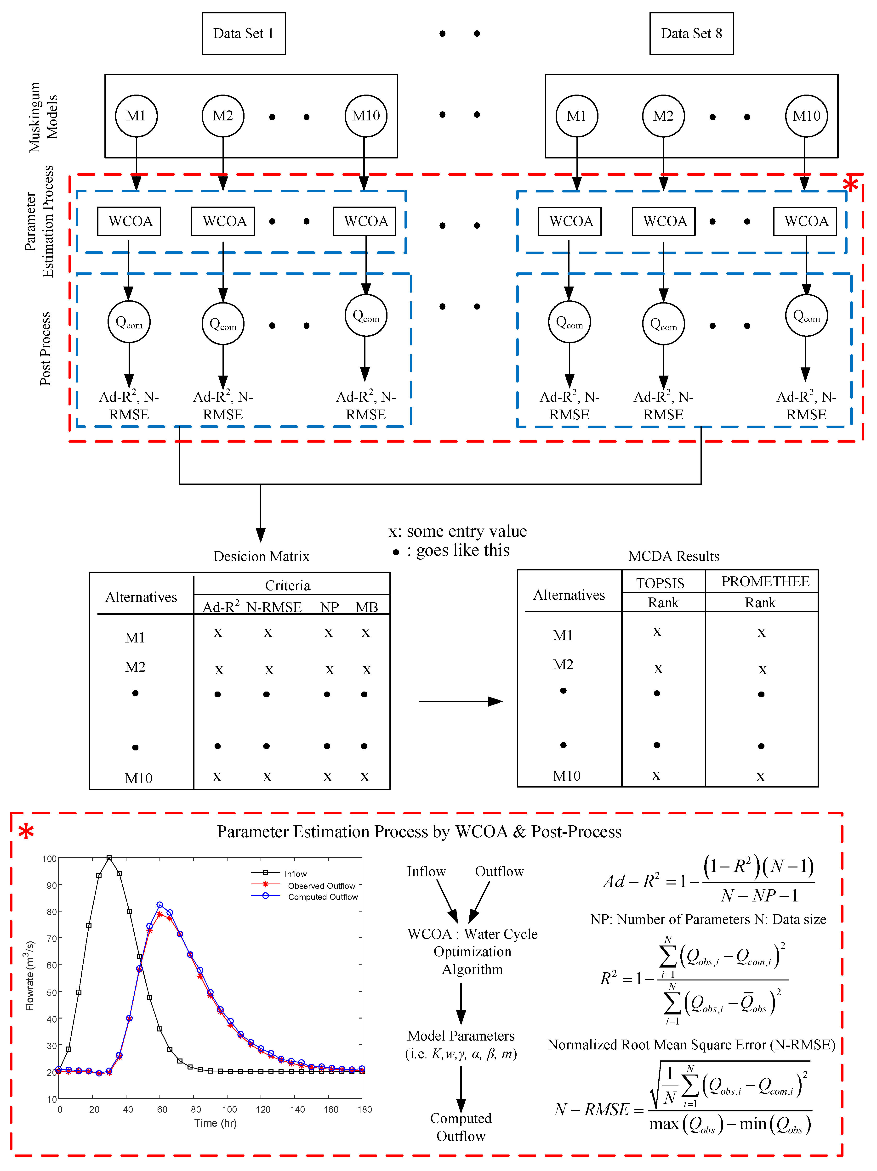
	M10	1000	0.9450	−1.1817	5.0	5.1915	0.1637	0.9390	3160.90	0.9921	0.0251	8.48

. During the optimization process, the WCOA was run 10 times for each flood dataset in order to obtain more reliable model parameters with accurate ranges. For instance, when the model parameters of M1 were determined by using dataset 1 (DS1), 10 possible candidate solutions were retrieved by the WCOA. Although the estimated model parameters could be very close to each other for each trial, the estimated parameter set with the smallest cost function value among the candidate solutions was noted. Thus, the error metrics for each model were computed, as given in Table A1. The same process was repeated to obtain the error metrics for the remaining models.

According to the findings presented in Table A1, models M7, M8, M9, and M10 yielded highly accurate predictions considering the error metrics of $Ad-R^2$ (>0.999) and N-RMSE (<0.01) for DS1 as the smooth single peak (SSP) dataset. For the dataset DS2, which shares similar attributes to DS1, it is worth noting that, in addition to the models mentioned previously, models M2, M3, and M5 also exhibit considerable predictive performance with respect to the aforementioned metrics of $Ad-R^2$ (>0.999) and N-RMSE (<0.01). For the non-smooth single peak (NSP) datasets (DS3 and DS4), when evaluated with both metrics ($Ad-R^2$ > 0.98 and N-RMSE < 0.31), models M9 and M10 provide the best results, but it is observed that the prediction capacity of these models decreases when compared to those in SSP datasets. When examining the DS5 dataset, which is of the multi-peak (MP) type, it was observed that all models, except for the M4 model, provided relatively good prediction results. Another dataset (DS6) of the same type (MP) showed that the models between M5 and M10 performed well. However, in these datasets (DS5 and DS6), the performance of the M5, M9, and M10 models stands out compared to others when considering both error metrics. Finally, for the datasets referred to as irregular (DS7 and DS8) in this study, the M5, M9, and M10 models were consistently ranked as the top three performers among the 10 models evaluated in both $Ad-R^2$ ($Ad-R^2$ > 0.99) and N-RMSE (N-RMSE < 0.015 for DS7 and N-RMSE < 0.025 for DS8). This situation was also observed for the estimation performance of the models realized in the MP type.

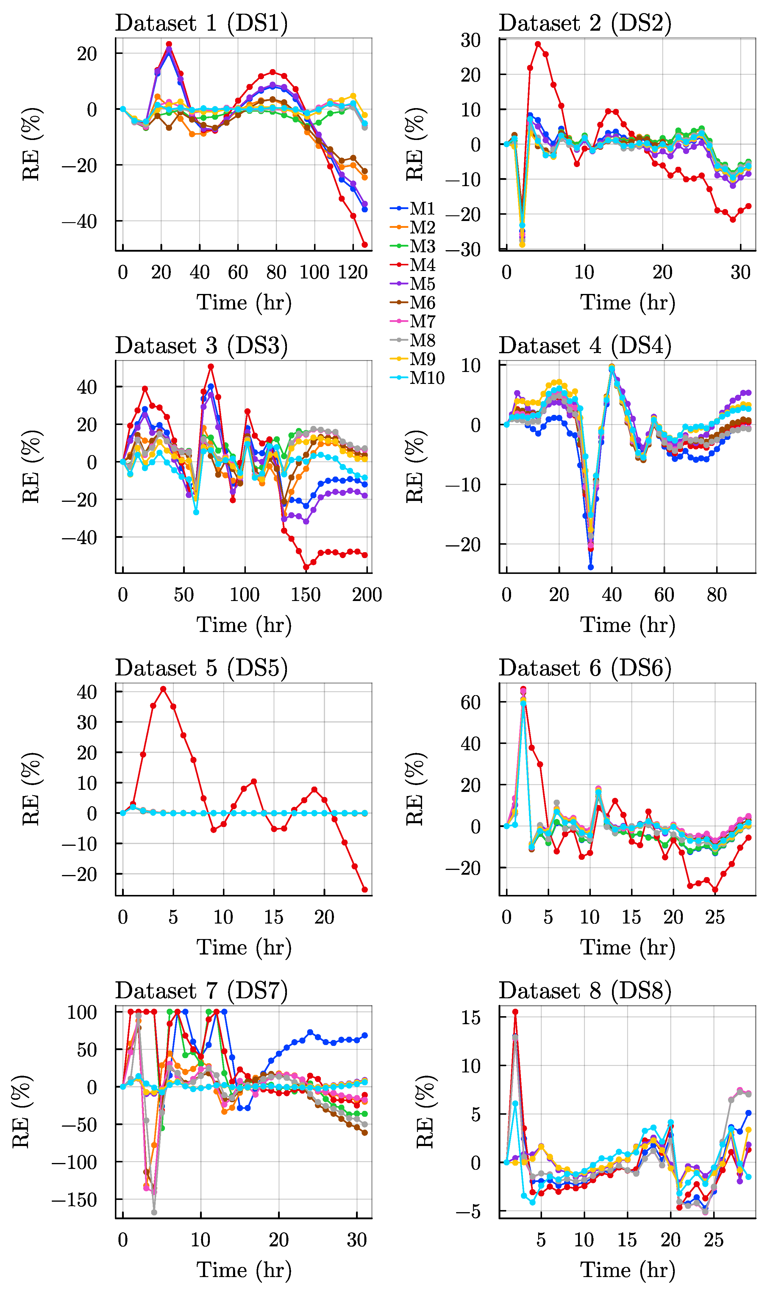
Figure 3 also depicts the relative percentage error of each model over the given flood duration for each dataset. For the SSP-type datasets (DS1 and DS2), all methods could achieve better parameter estimation performance within a certain error tolerance. The falling and the rising limbs of each hydrograph for M4 show an increase in the error percentages and this error is even more pronounced in the falling limbs of the hydrographs, especially for the SSP type. In addition, a similar pattern can be observed for the NSP-type datasets (DS3 and DS4). Likewise, the relative errors of the models, except for model M4, were very small for DS5, that belongs to the MP-type dataset category. However, all methods, in general, gave reasonable estimation results for DS6, that was categorized as an MP-type dataset. Models M1, M3, and M4 were not able to produce the model parameters satisfying a good performance for DS7 while the remaining ones successfully estimated the model parameters. For DS8 as an irregular dataset type, the model parameters of all methods could be easily identified by the WCOA.

The Wilson river flood dataset (DS1) has been studied by several researchers. The reported SSE values (in (m³/s)²) for this dataset were obtained as 39.8 by [44], 17.55 by [45], 9.82 by [11], 7.67 by [2], 5.124 by [46], 4.11 by [47], 4.04 by [25], 1.92 by [31], 1.092 by [48], 0.799 by [49], and 0.65 by [50]. In this study, the SSE value for DS1 with the WCOA was found to be 7.66. Moreover, the proposed model (M10) achieved an SSE value of 4.09. The range of SSE values reported by different researchers suggests that there may be considerable variability in flood modeling results for this dataset, depending on the specific optimization algorithm and routing approach used. For instance, the SSE value of model M7 in this study (with the four-parameter non-linear model proposed by [2]) was calculated as 7.67, while the same metric was found to be 9.82 for model M9 (with the four-parameter non-linear model by [11]). Although these two models have the same number of model parameters, the reported SSE values are different because the researchers used different routing approaches and optimization algorithms as well. Similar findings can also be drawn for other datasets used in this study. For the Viessman and Lewis flood dataset (DS5), the reported SSE values were 71,708 in [45], 65,324 in [44], 28,855 in [50], and 8449 in [49]. However, the implemented routing model with the WCOA in this study provided notably smaller SSE values using the examined models except for M4, as shown in Table A1. It is quite remarkable that the SSE value of model M1 (with the two-parameter linear model proposed by [5]) was 14.53, while a model proposed by [49] with 12 parameters yielded an SSE value of 8449. However, comparing the reported results in the literature directly (without taking into account the applied routing approaches and optimization methods) can be misleading in interpreting which model exhibited a better estimation performance.

In summary, this exercise reveals that the WCOA is able to show a very competitive estimation performance when compared to the reported literature. Thus, the WCOA can be regarded as a viable algorithm with the outlined routing approach. These findings also suggest that the particular models are effective in capturing the outflow patterns in these datasets.

To interpret the performance of the models in Table A1, the models were ordered according to their $Ad-R^2$ and N-RMSE. Considering $Ad-R^2$ values, the rank score was then assigned to each model such that ranking starts from 1 for the model having the highest $Ad-R^2$ value and successively continues to the rank value of 10. For N-RMSE values, the rank score starts from 1 for the smallest N-RMSE value, as shown in

Table 3. Ranking results of models for criteria $Ad-R^2$ and N-RMSE.

$\mathit{A}\mathit{d}-{\mathit{R}}^2$
	SSP			NSP			MP			Irregular			Overall
Model	DS1	DS2	AR	DS3	DS4	AR	DS5	DS6	AR	DS7	DS8	AR	AR
M1	8	9	8.5	9	10	9.5	7	8	7.5	10	4	7	8.125
M2	7	6	6.5	7	7	7	8	4	6	7	5	6	6.375
M3	5	8	6.5	5	6	5.5	9	9	9	8	6	7	7
M4	10	10	10	10	9	9.5	10	10	10	9	10	9.5	9.75
M5	9	7	8	8	4	6	1	1	1	2	2	2	4.25
M6	6	3	4.5	6	8	7	6	5	5.5	4	7	5.5	5.625
M7	3	2	2.5	3	5	4	4	6	5	5	8	6.5	4.5
M8	2	1	1.5	4	3	3.5	5	7	6	6	9	7.5	4.625
M9	4	4	4	2	2	2	2	2	2	3	1	2	2.5
M10	1	5	3	1	1	1	3	3	3	1	3	2	2.25
N-RMSE
M1	9	9	9	9	10	9.5	9	9	9	10	9	9.5	9.25
M2	7	6	6.5	7	8	7.5	7	7	7	7	6	6.5	6.875
M3	5	8	6.5	5	6	5.5	8	8	8	8	7	7.5	6.875
M4	10	10	10	10	9	9.5	10	10	10	9	10	9.5	9.75
M5	8	7	7.5	8	5	6.5	3	2	2.5	3	2	2.5	4.75
M6	6	4	5	6	7	6.5	6	5	5.5	4	8	6	5.75
M7	3	2	2.5	4	4	4	5	6	5.5	6	5	5.5	4.375
M8	2	1	1.5	3	3	3	4	4	4	5	4	4.5	3.25
M9	4	5	4.5	2	2	2	2	3	2.5	2	1	1.5	2.625
M10	1	3	2	1	1	1	1	1	1	1	3	2	1.5

. Furthermore, the averaged rank (AR) of each model was given for the datasets previously categorized as SSP, NSP, MP, and irregular. Based on the overall AR value of $Ad-R^2$ and N-RMSE in Table 3, the best two models were found to be M9 and M10, whereas the worst two models were noted to be M1 and M4. When the results are analyzed according to the hydrograph type, model M4 shows the worst performance with a rate of 75% (six times it was assigned with a rank score of 10 among the eight datasets) for both criteria. Although this model has a physical sense evolving from the Manning equation, forcing the model with a constant exponent (m = 3/5) decreases the performance in the calculations. This remark is also supported by the relative error results, presented in Figure 3. However, the best model is not the same for all hydrograph types. Although half of the datasets, more specifically four datasets for the $Ad-R^2$ criterion and five datasets for the N-RMSE criterion, have superior results with model M10; models M8, M5, and M9 are ranked as the best for the hydrograph types of SSP, MP, and irregular, respectively.

Considering Table A1 and Table 3, any comparison between the error metrics could be insufficient to form a solid judgment. Therefore, a comprehensive assessment was needed to compare the capabilities of the models. To apply the methodologies of MCDA outlined previously, the decision matrix for each hydrograph type was set as listed in

Table 4. Decision matrix for four hydrograph types: SSP, NSP, MP, and irregular.

SSP					NSP
Model	$Ad-R^2$	N-RMSE	NP	MB	Model	$Ad-R^2$	N-RMSE	NP	MB
M1	8.5	9	2	1	M1	9.5	9	2	1
M2	6.5	6.5	3	0	M2	7	7	3	0
M3	6.5	6.5	3	0	M3	5.5	5	3	0
M4	10	10	2	1	M4	9.5	9	2	1
M5	8	7.5	3	1	M5	6	6	3	1
M6	4.5	5	4	0	M6	7	6	4	0
M7	2.5	2.5	4	0	M7	4	4	4	0
M8	1.5	1.5	5	0	M8	3.5	3	5	0
M9	4	4.5	4	0	M9	2	2	4	0
M10	3	2	6	0	M10	1	1	6	0
MP					Irregular
Model	$Ad-R^2$	N-RMSE	NP	MB	Model	$Ad-R^2$	N-RMSE	NP	MB
M1	7.5	9	2	1	M1	7	9.5	2	1
M2	6	7	3	0	M2	6	6.5	3	0
M3	9	8	3	0	M3	7	7.5	3	0
M4	10	10	2	1	M4	9.5	9.5	2	1
M5	1	2.5	3	1	M5	2	2.5	3	1
M6	5.5	5.5	4	0	M6	5.5	6	4	0
M7	5	5.5	4	0	M7	6.5	5.5	4	0
M8	6	4	5	0	M8	7.5	4.5	5	0
M9	2	2.5	4	0	M9	2	1.5	4	0
M10	3	1	6	0	M10	2	2	6	0

. The results presented in

Table 5. Ranking results (starting from the best model) and scores of TOPSIS and PROMETHEE for three scenarios and four hydrograph types.

Dataset Type	Scenario 1				Scenario 2				Scenario 3
	TOPSIS		PROMETHEE		TOPSIS		PROMETHEE		TOPSIS		PROMETHEE
	Model	$\mathit{\chi }$	Model	$\mathit{\xi }$	Model	$\mathit{\chi }$	Model	$\mathit{\xi }$	Model	$\mathit{\chi }$	Model	$\mathit{\xi }$
SSP	8	0.5475	8	0.1251	8	0.5971	8	0.1693	8	0.6970	8	0.2577
	5	0.5398	7	0.1157	7	0.5779	7	0.1464	7	0.6730	7	0.2078
	7	0.5311	5	0.0507	10	0.5477	10	0.0353	10	0.6481	10	0.1245
	1	0.5116	1	0.0413	5	0.4954	5	0.0124	9	0.5656	9	0.0477
	10	0.4981	10	−0.0093	9	0.4918	9	0.0092	6	0.5266	6	0.0020
	4	0.4684	9	−0.0101	1	0.4622	1	−0.0105	5	0.4087	5	−0.0642
	9	0.4536	6	−0.0461	6	0.4613	6	−0.0301	2	0.3850	1	−0.1141
	6	0.4268	4	−0.0485	4	0.4179	4	−0.1085	3	0.3850	2	−0.1165
	2	0.3525	2	−0.1094	2	0.3637	2	−0.1118	1	0.3626	3	−0.1165
	3	0.3525	3	−0.1094	3	0.3637	3	−0.1118	4	0.3158	4	−0.2284
NSP	5	0.5939	5	0.1586	10	0.5812	9	0.1856	10	0.6834	10	0.2618
	10	0.5307	9	0.1516	9	0.5771	10	0.1529	9	0.6723	9	0.2536
	9	0.5303	10	0.0985	5	0.5555	5	0.1301	8	0.5904	8	0.0975
	1	0.4693	7	0.0078	8	0.5037	8	0.0320	7	0.5459	5	0.0730
	4	0.4693	8	−0.0007	7	0.4761	7	0.0288	5	0.4836	7	0.0706
	8	0.4593	1	−0.0126	1	0.4188	3	−0.0333	3	0.4293	3	−0.0250
	7	0.4396	4	−0.0126	4	0.4188	1	−0.0693	1	0.3166	6	−0.1810
	3	0.3804	3	−0.0375	3	0.3973	4	−0.0693	4	0.3166	1	−0.1827
	2	0.2849	2	−0.1633	6	0.2835	2	−0.1706	6	0.3023	4	−0.1827
	6	0.2730	6	−0.1899	2	0.2814	6	−0.1869	2	0.2747	2	−0.1851
MP	5	0.8853	5	0.4671	5	0.8856	5	0.4667	5	0.8863	5	0.4657
	9	0.5361	9	0.1207	9	0.5821	9	0.1519	9	0.6743	9	0.2142
	1	0.5161	1	0.0883	10	0.5612	10	0.0593	10	0.6577	10	0.1525
	10	0.5125	10	0.0127	1	0.4687	1	0.0407	8	0.4792	7	−0.0451
	4	0.4556	4	−0.0306	8	0.4199	7	−0.0704	7	0.4670	1	−0.0543
	7	0.3898	7	−0.0830	7	0.4174	4	−0.0889	6	0.4454	8	−0.0651
	8	0.3865	6	−0.1000	4	0.4054	6	−0.0889	1	0.3757	6	−0.0667
	6	0.3746	2	−0.1054	6	0.4000	8	−0.1074	2	0.3708	2	−0.1114
	2	0.3450	8	−0.1285	2	0.3541	2	−0.1074	4	0.3047	4	−0.2056
	3	0.2444	3	−0.2412	3	0.2319	3	−0.2556	3	0.2072	3	−0.2843
Irregular	5	0.8966	5	0.4697	5	0.8995	5	0.4694	5	0.9051	5	0.4690
	9	0.5433	9	0.1954	9	0.5912	9	0.2333	9	0.6900	9	0.3093
	1	0.5349	1	0.0611	10	0.5528	10	0.1014	10	0.6574	10	0.2016
	10	0.5020	10	0.0513	1	0.4872	1	0.0111	6	0.4213	1	−0.0889
	4	0.4896	4	−0.0407	4	0.4387	2	−0.0972	7	0.3986	6	−0.0910
	2	0.3515	2	−0.0961	6	0.3743	4	−0.1000	8	0.3979	2	−0.0995
	6	0.3494	6	−0.1191	2	0.3634	6	−0.1097	1	0.3919	7	−0.1185
	7	0.3342	7	−0.1407	7	0.3566	7	−0.1333	2	0.3872	8	−0.1634
	8	0.3193	3	−0.1750	8	0.3475	3	−0.1833	4	0.3344	3	−0.2000
	3	0.2965	8	−0.2058	3	0.2956	8	−0.1917	3	0.2939	4	−0.2185

cover the ranking obtained from the MCDA tools considering four hydrograph types under three scenarios. To this end, the average rank values for $Ad-R^2$ and N-RMSE were employed as decisive criteria for each dataset. The performance of a model can be evaluated using two metrics, and in this context, a lower value assigned implies better performance. Specifically, the metrics are inversely proportional to the model’s effectiveness, meaning that a decrease in the assigned value indicates an improvement in the model’s performance. Therefore, the aforementioned two metrics were considered as non-beneficiary (minimized) criteria. The number of parameters (NP) for a model could be again considered as a decisive criterion. As listed in Table 1, the NP could indicate the models’ complexity. A model containing fewer parameters may be more desirable than a model with a larger number of parameters. Thus, NP was a non-beneficiary (minimized) criterion. Finally, the dimensional consistency of a model was labeled as the model background (MB) criterion. A model constructed using physical-based parameters was deemed more realistic compared to a model that employed additional parameters solely for improving the fitting accuracy. In this criterion, a binary entry of 1 was assigned to physically sound models, while models containing non-physical parameters solely used for fitting purposes were assigned a binary value of 0, as shown in Table 4. Therefore, the MB was assigned as a beneficiary (maximized) criterion.

3.2. Multi-Criteria Decision Analysis (MCDA) Results

To apply MCDA tools effectively, it is essential to identify the weight of each criterion. To achieve this, three distinct weight scenarios were designed. In scenario 1, the weights assigned to the $Ad-R^2$, N-RMSE, NP, and MB criteria were 0.275, 0.275, 0.225, and 0.225, respectively. This scenario implies that the weights for the error metrics criteria (55%) are slightly higher than those for the remaining criteria (45%). Therefore, the results from scenario 1 were expected to provide a balanced ranking of the employed models taking into account the implemented criteria. In scenario 2, weights of 0.3, 0.3, 0.2, and 0.2 were assigned to the $Ad-R^2$, N-RMSE, NP, and MB criteria, respectively. The objective of scenario 2 was to observe the impact of increasing the weights for the error metrics on the ranking. Finally, scenario 3 was designed to assign more weight to the error metric criteria (0.35 each), while the remaining NP and MB criteria were given weights of 0.15 each. Through this assessment, these scenarios can provide a better understanding of how different the weight distribution to each criterion may affect the ranking of the models implemented.

Both TOPSIS and PROMETHEE identified model M8 (a non-linear model with five parameters proposed by [10]) as the most suitable model for the hydrograph type of SSP in all scenarios. With the NSP hydrograph type, model M5 (a linear model with three physical-based parameters) was found to be the best model according to the aforementioned criteria for scenario 1, as determined by both tools. However, in scenario 3, where the error performance was dominant, model M10 (non-linear model with six parameters) was identified as the best alternative model among the comparison poll. It should be noted that model M10 was identified as the best performing model based on the $Ad-R^2$ and N-RMSE criteria as shown in Table 4. However, the ranking order may shift due to the influence of the NP and MB criteria, which can cause model M5 to move from a lower position to the top, as observed in scenario 1. This underscores the importance of using a multi-criteria decision analysis approach to ensure a fair and comprehensive evaluation of the capabilities of the examined models. For the MP and irregular hydrograph types, the application of both MCDA tools consistently identified the M5 model and its non-linear variant M9 (with four parameters) as the best and second-best models, respectively, across all scenarios. However, a highly competitive model, M10, was observed to have superior performance based on its $Ad-R^2$ and N-RMSE values as listed in Table 4 for the MP and irregular types. Notably, the ranking of the models was observed to be sensitive to the weight scenarios utilized in this study, as demonstrated by the varying influence of the NP and MB criteria. As observed from Table 5, M1, the classical linear model with two parameters, showed a notable performance when model simplicity and background were preferable, as aimed for in scenario 1. Both MCDA tools determined the fourth ranking place for the SSP, and third place for the MP and irregular types. However, fourth place can be obtained by TOPSIS, whereas PROMETHEE put it in sixth place when the NSP-type datasets are employed. All in all, model M1 is still a viable model if the complexity as a decisive criterion is taken into account by the practitioners. Furthermore, the data characteristic may affect the efficiency of the models. Model M8 was found to be the best model for the SSP, whereas its capability dramatically varied for the MP and irregular hydrograph types under the scenarios implemented. As an additional evaluation, a new decision matrix was created using the overall average AR scores of eight flood events (shown in the last column of Table 3) to eliminate any potential impact of hydrograph type, as given in

Table 6. MCDA results of all flood events. (a) Decision matrix obtained from 8 flood events and (b) corresponding scores of TOPSIS and PROMETHEE for three scenarios.

(a)
	Model		$Ad-R^2$		N-RMSE		NP		MB
	M1		8.125		9.25		2		1
	M2		6.375		6.875		3		0
	M3		7		6.875		3		0
	M4		9.75		9.75		2		1
	M5		4.25		4.75		3		1
	M6		5.625		5.75		4		0
	M7		4.5		4.375		4		0
	M8		4.625		3.25		5		0
	M9		2.5		2.625		4		0
	M10		2.25		1.5		6		0
(b)
Scenario 1				Scenario 2				Scenario 3
TOPSIS		PROMETHEE		TOPSIS		PROMETHEE		TOPSIS		PROMETHEE
Model	$\chi$	Model	$\xi$	Model	$\chi$	Model	$\xi$	Model	$\chi$	Model	$\xi$
5	0.7539	5	0.2912	5	0.7346	5	0.2747	5	0.7008	5	0.2418
9	0.5271	9	0.1287	9	0.5742	9	0.1606	10	0.6722	9	0.2244
1	0.5201	10	0.0556	10	0.5687	10	0.1061	9	0.6711	10	0.2071
10	0.5179	1	0.0292	8	0.4946	7	0.0010	8	0.5833	8	0.0431
4	0.4821	7	−0.0176	7	0.4804	8	−0.0146	7	0.5558	7	0.0382
8	0.4498	8	−0.0435	1	0.4707	1	−0.0237	6	0.4473	6	−0.0849
7	0.4420	4	−0.0556	4	0.4313	6	−0.1045	2	0.3717	1	−0.1295
6	0.3686	6	−0.1144	6	0.3959	4	−0.1162	1	0.3701	2	−0.1352
2	0.3429	2	−0.1241	2	0.3527	2	−0.1278	3	0.3420	3	−0.1676
3	0.3248	3	−0.1495	3	0.3306	3	−0.1556	4	0.3278	4	−0.2374

. Once again, the M5 model and its non-linear variant M9 were found to be the superior models for scenarios 1 and 2, as indicated in the decision matrix presented in Table 3. In scenario 3, where error metrics were dominant, TOPSIS ranked model M9 in the third place, while PROMETHEE placed it in second place.

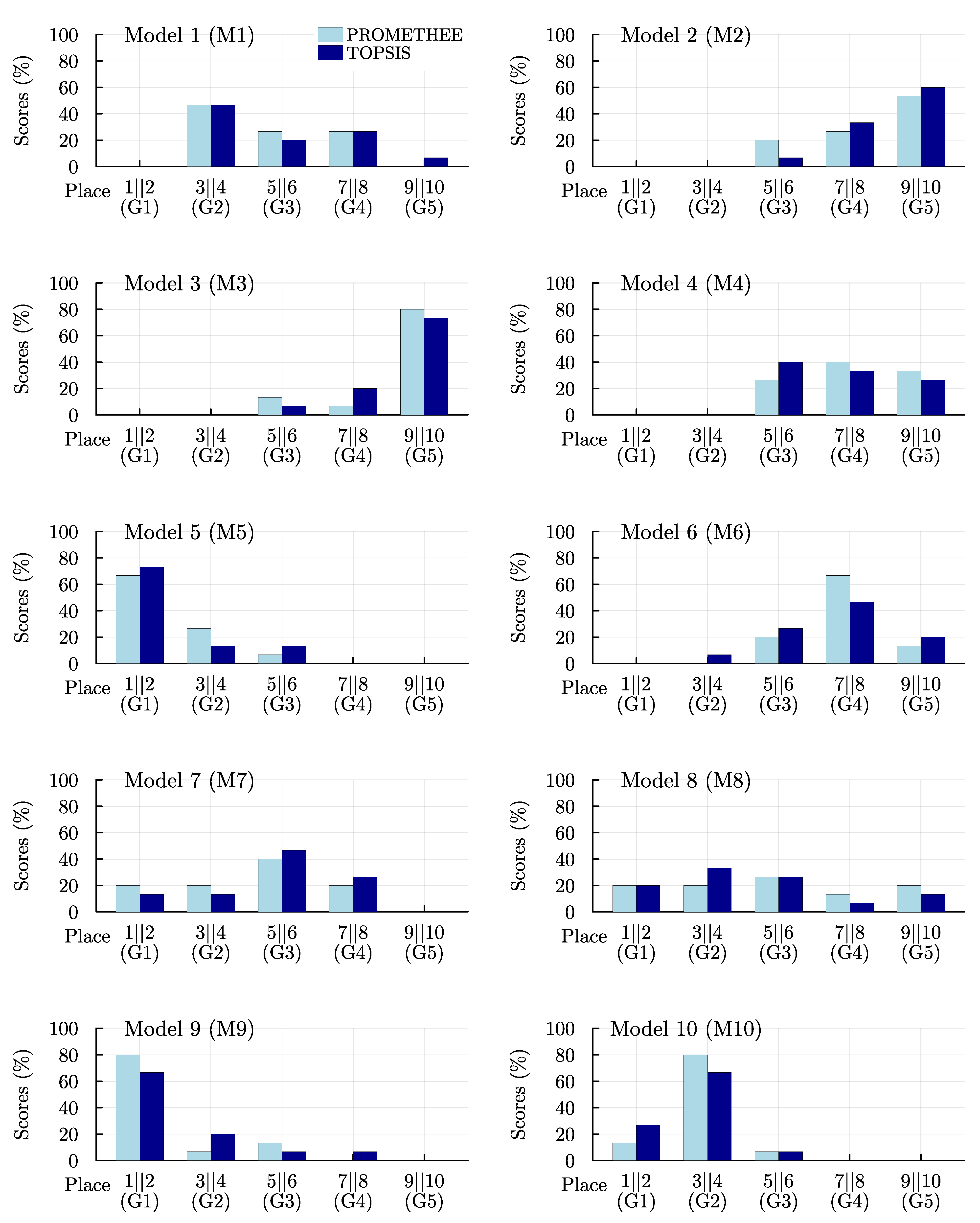
As mentioned earlier, Table 5 presents the results of four different hydrograph types, while Table 6 displays the outcomes based on the average AR values of eight distinctive flood events. To facilitate the interpretation of the results for each model, the ranking places of each model can be categorized into five main groups: the first or the second place (denoted as 1||2) in group 1 (G1), the third or the fourth place (3||4) in group 2 (G2), the fifth or the sixth place (5||6) in group 3 (G3), the seventh or the eighth place (7||8) in group 4 (G4), and the ninth or the tenth place (9||10) in group 5 (G5), as illustrated in Figure 4. In other words, there are 15 possible cases (four for hydrograph types and one aggregated evaluation for all datasets by three scenarios) provided by each MCDA tool for each model. For instance, in the case of SSP using TOPSIS, the ranking places of the M1 model were found to be the fourth place in scenario 1, sixth place in scenario 2, and ninth place in scenario 3. This procedure was carried out for each model and the implemented cases. The ranking places were noted for each model among the implemented cases and subsequently categorized as explained. For example, the performance of model M1 was categorized as 0% in G1, 46.6% (7 occurrences out of 15) in G2, 20% (3 out of 15) in G3, 26.6% (4 out of 15) in G4, and 6.6% (1 out of 15) in G5, as shown in Figure 4. As also seen in Figure 4, model M5 was able to produce a superior performance to complete the comparison within the first and the second ranking places (G1) with scores of 73.3% by TOPSIS and 66.6% by PROMETHEE. Similarly, model M9 can be evaluated as an identical competitor model regarding its scores in G1, which were 66.6% by TOPSIS and 80% by PROMETHEE. Apart from these models, model M10 can give the highest success rate for the third and fourth places (G2), which were 66.6% by TOPSIS and 80% by PROMETHEE. For the G2 category, model M1 showed a notable performance, with equal success scores of 46.6% by TOPSIS and PROMETHEE. 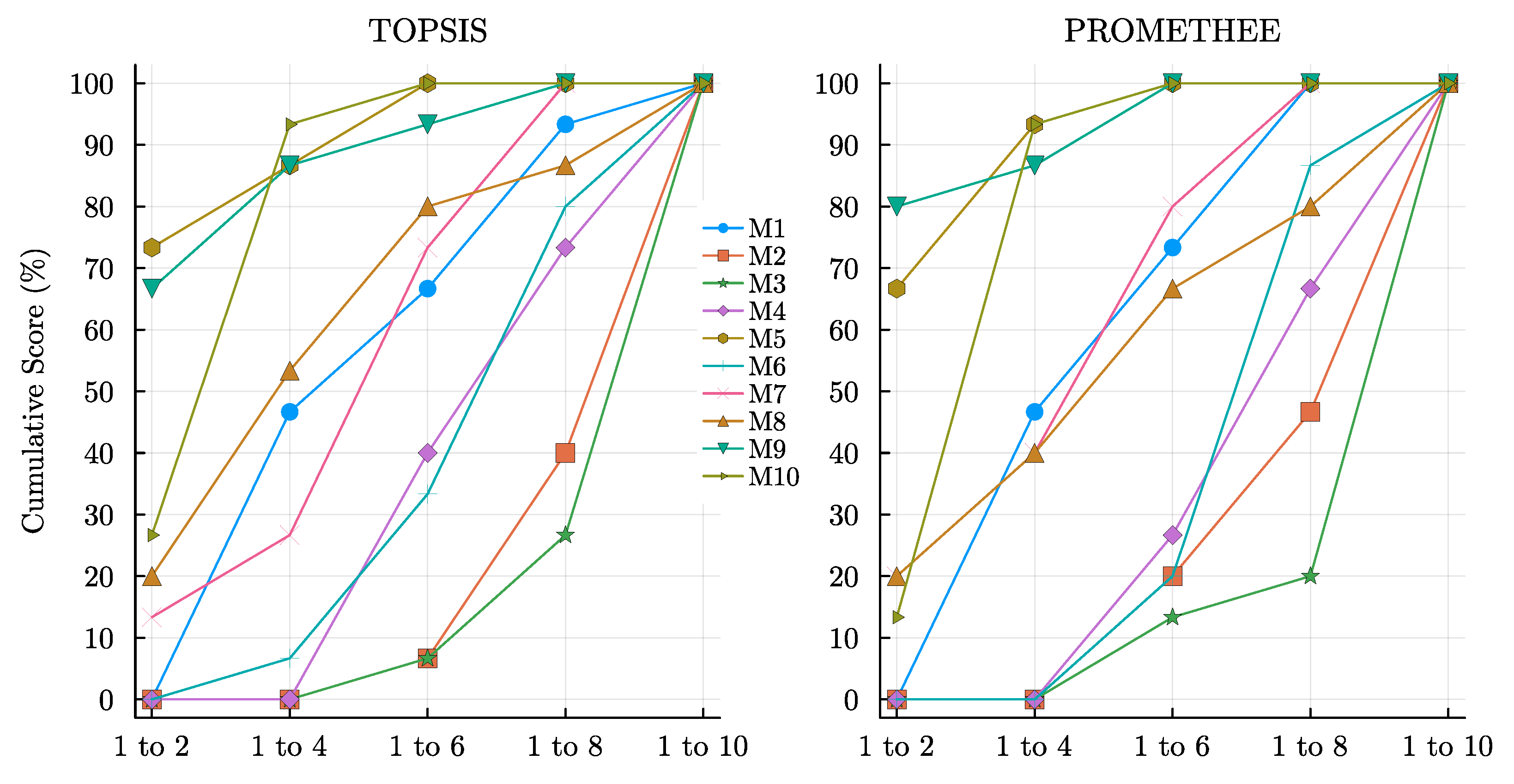For an alternative interpretation of Figure 4, the success rate for each ranking place category is cumulatively shown in Figure 5 in order to understand which model stands out. As a result of the analyses conducted using both MCDA tools, models M5, M9, and M10 emerge as the top performers among the flood routing models in the comparison pool, as illustrated in Figure 5.

3.3. Comparison of MCDA Tools

In this study, two outranking MCDA tools, TOPSIS and PROMETHEE, were employed to evaluate the performance of different Muskingum models under the aforementioned criteria. TOPSIS and PROMETHEE are widely used in decision-making processes due to their ability to handle complex decision problems [51]. In general, any MCDA method can develop a different series of rankings for the same problem depending on the strategy and mathematical background of MCDA implemented. TOPSIS is sensitive to the weights assigned to the criteria and ignores the interrelationships between the criteria [52]. PROMETHEE, on the other hand, generates a pairwise comparison matrix to assess the relative importance of each criterion [53]. However, it is sensitive to the choice of preference function and decision threshold used [54]. Therefore, selecting the appropriate MCDA method depends on the specific problem being addressed and the characteristics of the data being evaluated [55,56,57].

To analyze the differences in rankings obtained from TOPSIS and PROMETHEE, a consistency rate (CR), which is the percentage of cumulative differences of the model ranked from the same case for both MCDA tools, was defined. As observed from Table 5, both MCDA tools ranked models M8, M1, M10, M2, and M3 in the 1st, 4th, 5th, 9th, and 10th ranking places, respectively, in scenario 1. Thus, the CR of both tools for the SSP was realized as 50% (5 out of 10) in scenario 1, 100% in scenario 2 and 70% (7 out of 10) in scenario 3, which yields an average of 73.3% overall. For the NSP type, the CR was observed to be 40%, 30%, and 50% for scenarios 1, 2, and 3, respectively. It is noteworthy that the CR is 70% in scenario 1, 60% in scenario 2, and 60% in scenario 3 for the MP type, whereas the CR values of the irregular type were 80%, 50%, and 30% in scenarios 1, 2, and 3, respectively. This analysis is denoted CR(0) and depicted in Figure 6. The plus (+) values in Figure 6 indicate that TOPSIS ranks the model higher compared to PROMETHEE, while the minus (−) values indicate the opposite condition. Furthermore, the CR was recomputed in such a way that $\pm 1$ rank difference between the MCDA tools was tolerated and denoted as CR(1), shown in a gray color in Figure 5. Considering the CR(1) values, both MCDA tools are in a high accordance for almost all cases implemented in this study. Thus, this analysis highlights the effectiveness of these MCDA tools in providing reliable model rankings.

4. Summary and Conclusions

In this research, an extensive analysis was conducted on the estimation capabilities of several commonly used Muskingum models in flood routing using two different MCDA methods, namely, TOPSIS and PROMETHEE, with the help of eight distinct flood datasets reported in the literature. The estimation performance of the flood routing models may depend on diverse factors such as the model parameters, which can be either physical-based or empirical ones that minimize the error between the output flow calculated by the flood routing methods and the observed output flow, the effectiveness of the applied optimization method, and the numerical flood routing procedure with implicit or explicit schemes. The results demonstrated that not every proposed model performed well on every dataset. Apart from utilizing error metrics to assess the estimation performance of the models, it is also crucial to thoroughly examine how each model performs with varying degrees of success on different datasets. The key findings can be summarized as follows:

(1)

The WCOA used in this study showed a viable ability in parameter estimation when compared to other algorithms used in similar studies.

(2)

The criteria, $Ad-R^2$ and N-RMSE, revealed that the non-linear models M9 and M10 (with four and six parameters) showed better predictive performance than the rest of the models on all datasets. However, the temporal distribution of the relative error showed diversity in defining the best routing models overall. Such findings indicate the importance of the criteria in the selection of the proper model and parameters.

(3)

The model performances were also assessed by clustering the hydrograph types, smooth single peak (SSP), non-smooth single peak (NSP), multi-peak (MP), and irregular. According to the average of the ranked criteria overall, models M9 and M10 showed the best performance according to the error metric criteria, including $Ad-R^2$ and N-RMSE. For hydrograph types, the definition of the best model showed some variability, the proposed model M10 showed better performance for the majority of the datasets by considering these criteria.

(4)

To obtain a more rigid conclusion about defining the best model, two different multi-criteria decision analysis (MCDA) tools were applied by using two additional criteria: the number of model parameters (NP), which indicates the model complexity; and the model background (MB), which characterizes the model parameters as either physical-based or empirical, with the purpose of improving the fitting.

(5)

The effects of the relative importance of each criterion were investigated by assigning three different weight scenarios in both tools, TOPSIS and PROMETHEE. The most outstanding remark is the compatibility of both tools in all scenarios, giving similar model results in the rankings. However, it was seen that the governing factor in defining the best model depends on the scenario selection. In scenario 1, where additional criterion weights are balanced when compared to the other scenarios, physical-based models were more successful. However, there is a variety of ways to define the best model for hydrograph types. Model M5, a physically sound model, showed the best results for MP and irregular hydrograph types, whereas models M8 and M10, empirical models with a high number of parameters, showed better results compared to the rest of the models for the SSP and NSP types. Such outcomes may indicate that the routing application in complex hydrographs that have more than one peak with irregular limps can be assessed better using physical-based routing models that have fewer parameters.

(6)

The MCDA in a single pool ignoring the clustering of hydrograph types showed that model M5 had the greatest score in the rankings. Moreover, the cumulative score evaluation of 10 Muskingum models that cover the cumulative percentages of the model ranking place shows that models M5, M9, and M10 have the leading results with scores of 85% in the top four ranking places for both tools, TOPSIS and PROMETHEE. Such a result can be beneficial for researchers in choosing the proper routing models in their area of interest.

(7)

There are a variety of Muskingum models applied in the literature. Within this study, the success of the models was assessed concerning the model parameters (complexity), model constructions (empirical or physical), error metrics, and hydrograph types. The most suitable model, model M5, showed that the use of physical-based models with fewer parameters among the possible model sets studied here, may be beneficial.

(8)

Any MCDA method can inherently generate a different ranking for the problem of interest. Although the tools used in this study have different capabilities in terms of relating the criteria and being sensitive to the weights of the criteria, their results are compatible with each other. This outcome reveals the independence of the criteria and stability of the weights in application. This finding was also testified by the consistency rates (CR) that involve the proximity of model rankings for each scenario and hydrograph types performed for both tools.

In this study, although a comprehensive assessment was completed by involving the factors aforementioned above, there is a limited number of datasets. Future studies may improve on the presented results by using new flow datasets. The findings in this work are the result of eight different flood case studies reported previously in the literature. Since the workflow given here does not depend on a specific region, it can be applied to other regions as well. Considering all the events, it can be generalized that achieving a successful running model depends on the purpose of the work and the hydrograph characteristics. Although the purpose of the work that covers the model complexity and the importance of correlation can be decided before a flood happens, estimating the hydrograph type is a challenging task. Such an issue, at least the prediction of the inflow hydrograph, may be handled by implementing hydrologic models that can work with numerical weather prediction products. In addition to remote sensing products with proper hydrologic models, field and laboratory experiments should be made in the future that may provide a broad generalization in the selection of the best routing model.

References

1. Afzali, S.H. Variable-parameter Muskingum model. Iran. J. Sci. Technol. Trans. Civ. Eng. 2016, 40, 59–68. [Google Scholar] [CrossRef]
2. Easa, S.M. New and Improved Four-Parameter Non-Linear Muskingum Model. Proc. Inst. Civ. Eng. Water Manag. 2014, 167, 288–298. [Google Scholar] [CrossRef]
3. Gąsiorowski, D.; Romuald, S. Dimensionally Consistent Nonlinear Muskingum Equation. J. Hydrol. Eng. 2018, 23, 04018039. [Google Scholar] [CrossRef]
4. Bai, T.; Wei, J.; Yang, W.; Huang, Q. Multi-objective parameter estimation of improved Muskingum model by wolf pack algorithm and its application in Upper Hanjiang River, China. Water 2018, 10, 1415. [Google Scholar] [CrossRef] [Green Version]
5. McCarthy, G.T. The unit hydrograph and flood routing. In Conference of North Atlantic Division; US Army Corps of Engineers: Washington, DC, USA, 1938. [Google Scholar]
6. Chow, V.T. Open-Channel Hydraulics; McGraw-Hill: New York, NY, USA, 1959. [Google Scholar]
7. Gill, M.A. Flood routing by the Muskingum method. J. Hydrol. 1978, 36, 353–363. [Google Scholar] [CrossRef]
8. O’donnell, T. A Direct Three-Parameter Muskingum Procedure Incorporating Lateral Inflow. Hydrol. Sci. J. 1985, 30, 479–496. [Google Scholar] [CrossRef] [Green Version]
9. Gavilan, G.; Houck, M.H. Optimal Muskingum river routing. In Proceedings of the ASCE Computer Applications in Water Resources, Buffalo, NY, USA, 10–12 June 1985; American Society of Civil Engineers: New York, NY, USA, 1985; pp. 1294–1302. [Google Scholar]
10. Vatankhah, A.R. Discussion of parameter estimation of the nonlinear Muskingum flood routing model using a hybrid harmony search algorithm by Halil Karahan, Gurhan Gurarslan, and Zong Woo Geem. J. Hydrol. Eng. 2014, 19, 839–842. [Google Scholar] [CrossRef]
11. Karahan, H.; Gurarslan, G.; Geem, Z.W. A New Nonlinear Muskingum Flood Routing Model Incorporating Lateral Flow. Eng. Optim. 2015, 47, 737–749. [Google Scholar] [CrossRef]
12. Yoon, J.W.; Padmanabhan, G. Parameter estimation of linear and nonlinear Muskingum models. ASCE J. Water Resour. Plan. Manag. 1993, 119, 600–610. [Google Scholar] [CrossRef]
13. Das, A. Parameter estimation for Muskingum models. ASCE J. Irrig. Drain. Eng. 2004, 130, 140–147. [Google Scholar] [CrossRef]
14. Geem, Z.W. Parameter estimation for the nonlinear Muskingum model using the BFGS technique. ASCE J. Irrig. Drain. Eng. 2006, 132, 474–478. [Google Scholar] [CrossRef]
15. Barati, R. Parameter estimation of nonlinear Muskingum models using Nelder–Mead simplex algorithm. ASCE J. Hydrol. Eng. 2011, 16, 946–954. [Google Scholar] [CrossRef]
16. Mohan, S. Parameter estimation of nonlinear Muskingum models using genetic algorithm. ASCE J. Hydraul. Eng. 1997, 123, 137–142. [Google Scholar] [CrossRef]
17. Zhang, S.; Ling, K.; Liwei, Z.; Xiaoming, G. A New Modified Nonlinear Muskingum Model and Its Parameter Estimation Using the Adaptive Genetic Algorithm. Hydrol. Res. 2017, 48, 17–27. [Google Scholar] [CrossRef]
18. Kim, J.H.; Geem, Z.W.; Kim, E.S. Parameter estimation of the nonlinear Muskingum model using harmony search. J. Am. Water Resour. Assoc. 2001, 37, 1131–1138. [Google Scholar] [CrossRef]
19. Chu, H.J.; Chang, L.C. Applying particle swarm optimization to parameter estimation of the nonlinear Muskingum model. ASCE J. Hydrol. Eng. 2009, 14, 1024–1027. [Google Scholar] [CrossRef]
20. Xu, D.; Qiu, L.; Chen, S. Estimation of nonlinear Muskingum model parameters using differential evolution. ASCE J. Hydrol. Eng. 2015, 16, 348–353. [Google Scholar] [CrossRef]
21. Luo, J.; Xie, J. Parameter estimation for nonlinear Muskingum model based on immune clonal selection algorithm. ASCE J. Hydrol. Eng. 2010, 15, 844–851. [Google Scholar] [CrossRef]
22. Ehteram, M.; Binti Othman, F.; Mundher Yaseen, Z.; Abdulmohsin Afan, H.; Falah Allawi, M.; Najah Ahmed, A.; Shahid, S.; Singh, V.P.; El-Shafie, A. Improving the Muskingum flood routing method using a hybrid of particle swarm optimization and bat algorithm. Water 2018, 10, 807. [Google Scholar] [CrossRef] [Green Version]
23. Karahan, H.; Gurarslan, G.; Geem, Z.W. Parameter estimation of the nonlinear Muskingum flood-routing model using a hybrid harmony search algorithm. J. Hydrol. Eng. 2013, 18, 352–360. [Google Scholar] [CrossRef]
24. Bozorg-Haddad, O.; Hamedi, F.; Orouji, H.; Pazoki, M.; Loáiciga, H.A. A re-parameterized and improved nonlinear Muskingum model for flood routing. Water Resour. Manag. 2015, 29, 3419–3440. [Google Scholar] [CrossRef]
25. Niazkar, M.; Afzali, S.H. Parameter estimation of an improved nonlinear Muskingum model using a new hybrid method. Hydrol. Res. 2017, 48, 1253–1267. [Google Scholar] [CrossRef]
26. Farzin, S.; Singh, V.P.; Karami, H.; Farahani, N.; Ehteram, M.; Kisi, O.; Allawi, M.F.; Mohd, N.S.; El-Shafie, A. Flood routing in river reaches using a three-parameter Muskingum model coupled with an improved bat algorithm. Water 2018, 10, 1130. [Google Scholar] [CrossRef] [Green Version]
27. Geem, Z.W. Issues in Optimal Parameter Estimation for the Nonlinear Muskingum Flood Routing Model. Eng. Optim. 2014, 46, 328–339. [Google Scholar] [CrossRef]
28. Gąsiorowski, D.; Romuald, S. Identification of Parameters Influencing the Accuracy of the Solution of the Nonlinear Muskingum Equation. Water Resour. Manag. 2020, 34, 3147–3164. [Google Scholar] [CrossRef]
29. Easa, S.M. Improved nonlinear Muskingum model with variable exponent parameter. ASCE J. Hydrol. Eng. 2013, 18, 1790–1794. [Google Scholar] [CrossRef]
30. Karahan, H. Discussion of ‘‘Improved nonlinear Muskingum model with variable exponent parameter” by Said M Easa. J. Hydrol. Eng. 2014, 19, 1–9. [Google Scholar] [CrossRef]
31. Ayvaz, M.T.; Gurarslan, G. A new partitioning approach for nonlinear Muskingum flood routing models with lateral flow contribution. J. Hydrol. 2017, 553, 142–159. [Google Scholar] [CrossRef]
32. Wilson, E.M. Engineering Hydrology; Macmillan Education: Basingstoke, UK, 1974. [Google Scholar]
33. Eskandar, H.; Sadollah, A.; Bahreininejad, A.; Hamdi, M. Water cycle algorithm-A novel metaheuristic optimization method for solving constrained engineering optimization problems. Comput. Struct. 2012, 110–111, 151–166. [Google Scholar] [CrossRef]
34. Sahin, A.U. Automatic Shifting Method for the Identification of Generalized Radial Flow Parameters by Water Cycle Optimization. Water Resour. Manag. 2021, 35, 5205–5223. [Google Scholar] [CrossRef]
35. Nasir, M.; Sadollah, A.; Choi, Y.H.; Kim, J.H. A comprehensive review on water cycle algorithm and its applications. Neural Comput. Appl. 2020, 32, 17433–17488. [Google Scholar] [CrossRef]
36. Orouji, H.; Bozorg, H.O.; Fallah-Mehdipour, E.; Marino, M.A. Estimation of muskingum parameter by meta-heuristic algorithms. Proc. Inst. Civ. Eng. Water Manag. 2013, 166, 315–324. [Google Scholar] [CrossRef]
37. Wang, W.; Xu, Z.; Qiu, L.; Xu, D. Hybrid chaotic genetic algorithms for optimal parameter estimation of Muskingum flood routing model. In Proceedings of the International Joint Conference on Computational Sciences and Optimization, Sanya, China, 24–26 April 2009; pp. 215–218. [Google Scholar]
38. Brutsaert, W. Hydrology: An Introduction; Cambridge University Press: New York, NY, USA, 2005. [Google Scholar]
39. Viessman, W.; Lewis, G.L. Introduction to Hydrology; Pearson Education, Inc.: Upper Saddle River, NJ, USA, 2003. [Google Scholar]
40. Hwang, C.L.; Yoon, K. Multiple Attribute Decision Making: Methods and Applications; Springer: New York, NY, USA, 1981. [Google Scholar]
41. Yoon, K. A reconciliation among discrete compromise situations. J. Oper. Res. Soc. 1987, 38, 277–286. [Google Scholar] [CrossRef]
42. Hwang, C.L.; Lai, Y.J.; Liu, T.Y. A new approach for multiple objective decision making. Comput. Oper. Res. 1993, 20, 889–899. [Google Scholar] [CrossRef]
43. Brans, J.P. L’ingénierie de la décision: Elaboration d’instruments d’aide à la décision. La méthode PROMETHEE. In L’aide à la Décision: Nature, Instruments et Perspectives d’Avenir; Presses de l’Université Laval: Quebec, QC, Canada, 1982. [Google Scholar]
44. Vatankhah, A.R. The lumped muskingum flood routing model revisited: The storage relationship. Hydrol. Sci. J. 2021, 66, 1625–1637. [Google Scholar] [CrossRef]
45. Lu, C.; Ji, K.; Wang, W.; Zhang, Y.; Ealotswe, T.K.; Qin, W.; Lu, J.; Liu, B.; Shu, L. Estimation of the interaction between groundwater and surface water based on flow routing using an improved nonlinear muskingum-cunge method. Water Resour. Manag. 2021, 35, 2649–2666. [Google Scholar] [CrossRef]
46. Farahani, N.; Karami, H.; Farzin, S.; Ehteram, M.; Kisi, O.; El Shafie, A. A new method for flood routing utilizing four-parameter nonlinear muskingum and shark algorithm. Water Resour. Manag. 2019, 33, 4879–4893. [Google Scholar] [CrossRef]
47. Lee, E.H. Development of a new 8-parameter muskingum flood routing model with modified inflows. Water 2021, 13, 3170. [Google Scholar] [CrossRef]
48. Akbari, R.; Hessami-Kermani, M.-R.; Shojaee, S. Flood routing: Improving outflow using a new non-linear muskingum model with four variable parameters coupled with PSO-GA algorithm. Water Resour. Manag. 2020, 34, 3291–3316. [Google Scholar] [CrossRef]
49. Moradi, E.; Yaghoubi, B.; Shabanlou, S. A new technique for flood routing by nonlinear Muskingum model and artificial gorilla troops algorithm. Appl. Water Sci. 2023, 13, 49. [Google Scholar] [CrossRef]
50. Bozorg-Haddad, O.; Mohammad-Azari, S.; Hamedi, F.; Pazoki, M.; Loáiciga, H.A. Application of a new hybrid non-linear Muskingum modelto flood routing. Proc. Inst. Civ. Eng. Water Manag. 2020, 173, 109–120. [Google Scholar] [CrossRef]
51. Zlaugotne, B.; Zihare, L.; Balode, L.; Kalnbalkite, A.; Khabdullin, A.; Blumberga, D. Multi-Criteria Decision Analysis Methods Comparison. Environ. Clim. Technol. 2020, 24, 454–471. [Google Scholar] [CrossRef]
52. Kaya, G.K.; Ozturk, F. A Comparison of the Multi-criteria Decision-Making Methods for the Selection of Researchers. In Industrial Engineering in the Internet-of-Things World: Selected Papers from the Virtual Global Joint Conference on Industrial Engineering and Its Application Areas, GJCIE 2020, Virtually, 14–15 August 2020; Calisir, F., Ed.; Lecture Notes in Management and Industrial Engineering Series; Springer: Cham, Switzerland, 2020. [Google Scholar] [CrossRef]
53. Vassoney, E.; Mammoliti Mochet, A.; Desiderio, E.; Negro, G.; Pilloni, M.G.; Comoglio, C. Comparing Multi-Criteria Decision-Making Methods for the Assessment of FlowRelease Scenarios From Small Hydropower Plants in the Alpine Area. Front. Environ. Sci. 2021, 9, 635100. [Google Scholar] [CrossRef]
54. Khan, I.; Pintelon, L.; Martin, H. The Application of Multicriteria Decision Analysis Methods in Health Care: A Literature Review. Med. Decis. Mak. 2022, 42, 262–274. [Google Scholar] [CrossRef] [PubMed]
55. Cinelli, M.; Burgherr, P.; Kadziński, M.; Słowiński, R. Proper and improper uses of MCDA methods in energy systems analysis. Decis. Support Syst. 2022, 163, 113848. [Google Scholar] [CrossRef]
56. Zavadskas, E.K.; Kaklauskas, A. The new method of multicriteria evaluation of projects. In Deutsch-Litauisch-Polnisches Kolloquim zum Baubetriebswesen; 3 Jahrgang, Sonderheft; Hochschule fur Technik, Wirtschaft und Kultur: Leipzig, Germany, 1996; pp. 3–8. [Google Scholar]
57. Zavadskas, E.K.; Kaklauskas, A.; Vilutiene, T. Multicriteria evaluation of apartment blocks maintenance contractors: Lithuanian case study. Int. J. Strateg. Prop. Manag. 2009, 13, 319–338. [Google Scholar] [CrossRef]
Figure 1. Schematic summary of the entire computational process (blue dotted lines show the implementation and output of WCOA, red dotted lines show the details of the WCOA).
Water 15 02588 g001
Figure 2. Flowrate datasets. (a) Wilson’s 1974 flood (SSP), (b) Brutsaert’s data (SSP), (c) River Wye 1960 flood (NSP), (d) Karun river flood (NSP), (e) Viessman and Lewis’s data (MP), (f) Sütçüler flood (MP), (g) River Wye 1982 flood (irregular), and (h) Chenggou and Lingqing river (irregular).
Water 15 02588 g002
Figure 3. Estimation errors of the models for each dataset.
Water 15 02588 g003
Figure 4. Percentage of ranking for both methods ( | | represents OR function; in the overall evaluation of PROMETHEE, model M9 takes 1st or 2nd place with 80%).
Water 15 02588 g004
Figure 5. Cumulative score of each model by TOPSIS and PROMETHEE.
Water 15 02588 g005
Figure 6. Consistency in ranking for each hydrograph type and scenario between TOPSIS and PROMETHEE (CR is consistency rate, CR(0) shows the exact coherency, CR(1) shows the coherency in the gray zone. For scenario 1 in SSP, 50% for CR(0) shows that 5 out of 10 models obtain the same rankings from both methods, whereas 90% for CR(1) shows that 9 out of 10 models obtain close rankings, located in the gray zone).
Water 15 02588 g006