Article

Modeling Spatio-Temporal Dynamics of BMPs Adoption for Stormwater Management in Urban Areas

1
Fischell Department of Bioengineering, University of Maryland, College Park, MD 20742, USA
2
Department of Environmental Science and Technology, University of Maryland, College Park, MD 20742, USA
3
Sea Grant Extension Programs, University of Maryland Extension Service, University of Maryland, College Park, MD 20742, USA
*
Authors to whom correspondence should be addressed.
Water 2023, 15(14), 2549; https://doi.org/10.3390/w15142549
Submission received: 24 May 2023 / Revised: 26 June 2023 / Accepted: 4 July 2023 / Published: 12 July 2023
(This article belongs to the Section Water Resources Management, Policy and Governance)

Abstract

:
Nonpoint source (NPS) pollution is a severe problem in the U.S. and worldwide. Best management practices (BMPs) have been widely used to control stormwater and reduce NPS pollution. Previous research has shown that socio-economic factors affect households’ adoption of BMPs, but few studies have quantitatively analyzed the spatio-temporal dynamics of household BMP adoption under different socio-economic conditions. In this paper, diverse regression approaches (linear, LASSO, support vector, random forest) were used on the ten-year data of household BMP adoption in socio-economically diverse areas of Washington, D.C., to model BMP adoption behaviors. The model with the best performance (random forest regression, R2 = 0.67, PBIAS = 7.2) was used to simulate spatio-temporal patterns of household BMP adoption in two nearby watersheds (Watts Branch watershed between Washington, D.C., and Maryland; Watershed 263 in Baltimore), each of which are characterized by different socio-economic (population density, median household income, renter rate, average area per household, etc.) and physical attributes (total area, percentage of canopy in residential area, average distance to nearest BMPs, etc.). The BMP adoption rate was considerably higher at the Watts Branch watershed (14 BMPs per 1000 housing units) than at Watershed 263 (4 BMPs per 1000 housing units) due to distinct differences in the watershed characteristics (lower renter rate and poverty rate; higher median household income, education level, and canopy rate in residential areas). This research shows that adoption behavior tends to cluster in urban areas across socio-economic boundaries and that targeted, community-specific social interventions are needed to reach the NPS control goal.

1. Introduction

The control of water quality and quantity in natural and constructed landscapes is a major challenge worldwide. In the U.S., for example, the National Water Quality Inventory (NWIQ), produced by the Environmental Protection Agency (EPA), states that 46% of rivers and stream miles, 21% of the nation’s lakes, 18% of the coastal lakes and Great Lakes, and 32% of the nation’s wetlands suffer from poor water conditions [1]. The degradation of these water bodies can be attributed to both point sources of runoff, pollution, and nonpoint sources (NPS) that are distributed throughout the landscape [2]. Point sources are readily identifiable (e.g., outlet pipes) and relatively straightforward to control, but the spatially distributed and intermittent NPS processes are much more challenging to handle [3,4,5,6,7]. As a result, these processes, in which runoff and pollutants that enter a water body cannot be tied to a specific spatial point, have been the leading pollution problem in the U.S. for more than 40 years [2,8]. The general principle behind these challenging processes is that runoff is generated from rainfall and snowmelt in a spatially heterogeneous manner; it collects pollutants that are themselves unevenly distributed on the land surface (e.g., sediments, nutrients), transporting them into rivers, lakes, wetlands, and groundwater at rates that depend on local topography, soil, and land cover, which are also non-evenly distributed in the landscape, to eventually cause a degradation of the receiving water bodies [9,10,11].
In view of their spatially extended nature, NPS processes are best addressed via control measures that are similarly spatially distributed throughout the landscape. These measures are referred to as best management practices (BMPs), green infrastructure (GI), low-impact development (LID), sustainable urban drainage systems (SUDSs), water-sensitive urban designs (WSUDs), or stormwater control measures (SCMs), and their implementation seeks to control runoff, urban stormwater, and NPS pollutants, either individually or jointly [12,13,14,15,16,17,18]. In this paper, to simplify the terminology, we will use the terms BMP, GI, and LID interchangeably, as the differentiation between them is more a question of sub-culture than of science or technology. These control measures may reduce surface runoff by intercepting rainfall, fostering infiltration, or promoting evapotranspiration (e.g., rain barrel, infiltration trench, pervious pavement, green roof). They may also delay runoff, reducing its peak rate while maintaining its volume, by modulating the surface roughness in the path of surface flow (e.g., downspout disconnection, green roof, vegetated filter strips). Some BMPs further promote biological and physical processes that reduce pollutant loading in surface runoff (e.g., rain gardens, bioretention structures, and vegetated filter strips). Other BMPs can also reduce the inputs of potential pollutants, e.g., fertilizer reduction (e.g., for lawns); they may arise either by itself or in association with native landscaping [17,19]. Clearly, a single BMP can also be multimodal in its action and can provide more than one control vector. Additionally, beyond stormwater management and water quality improvement, the benefits of BMPs can include temperature reduction, noise reduction, improved energy efficiency, air pollution reduction, and habitat provisioning [20,21,22,23,24,25].
Despite the substantial benefits of BMPs and a recent increase in their popularity, their widespread use remains limited [26,27]. As the majority of BMPs are implemented at the household scale on private property in residential areas, understanding the BMP adoption behaviors of residents and enhancing their voluntary adoption is of great importance in managing urban stormwater and in reducing NPS pollution. Previous research has sought to address these concerns by examining the barriers to BMP adoption and by identifying socio-economic and cultural factors, institutional aspects, and other social processes that affect whether or not BMPs are implemented [28,29,30,31,32,33,34]. A growing body of research has identified critical social factors that are related to BMP adoption. For example, Maeda et al. showed that residents who had greater knowledge of water resources and BMPs lived in households that implemented a greater numbers of BMPs, and BMP knowledge strongly varied with race and ownership status [33]. Other studies have illustrated the benefits of community-based social marketing tools, including social diffusion, where communities are informed of neighboring BMP implementation to help shift social norms and increase overall BMP adoption rates [30,35]. Understanding the key social and environmental predictors of BMP adoption informs the construction of community-specific social intervention strategies that target those key elements to efficiently foster BMP adoption and implementation; those approaches, however, are more explanatory than predictive. They provide likely reasons for which adoption rates are low in a given community but do not predict the expected level of adoption based on community characteristics.
A predictive model of BMP adoption likelihood that predicts BMP adoption based on community characteristics would be most useful for identifying the specific communities where social interventions would be most beneficial for NPS control. Applying such a model spatially over a study area, for example, could produce spatially heterogeneous maps of BMP adoption likelihood; this can then be intersected with NPS process hotspots that are predicted by hydrologic models to help guide social intervention efforts to the sub-areas where BMPs are jointly most needed and where BMPs are least likely to be spontaneously adopted by the community. In other words, such a predictive tool would make it possible to focus resources aimed at restoring the environmental health of a coupled human–natural system to sub-areas where both the human and natural components have the greatest need for such an intervention, producing the most significant benefits.
The objectives of this study were to develop a predictive model of BMP adoption likelihood and to demonstrate its use in two watersheds. The model was aimed at predicting the spatio-temporal dynamics of urban residential BMP adoption behavior based on selected physical and socio-economic factors, including social diffusion effects in BMP adoption, whereby individuals located closer to an installed BMP are more likely to implement a BMP themselves. After a brief description of the study areas, the approach and results are presented in two major parts: (1) the model development and (2) the model application. The study area used for the model development consists of Washington, D.C.; the model application was applied to two contrasting watersheds that are mainly located in Maryland (Watts Branch and Watershed 263) that exhibit divergent socio-economic conditions [36,37]. The model was developed by selecting the most accurate of five linear and nonlinear regression approaches (linear regression, LASSO regression, ridge regression, support vector, random forest [38,39,40,41]) for predicting the levels of reported BMP adoption from a twelve-year database, which is maintained by Washington, D.C. [42]. An algorithm was then developed to apply the model to study areas where, in contrast to the D.C. database, the spatial coordinates of BMPs are not known. This algorithm was used to demonstrate the application of the BMP adoption model to the Watts Branch watershed and Watershed 263, and the algorithm was also used to compare its predictions to maps of NPS constituent hotspots. The results of this research help to advance our understanding of the dynamic interactions between natural and human processes in NPS control and contribute to the development of effective social intervention plans for promoting BMP adoption.

2. Study Areas

The study areas used in this research consist of Washington, D.C., and two neighboring watersheds: the Watts Branch watershed, which straddles Prince George’s County, Maryland; and Watershed 263, which is in Baltimore City, Maryland (Figure 1). Washington, D.C., the capital of the United States of America, and it is located between Maryland and Virginia. It is one of the earliest cities in the U.S. to advocate for local households to adopt BMPs to control stormwater and NPS pollution via its RiverSmart Homes program. Detailed data about the program, including the location, type, and implementation date of each BMP, is publicly available [43], making it a valuable source for the model development activity that was undertaken in this research project (Figure 1c).
The Watts Branch watershed and Watershed 263 are two watersheds that have been extensively studied for urban development and pollution control [32,33,34,44,45,46] (Figure 1b,d). They are in similar climatic, physiographic, and socio-cultural areas to Washington, D.C.
Table 1 summarizes the major physical and demographic features of the studied watersheds based on socio-economic data from the 2010 and 2020 U.S. Censuses. The Watts Branch watershed has a suburban land cover and an area of approximately 19 km2 that partly extends into Washington, D.C., and partly into Prince George’s County, Maryland. It intersects with ten census tracts in Washington, D.C. (7803–9905), and five census tracts in Maryland (802,600–803,001), and it contains 13,327 residential lots where BMPs may be installed. Its population in 2010 was 48,168 people distributed among 20,536 households, and the population increased by nearly 15% in 10 years to 55,002 people occupying 22,021 households in 2020. The median household income increased by more than 40% over the same period, starting from USD 37,176 in 2010 and increasing to USD 52,798 in 2020. This watershed is considered to be healthy from a socio-economic perspective as it has undergone population and economic growth, a reduction in vacant lots, a reduction in poverty, and an increase in college education. In contrast, Watershed 263, which is in Baltimore City, Maryland, has a highly urban landscape and an area of approximately 7 km2. It intersects with 14 census tracts and contains 11,863 residential lots for possible BMP implementation. The population of this watershed decreased by 10% between 2010 and 2020, decreasing from 30,344 people to 27,594 people. The median household income increased by 18% from USD 27,125 in 2010 to USD 32,362 in 2020, but the vacancy rate, renting rate, and poverty rate all increased by approximately 10% during that period. The percentage of residents who attended college increased by nearly 40% during these 10 years, but the percentage of those with a bachelor’s degree did not change. From a socio-economic perspective, this watershed is considered to be less healthy than Watts Branch due to its mixed educational trajectory and increasing vacancy and poverty rates.

3. Materials and Methods

The goal of our BMP adoption model is to provide a quantitative prediction that a BMP will be implemented at a given location and time in a given study area based on the physical and demographic features at that location, including whether other BMPs are already implemented in its vicinity. The model was developed using BMP implementation data from the RiverSmart Homes program, spatial data on land cover, and U.S. Census data at the tract level. The spatial resolution of the predictions uses that of the U.S. census tract, which is the least spatially precise of the datasets, and its temporal resolution is one year, which is the time step used to record new BMPs in the RiverSmart Homes program. From these datasets, we defined the model’s measure of BMP adoption likelihood as the number of new BMPs predicted to be implemented per 1000 households in a given census tract, over a one-year period, based on current physical and demographic conditions in that tract, including the number of BMPs already implemented there. Predictive approaches that range from linear regression to random forests were considered and evaluated using common diagnostic statistics. The best approach was then selected as the desired BMP adoption model, and the relative importance of its physical and demographic input features (model sensitivity) was evaluated to enhance our appreciation of its behavior.

3.1. BMP Data Used for Model Development

The BMP data used in this research came from the RiverSmart Homes program in Washington, D.C. This program of the Washington D.C. Department of Energy and Environment (DOEE) offers incentives to homeowners to reduce stormwater runoff from their properties. Homeowners can receive financial and technical assistance to install BayScaping (native planting), permeable pavers, shade trees, rain barrels, and rain gardens on their property. Homeowners make a copayment corresponding to the features installed on their properties, and the DOEE subsidizes the rest of the cost, as summarized in Table 2. Copayment of shade trees is USD 0 without any limit, and copayment for rain barrels is either USD 50 or USD 70 per unit. The remaining three BMPs are more expensive, resulting in fewer of them being installed by landowners than rain barrels and shade trees.
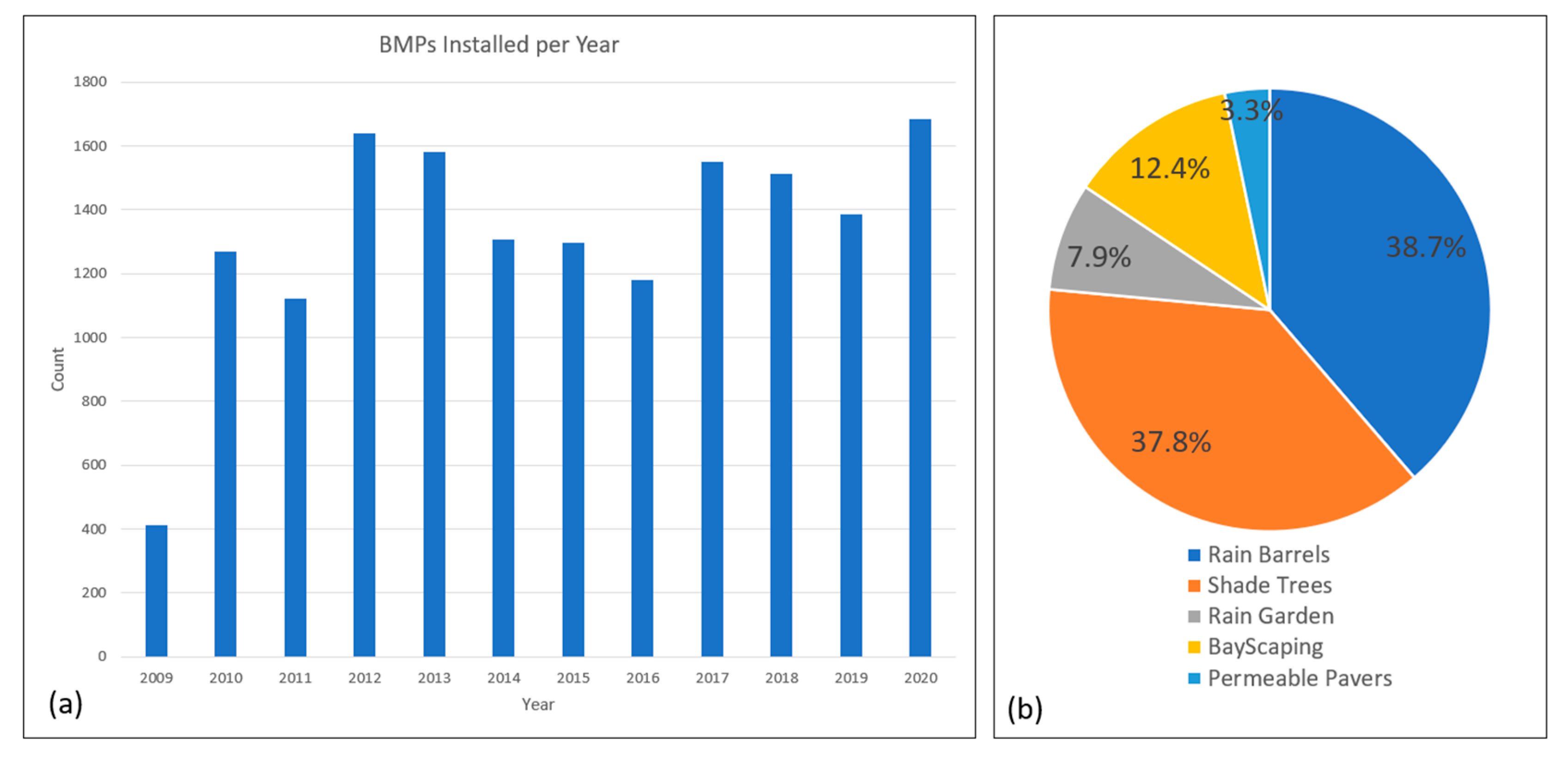
The RiverSmart Homes program started in 2009, and more than 15,000 BMPs have been installed across Washington, D.C., through this project. For each installation, the precise geographic location of the BMP, its type, and its date of implementation have been recorded in the publicly available RiverSmart Homes program database (Figure 1c). Most BMPs are found in residential areas of the northern and northeastern parts of Washington, D.C., where wealthier neighborhoods are located, and fewer BMPs are found in the southwestern and southeastern neighborhoods. The number of new BMPs installed each year, from the year 2009 to the year 2020, is shown in Figure 2. Approximately 400 BMPs were installed in the first year of the program (2009), and this substantially increased to 1200 new BMPs installed in the second year (2010), stabilizing at approximately 1400 new BMPs per year in the following ten years. The majority of BMPs installed under this program are rain barrels and shade trees, as shown in Figure 2b, which account for 39% and 38% of the BMP total, respectively. BayScaping is the third most popular BMP installed in this program (12% of participants). Rain gardens and permeable pavers are less popular, accounting for 8% and 3% of the installed total, respectively.

3.2. Physical and Demographic Factors for BMP Adoption Model

The socio-economic conditions of neighborhoods and the physical characteristics of landscapes have been proposed as major drivers for residential landowners and stakeholders in the decision to install BMPs [27,29,33,47,48,49]. Higher incomes and education levels are thought to foster adoption, while the percentage of rental properties in a neighborhood has the opposite effect. BMPs might also be found more frequently in neighborhoods with more abundant tree cover, suggesting a presumably more environmentally friendly disposition of residents, than in those that are more intensely paved. The behavioral propensity to install a BMP is further thought to be affected by the number of existing BMPs in one’s neighborhood, occurring as a socially diffusive process whereby contact with BMPs or communications with neighbors with BMPs enhances one’s likelihood of installing such a control measure as well.
To consider these potential factors in the development of the BMP adoption model, the set of input features considered in this work initially included 4 physical features and 17 demographic features (Table 3). Most of these features were obtained from the 2010 U.S. Census and 2010 ACS 5-year survey. The mean, median, standard deviation, minimum, and maximum values of each feature are included in the table below based on the values obtained for the 179 census tracts in Washington, D.C.
The selected physical features were the total area, total residential area, percentage of canopy in residential area, and average distance to nearest BMPs. The total area is the size of the census tract and ranges from 0.17 to 11 k m 2 , with a median size of 0.6 k m 2 . The total residential area is the sum of the areas of residential parcels in each census tract and ranges from 0 to 1 k m 2 , which generally represents approximately 20% of the size of a tract. It should be noted that as this study concentrated on the adoption of BMPs by households in residential lots, and tracts where the residential area is zero were neglected in the model development and application processes here. The percentage of canopy in residential areas was calculated by dividing the total canopy area in residential parcel lots by the total area of residential parcels in each census tract, and the percentages ranged from 0 to 48%. The average distance to the nearest BMP is the average of the minimum distance between each residential parcel lot and the registered location of the nearest BMP in the RiverSmart Homes database, ranging from 0 to approximately 3 k m .
Seventeen demographic features related to population and household characteristics were also considered in the set of potential model inputs in this research. These features were separately computed for each tract and included the total population, total number of households, population density and household density per 1000 m 2 , percentage of different population groups, median household income, median age, poverty rate, vacant rate, rental rate, and education level. We also considered the average area per household, which is calculated as the total residential parcel size divided by the total number of households in each tract. It is expected that a subset of these 17 demographic features and of the 4 physical inputs have a larger effect on BMP adoption than the rest; therefore, a reduced model that uses this subset could be used in practical applications. The identification of such a subset will be pursued below once the best form of the model has been identified.
For the linear regression model, we employed a statistical t-test to determine the significance of each variable. This test provides a p-value for each variable, reflecting the probability that the variable’s actual effect is null (insignificant). By selecting only those variables with p-values that are less than 5%, we adhere to a common convention in statistical analysis: only accepting variables that have less than a 5% probability of having a null effect as significant (i.e., there is at least 95% probability that they have a significant effect). This technique aids in preventing the model from overfitting by incorporating irrelevant variables. For LASSO regression, ridge regression, support vector regression (SVR), and random forest regression, we included all available variables in the census tracts, as these techniques have built-in mechanisms for handling a large number of predictors.

3.3. Potential BMP Adoption Models and Evaluation Metrics

Five predictive models were selected in this study for their evaluation as potential predictors of yearly BMP adoption likelihood based off of the physical and demographic features of the census tracts: linear regression, LASSO regression, ridge regression, support vector regression, and random forest models [38,39,40,41]. The ordinary linear regression model is of the form shown in Equation (1), expressed here for a single year of prediction, for simplicity:
f i = β 0 + β 1 x i 1 + β 2 x i 2 +
where f i is the predicted BMP adoption likelihood in census tract i (output variable), expressed as the number of newly installed BMPs per 1000 households in this tract one year after conditions were as described in the model inputs on the right-hand side of the equation. The physical and demographic features of the tract, which are the model’s inputs, are represented by the variable x i j , where i is the tract number and j is the feature index. The parameters denoted by β j are the coefficients that weigh the importance of feature j in producing the model’s output and are determined by the common least-square-error (LSE) process applied between the 1969 target values obtained from the RiverSmart database, denoted as y i , and the 41,349 values of input features from the Census (i.e., 1969 × (17 + 4)). The LSE approach guarantees that this linear model has a bias of zero (i.e., zero mean error) but does not imply that the model accurately predicts BMP adoption. In particular, the model is limited by its linear form, and the interpretability of its parameters may be affected by a non-zero covariance between input variables.
The accuracy of the simple linear model and of the other candidates for BMP adoption prediction was evaluated using 3 commonly used metrics: the coefficient of determination (R2), the percentage of bias (PBIAS), and the mean-square-error (MSE). The mathematical forms of these metrics are presented in Equations (2)–(4):
R 2 = 1 i f i y i 2 i y i y ¯ 2
P B I A S = i f i y i i y i × 100
M S E = 1 n i f i y i 2
where f i and y i have the same meaning as used earlier and y ¯ is the mean value of y i . The coefficient of determination, R2 (also called the Nash–Sutcliffe efficiency coefficient, NSE), quantifies the amount of variance in the observed variable (y) that is explained by the model. A value of 1 (the maximum possible) indicates a perfect prediction. In linear regression, R2 is equal to the square of the coefficient of linear correlation, but this equivalence breaks down under nonlinear parameterization approaches. PBIAS measures the average tendency of the predicted values to be larger or smaller than observed ones (it is the ratio of the mean error to the mean observed value). A value of 0 indicates perfect predictions. MSE is the mean of squared errors between the model output and observations, with 0 indicating a perfect fit once again. In addition to these metrics, for the case of linear regression, a t-test was conducted to evaluate the significance of each of the model’s input variables, with an early view towards potential model simplification.
LASSO and ridge regressions use a linear predictive model that is of the same form as that shown in Equation (1) but they substitute nonlinear parameter estimation techniques to the linear LSE process [40]. As a result, the model coefficients, β j , are determined in ways that may increase R2 relative to that obtained by LSE but no longer guarantee zero bias (and this also breaks the equivalence between R2 and the square of the correlation coefficient). Both methods have found uses in machine learning as well as statistics. LASSO (least absolute shrinkage and selection operator) and ridge regression were developed to mitigate issues related to high degrees of covariance between model input variables, which may occur with the socio-economic variables that are in the present study. To this effect, LASSO regression adds an L1 regularization term ( λ | β i | ) into the ordinary regression system, while ridge regression adds an L2 regularization term ( λ | β i | 2 ) [39]. These terms can be viewed as penalty terms in the form of the resulting optimization problem and serve as the trade-off bias accuracy for determination (or efficiency). In this study, both LASSO and ridge regressions were applied for the prediction of BMP adoption likelihood using the same dataset as that used for the ordinary least squares, and both regressions were evaluated using the 3 metrics discussed above and were compared with the linear regression model.
The support vector and random forest modeling approaches are extensions of supervised classification methods in which the model’s outputs can be arbitrary numbers rather than just individual classes. These methods seek to partition the space of model input values into characteristic sub-spaces, wherein simple predictive sub-models can be applied within each sub-space. Support vector models perform this partitioning by using hyperplanes, as shown in Figure 3a; random forest models use binary classification (or decision) trees instead (Figure 3b). In support vector methods, various mathematical functions, such as linear and polynomial functions, can be used to transform the input data into hyper dimensions, where classification may be achieved with greater accuracy. The coordinates of hyperplanes are iteratively adjusted using gradient descent methods to minimize the model prediction error. In random forest methods, decision trees replace hyperplanes, and their structure starts with the tree’s root on the first selected input variable, then splits based on threshold comparisons until a leaf node is reached. A large number of trees (above 100) is constructed using the random sequences of input variables, and thresholds are adjusted to approach the desired model outputs in each tree. The mean output from all trees is then taken as the prediction of this random forest. In this study, support vector and random forest approaches were used to construct corresponding models of BMP adoption likelihood. The accuracy of these models was assessed using the same metrics as those used for the LASSO, ridge, and linear regression, with the goal of identifying the most appropriate model for this behavior.

4. Results and Discussion

4.1. Results of BMP Adoption Model Development

The results of the ordinary least squares linear regression modeling of BMP adoption likelihood when considering all variables are detailed in Table 4. The results of the ordinary least squares linear regression modeling that only selected variables with p < 0.05 are shown in Table 5. Columns 2 and 3 in both Table 4 and Table 5 are coefficient β i and the standard error of regression coefficients of each feature. Columns 4 and 5 present parameters related to the significance of the model coefficients, the t-value, and the corresponding p-value. The t-value is the t-statistic of the overall model, and the associated p-value represents the likelihood that the t-statistic occurs by chance if the null hypothesis of no relationship between the dependent variable and independent variable is true.
In this model, the correlation with BMP adoption rate is positive for canopy cover, residential population density, and average lot area per household, but negative for the other six input features. Increasing BMP adoption likelihood with canopy cover and lot size appears reasonable, as does a decreasing rate of adoption with increasing rental rates and population density (at tract-level), which is consist with former research [50]. The identified negative association between BMP adoption rate and distance to the nearest BMP further seems consistent with social diffusion theory, whereby individuals located closer to an installed BMP are more likely to also implement a BMP themselves in the upcoming year. Negative associations of BMP adoption rate with median household income may be due to the fact that higher-income households may have access to alternatives that achieve similar goals without the need for BMPs or that these households may have installed such BMPs before the program. Poverty rate, which still disproportionately affects African American populations in the area of Washington, D.C., and elsewhere in the U.S. more than other groups, could be a more likely explanation for low BMP adoption rates.
The performance metrics for all regression models of BMP adoption likelihood are presented in Table 6. All models were trained using 70% of the dataset and were tested on the other 30%. The testing values are shown here. Linear regression and linear regression with features (p < 0.05) are shown in the first and second rows. The coefficient of determination of the linear regression model and linear regression model with features, R2, are 0.51 and 0.52, respectively, which indicates that the model explains just over half (51% or 52%) of the observed variability in BMP adoption rates in the study area. LASSO and ridge regression approaches attempt to limit the negative impacts of correlated inputs by trading determination for bias. LASSO regression accordingly produced a model that has a slightly higher coefficient of determination than ordinary least squares (R2 = 0.52) but at the cost of a negative bias, where the adoption rates are generally underpredicted. Ridge regression performs more poorly by providing no improvement in the coefficient of determination and causing a more significant underprediction than the LASSO model. Neither approach can be considered better than the ordinary least squares model in this study.
The accuracy of the support vector and random forest models of BMP adoption likelihood are also presented in Table 6. These modeling approaches use different methods to extend the classification, resulting in globally nonlinear models with quite different behaviors. The support vector model is found to explain only 13% of the variability in observed BMP adoption rates (R2 = 0.13) and produces predictions with the most bias out of the tested methods. The random forest model, on the other hand, explains the largest amount of observed variability in adoption rates at 67%, although it also tends to underpredict adoption, which is listed here by an average of over 7%; this suggests that it predicts low BMP adoption rates better than larger ones wherein most of its underpredictions would be located. The accurate prediction of the lower adoption rates corresponds to the preferred behavior for this model, which is targeted at the identification of zones with low likelihoods of spontaneous BMP installation, where social interventions should be focused for maximum return on environmental investments.
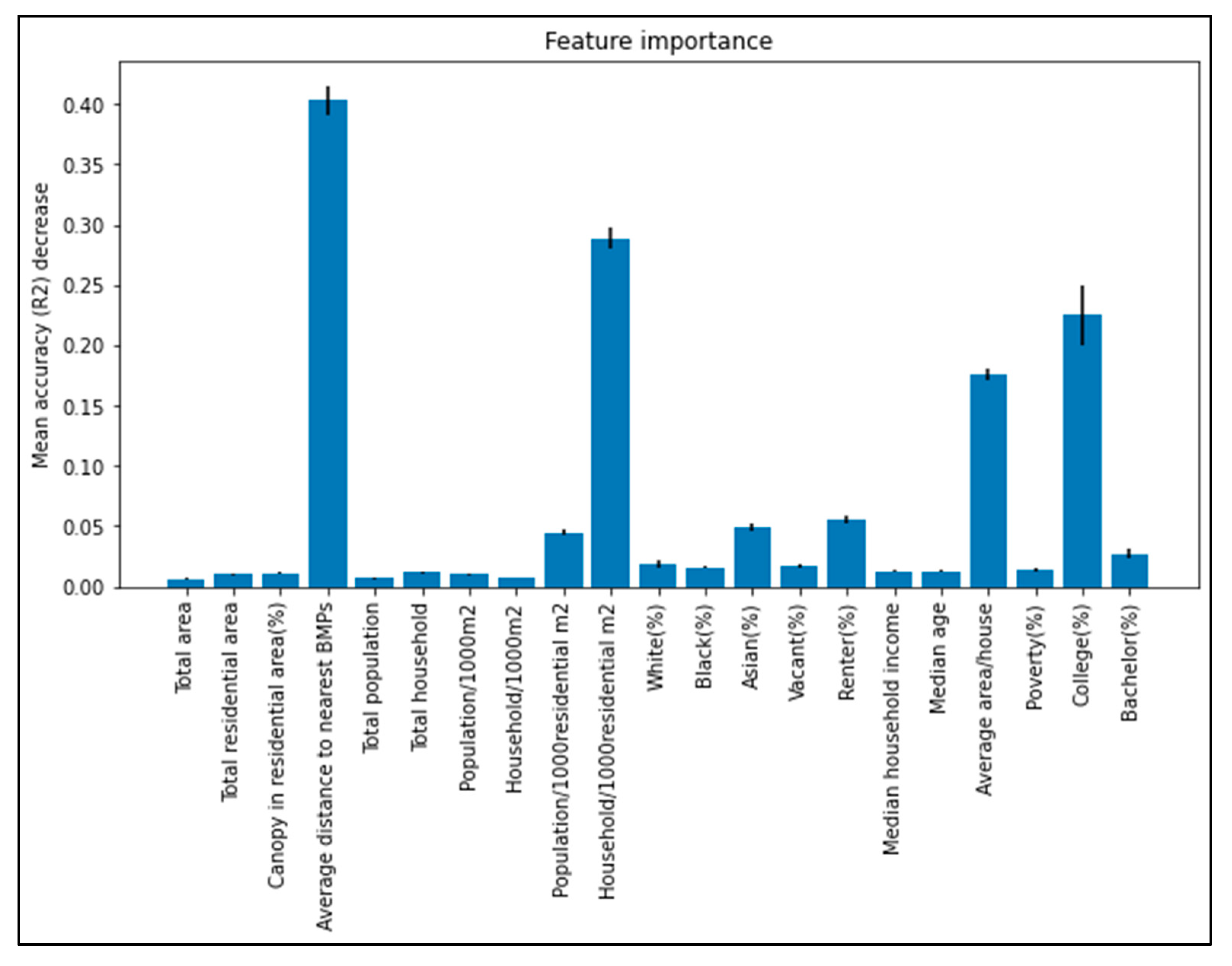
Based on the results of the performance evaluation of the six candidate BMP adoption likelihood models presented above, the random forest model was selected as the model of choice for this study. Accordingly, this model was subjected to a sensitivity analysis to determine the relative importance that each of its 21 input features had in producing its predictions. The sensitivity of a random forest model (or feature importance) is calculated by randomly shuffling each feature and computing the resulting change in its accuracy (R2) [51]. This process breaks the relationship between the selected feature and the model’s output, resulting in a drop in the value of R2 that reflects the degree to which the shuffled input impacts the accuracy of model predictions. The results of this process are presented in Figure 4 for each of the 21 model inputs and are expressed in terms of the reduction in R2 resulting from shuffling out that input. Four of the model’s inputs stand out as most significant from this analysis: (1) average distance to the nearest BMP; (2) residential housing density; (3) percentage of residents with a college degree; and (4) average area per house. If these features were entirely uncorrelated with each other, then removing just the first two from the model (i.e., average distance to the nearest BMP and residential housing density), would decrease its coefficient of determination down to essentially zero, indicating their substantial importance. The percentage of residents with a college degree is also very important, as shuffling it out reduces the model’s R2 value by 0.23 (from its original value of 0.67). Out of these four significant input features, two were also identified in the less accurate linear regression model: distance to BMPs and area per house. The less plausible features of the least squares model (median income and percentage of African American residents) are not identified as particularly significant in the more accurate random forest model. Conversely, the more plausible adoption factor of college education, which could reflect a better appreciation of environmental matters, is highlighted by this higher performing formulation.
Overall, the BMP adoption likelihood model developed in this study that was based on the random forest approach was found to show a better agreement to expected behavior than the other tested models. Its significant input features further suggest potential social intervention strategies aimed at increasing BMP adoption. For example, pilot BMP implementation projects could be started in areas of low spontaneous adoption to decrease the distance to the nearest BMP in these zones and jumpstart the social diffusion process of increasing BMP installation. Stormwater education campaigns could also be prioritized to zones with a lower percentage of college-educated residents to boost the environmental awareness of residents there and enhance their desire for BMP adoption.

4.2. Application of the BMP Adoption Likelihood Model

The application of the BMP adoption likelihood model was demonstrated on two watersheds with contrasting land cover and socio-economic conditions that are located in the region surrounding Washington, D.C. (Figure 1). The model predicted the yearly BMP adoption rates in the two watersheds and compared them on a whole watershed basis at the tract level over time. The model’s responses to changing the value of the initial density of BMPs in these watersheds and to changing socio-economic conditions were demonstrated. The NPS constituent control effectiveness that could be expected from spontaneous BMP adoption in each watershed, as predicted by the model and the need for targeted social interventions, were also evaluated and discussed. The description of these activities starts with that of the two study watersheds, which is followed by the algorithm used to apply the BMP adoption model spatio-temporally to these watersheds and by the outcomes of the resulting simulations.

4.2.1. BMP Adoption Simulation Algorithm

The BMP adoption likelihood model developed using the random forest approach mostly relies on census and land cover data for its inputs, which are readily transferable across study areas. However, one of its key input features, the distance to the nearest BMP, requires that specific spatial locations be selected for BMP installation within specific residential lots, which are contained within census tracts. An algorithm was developed to enable such selection, such that the predictions of BMP adoption rates can be applied over successive years by re-calculating the distances to the nearest BMPs, including those most recently implemented. This is an important component of the simulation process as it represents the effect of social diffusion on the temporal progression of BMP adoption by watershed residents. The developed simulation algorithm applies a random placement strategy to the positioning of new BMPs. In this approach, the number of new BMPs to install within a given tract is based on the random forest prediction of BMP adoption per 1000 households (multiplied by the number of households in the tract). These BMPs are randomly assigned to residential lots within the tract, with a probability that is calculated by following the binomial distribution, in inverse proportion to the distance between each lot and the nearest BMP. The resulting algorithm for BMP allocation proceeds along the following steps:
Step 1
Based on the initial BMP density setting (e.g., 1 per 1000 housing units), randomly selected N residential parcels for BMP allocation. Set step t = 0 .
Step 2
Calculate the distance of all residential lots to the nearest BMPs. Update the average minimum distance to BMPs for all census tracts.
Step 3
Predict the number n i new BMP adoption for census tract i based on the regression model.
Step 4
Randomly select n i residential parcels in census tract i for BMP adoption based on possibility p as detailed below:
4.1.
For each residential lot, find the maximum distance to the nearest BMP and use the maximum value minus the current distance to the nearest BMP for each residential lot as the weight.
4.2.
Calculate the allocation probability for each residential parcel as weight/sum_of_all_weights
Step 5
If the stop criterion is satisfied, terminate the process; else, set t = t + 1 , and go to Step 2.
This BMP adoption simulation was run for both watersheds in different settings. First, a basic ten-year simulation was run for the Watts Branch watershed and Watershed 263 using socio-economic data from the 2010 Census and an initial density of 1 BMP per 1000 households to establish baseline BMP adoption dynamics in both watersheds. Second, the socio-economic input features of the model were updated to those of the 2020 Census, and a new ten-year simulation was performed to evaluate the impact of these real-world changes on BMP adoption. The initial spatial density of BMPs was then changed to assess how that initial condition affected BMP adoption dynamics over a ten-year period. Lastly, adoption simulations were run for a long enough period to achieve the NPS pollution control target of having BMPs be implemented in 20% of the area of each watershed, and the time needed to achieve this coverage was compared between the two watersheds, as well as the eventual position of the BMPs, relative to that of the NPS constituent hotspots.

4.2.2. Baseline Simulation Results for BMP Adoption

Figure 5 presents the results of baseline BMP adoption simulations aggregated over the set of census tracts in each of the two study watersheds, with 1 BMP per 1000 households being the initial condition. In Watts Branch, the predicted BMP adoption rate is observed to increase relatively quickly during the first 4 years of the simulation, stabilizing at approximately 15 new BMPs per 1000 households per year. In contrast, Watershed 263’s BMP adoption rate initially increases somewhat quickly but more slowly than in Watts Branch and only for 2 years, after which it nearly stabilizes at approximately 5 new BMPs per 1000 households per year. Even though the initial BMP density is the same in the two watersheds, the overall BMP adoption rate in Watts Branch is much higher than in Watershed 263. We also note that an initial increase in BMP adoption rate followed by a stabilization of this rate, as predicted here by the adoption model for both watersheds, agrees with the adoption rate behavior observed for Washington, D.C., from the RiverSmart Homes data (Figure 2).
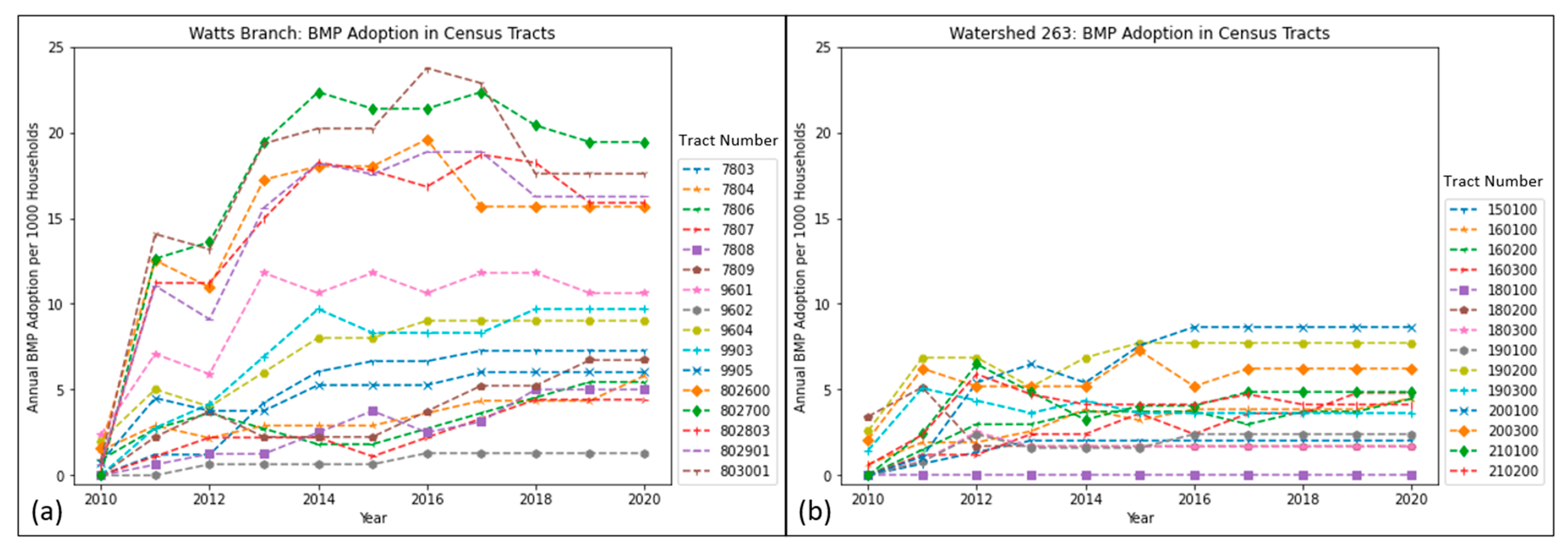
The details of the BMP adoption rates at the census tract level in both watersheds are shown in Figure 6. All census tracts show an increasing trend in the first several years, where the BMP adoption rates then remain unchanged for the following years; and the overall BMP adoption rates in most census tracts in Watts Branch are more significant than that in Watershed 263. In Watts Branch, initial BMP adoption densities are between zero and two in all tracts; then, they most sharply increase in the second year, reach the peak rate in about five years, and then fluctuate in the following five years. The census tracts of Watts Branch in the Maryland part (802,600–803,001) have higher BMP adoption rates than those in Washington, D.C. (7803–9905). A comparison of the socio-economic features between the census tracts in Maryland and in Washington, D.C., indicates better conditions in Maryland than in D.C. For example, the average number of housing units per 1000 residential square meters is close to 5 in Washington, D.C., but is only 2 in Maryland. The average canopy percentage (34% vs. 48%), median household income (USD 28,563 vs. USD 56,123), average area per housing unit (246 m2 vs. 556 m2), and poverty rate (29% vs. 13%) also favor Maryland above DC. Even though these tracts are in the same watershed, those located in Maryland correspond to “healthier” socio-economic conditions and have higher BMP adoption rates than those located in Washington, D.C. In contrast, all of the census tracts located in Watershed 263 have similar BMP adoption rates in the ten-year simulation results. Most tract-level BMP adoption rates increase in the first two or three years and then remain stable for the following seven years. The peak BMP adoption rate is between 3 and 10, with an average of 5 new BMPs per 1000 housing units per year. Compared with the census tracts in Watts Branch in Washington, D.C., about half of the census tracts in Watts Branch have a similar BMP adoption rate to that of Watershed 263. Overall, the BMP adoption rate is higher in Watts Branch than in Watershed 263, and this better performance results from the five “healthier” census tracts that are located in Maryland in this watershed.
Spatio-temporal maps of BMP adoption in Watts Branch and Watershed 263 are presented in Figure 7. Gray areas in this figure represent residential lots, green lines are the watershed boundaries, and red dots depict the predicted BMPs installed in those watersheds. The initial BMPs were randomly assigned to residential parcels at a density of 1 BMP per 1000 residential lots. Then, new BMPs were iteratively added to randomly selected parcels using the simulation algorithm; the results of that process are shown in the figure with a three-year time step. The results indicate that BMPs tend to be allocated in clusters, possibly as a result of social diffusion. For example, in Watts Branch, new BMPs accumulated higher density in tracts 802,600, 802,700, 802,901, and 803,001 in Maryland and 7809, 9604, and 9903 in Washington, D.C. This clustering also happens in Watershed 263. Census tracts such as 190,200, 190,300, 200,100, and 200,300 in the southern part of the watershed have a higher BMP density than tracts in the northern regions. The total predicted BMPs implemented in Watts Branch and Watershed 263 are 1727 (about 95 BMPs per km2) and 521 (about 70 BMPs per km2), respectively, for the duration of nine years. This difference in the level of implementation appropriately corresponds with differences in factors affecting BMP adoption rate in the two watersheds, such as median household income and poverty rate, all of which motivate the BMP adoption.

4.2.3. BMP Adoption Response to Changing Conditions

The impact of different BMP initial densities is shown in Figure 8. The initial BMP density changes from 0.5 per 1000 households to 1 per 1000 households, 2 per 1000 households, and 4 per 1000 households. The BMP adoption rates increased to a saturated platform after rising in the first several years. In the Watts Branch watershed, the BMP adoption rate increases to around eight in the second year and arrives at a peak rate of fourteen in five years. As for Watershed 263, lower initial BMP densities, such as 0.5 per 1000 households, need about three years to reach the top BMP adoption rate. In contrast, a higher initial BMP density of 2 per 1000 or 4 per 1000 needs only one year to achieve the peak BMP adoption rate. Therefore, BMP density will affect BMP adoption in the first several years, but this impact decreases as more and more BMP are implemented in the watersheds.
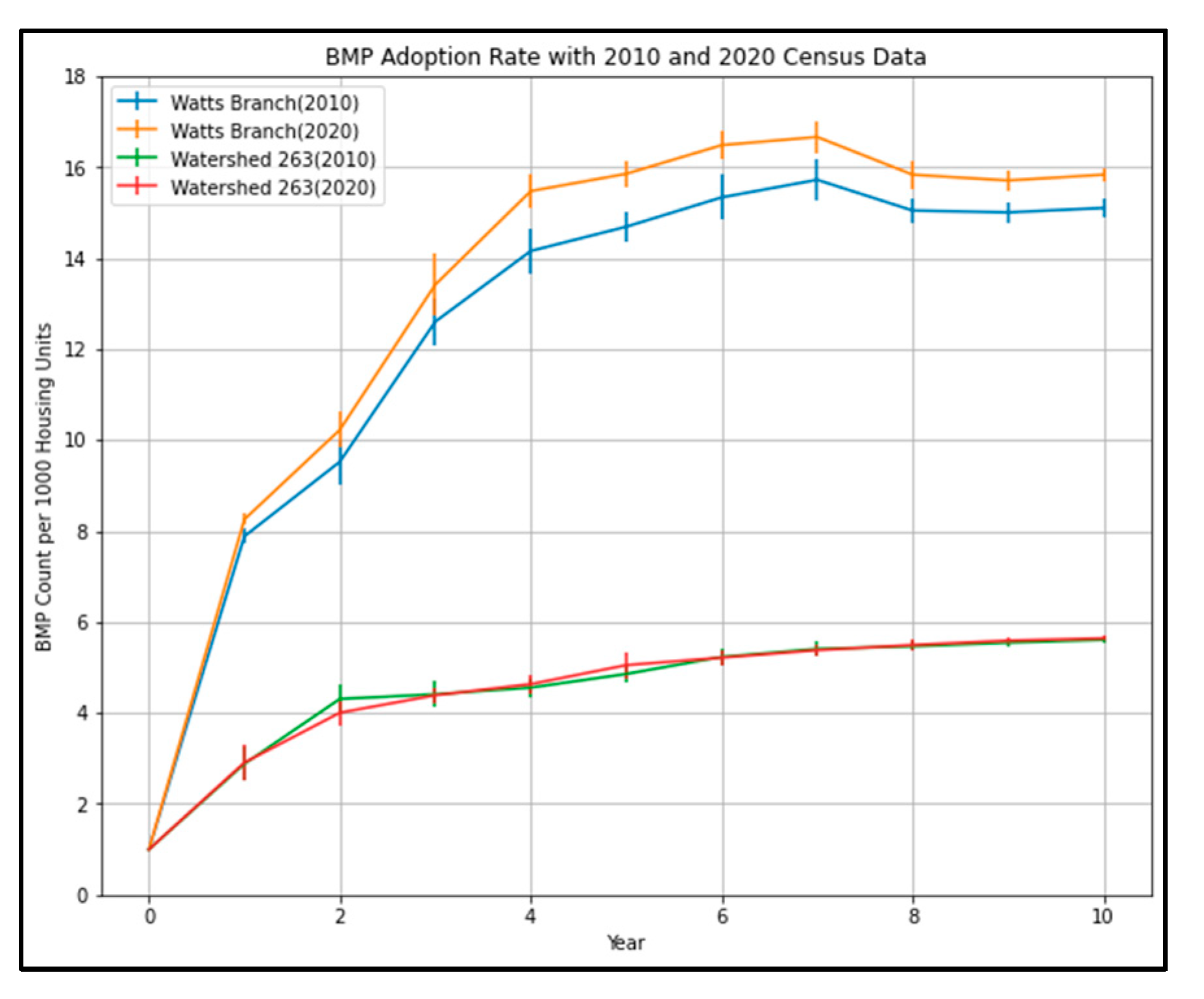
Figure 9 compares the BMP adoption rates with 2010 and 2020 census data in two watersheds. With the same initial BMP density, the BMP adoption rate in the Watts Branch watershed increased by about 10% when using the 2020 census data, whereas Watershed 263’s BMP adoption rate remains unchanged. Compared with the socio-economic data in these two watersheds (Table 1), many features in the Watts Branch watershed improved in ten years. For example, the total population in Watts Branch increased from 48,168 to 55,002, whereas the number in Watershed 263 decreased from 30,344 to 27,594. The poverty rate dropped from 24.29% to 21.21% in Watts Branch but increased from 35.45% to 39.24% in Watershed 263. We can also find some improvement in both watersheds, such as in median household income, vacant rate, and renter rate. This could explain why the peak BMP adoption rate in Watershed 263 remains unchanged in these two different year conditions.

4.2.4. BMP Adoption and NPS Constituent Control

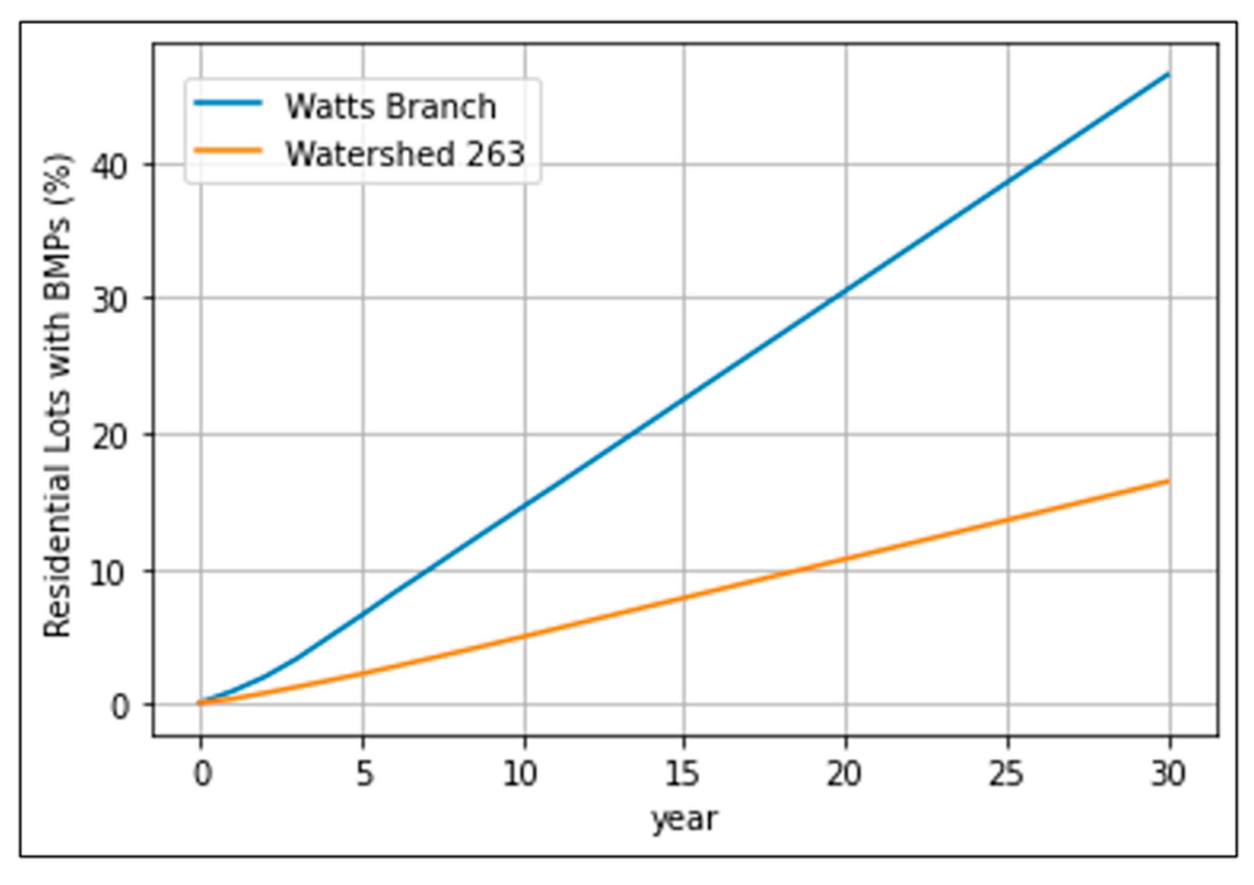
The percentage of residential lots covered by BMPs in 30 years is shown in Figure 10. In ten years, about 15% of the residential lots in Watts Branch will be covered by BMPs, but this number is only 6% in Watershed 263. If the simulation period extends to 30 years, then 48% of residential lots in Watts Branch will be covered by BMPs, but only 18% will be in Watershed 263. The BMP peak adoption rate is much higher in Watts Branch than in Watershed 263.
Based on our former research, 20% of the hotspot area in Watts Branch can account for 40–50% of the sediment, nitrogen, and phosphorus output and about 50% of the sediment and phosphorus in Watershed 263. Thus, if we choose 20% of the area as the BMP allocation goal, 14 years are needed in the Watts Branch watershed and more than 30 years are needed in Watershed 263 (37 years in simulation). As such, more social interventions should be required to have enough BMPs allocated in hotspot areas for NPS pollution control in Watershed 263.
To compare the BMP allocation with the nutrient’s (N and P) hotspots, we simulated the model in Watts Branch and Watershed 263 for 20 years. BMPs covered 20% of the residential lots in Watts Branch by year 14 (Figure 11a) but only 7.6% in Watershed 263 (Figure 11d). A SWAT model was used to simulate both watersheds, and the N and P hotspots (20% and 50% of the total output of N and P) are shown in Figure 11b,c,e,f. Looking at Watts Branch, most of Maryland’s N and P hotspots are covered by BMPs. Most of these are in residential areas, so the BMP allocation scenario in 14 years can potentially treat the NPS pollutants (N and P) effectively.
In contrast, a significant portion of nutrient hotspots in the southwest of Watershed 263 is open space, and BMPs neglect these nitrogen hotspots. Moreover, the northern part of the watershed is also open space, where the BMPs also ignore nitrogen and phosphorus hotspots. Thus, 14 years of simulation have not tackled the nutrients properly. In summary, to effectively control the NPS pollutants in watershed 263, social intervention is needed to increase the BMP adoption speed. Moreover, as some NPS pollutants hotspots are not in residential areas, BMPs that are implemented by local stakeholders as opposed to residents are necessary to treat the NPS pollution.

5. Conclusions

This research developed regression BMP adoption models based on the actual physical and demographic features data from Washington, D.C. The best-performing model is the random forest regression, with its R2 value of 0.67, PBIAS of −7.24, and MSE of 19.11. Based on this model, the spatio-temporal dynamics of BMP adoption behavior in two urban watersheds, Watts Branch (relatively “healthy”) and Watershed 263 (relatively “unhealthy”), were quantitatively analyzed. This research shows that distance to the nearest BMPs, education level, residential property (size, canopy value), and economic factors significantly impact BMP adoption. This simulation of BMP adoption in two watersheds also conforms to our estimation of “healthy” (Watts Branch) and “unhealthy” (Watershed 263) watersheds, where the BMP adoption rate in Watts Branch is much higher than that of Watershed 263. Even in the same watershed, “healthy” census tracts will have a much higher BMP adoption rate than “unhealthy” census tracts. Compared with the BMP adoption scenarios, to achieve 20% of residential parcels being covered by BMPs, Watts Branch will need 14 years; Watershed 263 will need more than 30 years. However, this three-fold longer time could not ensure the NPS pollutants control goal. A significant portion of the NPS pollutants hotspots are in open space, and other stakeholders aside from residents are needed to implement the BMPs.
The adoption of BMPs is influenced by a range of factors. These include the percentage of canopy coverage, average distance to the nearest BMPs, population density in residential areas, and average area per household, all of which have been found to have positive correlations with BMP adoption. In contrast, certain factors are observed to negatively impact BMP adoption. These include a high renter rate and a higher percentage of underrepresented population in the area. These factors can potentially represent socio-economic barriers to BMP adoption. Given these insights, it is imperative to design social interventions aimed at mitigating these negative impacts. Such interventions could focus on improving awareness about the benefits of BMPs, providing resources for the implementation or advocation of policy changes that encourage BMP adoption in all community sectors, thereby making environmental sustainability more accessible and equitable.
In order to counter factors that negatively affect BMP adoption, such as high renter rates and socio-economic disparities, a targeted approach is essential. For instance, educational programs can be designed to inform and engage renters about the benefits of BMPs, which could lead to increased uptake, even among this transient population. Efforts should also be made to increase BMP adoption within underrepresented communities. This could involve outreach programs to raise awareness about BMPs and their environmental and health benefits or by partnering with community leaders to drive adoption. Subsidies or other financial incentives could be introduced to make BMP implementation more feasible for households in these communities. In areas where BMP adoption is lower due to population density or lack of canopy coverage, green initiatives can be promoted.
Overall, this research quantitatively demonstrates the spatio-temporal patterns of BMP adoption in urban areas. This research confirms that a “healthy” watershed will treat NPS pollutants effectively and emphasizes the importance of social intervention in the “unhealthy” watershed or census tracts. More work is needed in the pollutant hotspots to promote BMP adoption and achieve NPS control goals. Beyond the scope of residential areas, the cleanup and transformation of non-residential zones such as industrial regions, which are termed “brown-field development”, offers significant potential benefits. However, this research did not include an assessment of the “brown-field” areas within the study’s watersheds. Future research should explore the economic incentives and environmental remediation possibilities that are associated with such initiatives.

Author Contributions

Conceptualization, Z.Z., H.M., A.K.R. and A.S.; methodology, Z.Z. and H.M.; software, Z.Z.; validation, Z.Z., H.M., and A.S.; formal analysis, Z.Z.; investigation, Z.Z. and A.K.R.; resources, H.M., A.S. and P.T.L.; writing—original draft preparation, Z.Z. and H.M.; writing review and editing, H.M., A.S., A.K.R. and P.T.L.; visualization, Z.Z.; supervision, H.M. and A.S.; project administration, P.T.L.; funding acquisition, H.M, A.S., A.K.R. and P.T.L. All authors have read and agreed to the published version of the manuscript.

Funding

This research was funded by the National Science Foundation under grant number NSF-ICER # 1824807.

Data Availability Statement

Not applicable.

Conflicts of Interest

The authors declare no conflict of interest.

References

  1. USEPA. National Water Quality Inventory: Report to Congress; US Environmental Protection Agency, Office of Water: Washington, DC, USA, 2017.
  2. USEPA. Nonpoint-Source Pollution: The Nation’s Largest Water Quality Problem; US Environmental Protection Agency, Office of Water: Washington, DC, USA, 1996.
  3. Brown, T.C.; Froemke, P. Nationwide assessment of nonpoint source threats to water quality. BioScience 2012, 62, 136–146. [Google Scholar] [CrossRef] [Green Version]
  4. Deb, K.; Agrawal, S.; Pratap, A.; Meyarivan, T. A fast elitist non-dominated sorting genetic algorithm for multi-objective optimization: NSGA-II. In Proceedings of the International Conference on Parallel Problem Solving from Nature, Paris, France, 18–20 September 2000; pp. 849–858. [Google Scholar]
  5. Dzikiewicz, M. Activities in nonpoint pollution control in rural areas of Poland. Ecol. Eng. 2000, 14, 429–434. [Google Scholar] [CrossRef]
  6. Hardy, S.D.; Koontz, T.M. Reducing nonpoint source pollution through collaboration: Policies and programs across the US States. Environ. Manag. 2008, 41, 301–310. [Google Scholar] [CrossRef] [PubMed]
  7. Lian, Q.; Yao, L.; Uddin Ahmad, Z.; Lei, X.; Islam, F.; Zappi, M.E.; Gang, D.D. Nonpoint source pollution. Water Environ. Res. 2019, 91, 1114–1128. [Google Scholar] [CrossRef] [Green Version]
  8. Baker, L.A. Introduction to nonpoint source pollution in the United States and prospects for wetland use. Ecol. Eng. 1992, 1, 1–26. [Google Scholar] [CrossRef]
  9. McCoy, N.; Chao, B.; Gang, D.D. Nonpoint source pollution. Water Environ. Res. 2015, 87, 1576–1594. [Google Scholar] [CrossRef]
  10. Xepapadeas, A. The economics of non-point-source pollution. Annu. Rev. Resour. Econ. 2011, 3, 355–373. [Google Scholar] [CrossRef] [Green Version]
  11. Xiang, C.; Wang, Y.; Liu, H. A scientometrics review on nonpoint source pollution research. Ecol. Eng. 2017, 99, 400–408. [Google Scholar] [CrossRef]
  12. Guo, T.; Srivastava, A.; Flanagan, D.C.; Liu, Y.; Engel, B.A.; McIntosh, M.M. Evaluation of Costs and Efficiencies of Urban Low Impact Development (LID) Practices on Stormwater Runoff and Soil Erosion in an Urban Watershed Using the Water Erosion Prediction Project (WEPP) Model. Water 2021, 13, 2076. [Google Scholar] [CrossRef]
  13. Hsu, D.; Lim, T.C.; Meng, T. Rocky steps towards adaptive management and adaptive governance in implementing green infrastructure at urban scale in Philadelphia. Urban For. Urban Green. 2020, 55, 126791. [Google Scholar] [CrossRef]
  14. Ice, G. History of innovative best management practice development and its role in addressing water quality limited waterbodies. J. Environ. Eng. 2004, 130, 684–689. [Google Scholar] [CrossRef]
  15. Zhang, K.; Chui, T.F.M. A comprehensive review of spatial allocation of LID-BMP-GI practices: Strategies and optimization tools. Sci. Total Environ. 2018, 621, 915–929. [Google Scholar] [CrossRef] [PubMed]
  16. Martin, P. Sustainable Urban Drainage Systems: Design Manual for England and Wales; Ciria: Soria, Spain, 2000. [Google Scholar]
  17. Fletcher, T.D.; Shuster, W.; Hunt, W.F.; Ashley, R.; Butler, D.; Arthur, S.; Trowsdale, S.; Barraud, S.; Semadeni-Davies, A.; Bertrand-Krajewski, J.-L. SUDS, LID, BMPs, WSUD and more–The evolution and application of terminology surrounding urban drainage. Urban Water J. 2015, 12, 525–542. [Google Scholar] [CrossRef]
  18. Council, N.R. Urban Stormwater Management in the United States; National Academies Press: Washington, DC, USA, 2009. [Google Scholar]
  19. Dietz, M.E.; Clausen, J.C. A field evaluation of rain garden flow and pollutant treatment. Water Air Soil Pollut. 2005, 167, 123–138. [Google Scholar] [CrossRef]
  20. Ahiablame, L.M.; Engel, B.A.; Chaubey, I. Effectiveness of low impact development practices: Literature review and suggestions for future research. Water Air Soil Pollut. 2012, 223, 4253–4273. [Google Scholar] [CrossRef]
  21. Ahiablame, L.M.; Engel, B.A.; Chaubey, I. Effectiveness of low impact development practices in two urbanized watersheds: Retrofitting with rain barrel/cistern and porous pavement. J. Environ. Manag. 2013, 119, 151–161. [Google Scholar] [CrossRef]
  22. Benedict, M.A.; McMahon, E.T. Green Infrastructure: Linking Landscapes and Communities; Island Press: Washington, DC, USA, 2006. [Google Scholar]
  23. Coutts, C.; Hahn, M. Green infrastructure, ecosystem services, and human health. Int. J. Environ. Res. Public Health 2015, 12, 9768–9798. [Google Scholar] [CrossRef] [Green Version]
  24. López-Ballesteros, A.; Senent-Aparicio, J.; Srinivasan, R.; Pérez-Sánchez, J. Assessing the Impact of Best Management Practices in a Highly Anthropogenic and Ungauged Watershed Using the SWAT Model: A Case Study in the El Beal Watershed (Southeast Spain). Agronomy 2019, 9, 576. [Google Scholar] [CrossRef] [Green Version]
  25. Mao, X.; Jia, H.; Shaw, L.Y. Assessing the ecological benefits of aggregate LID-BMPs through modelling. Ecol. Model. 2017, 353, 139–149. [Google Scholar] [CrossRef]
  26. Shafique, M.; Kim, R.; Rafiq, M. Green roof benefits, opportunities and challenges—A review. Renew. Sustain. Energy Rev. 2018, 90, 757–773. [Google Scholar] [CrossRef]
  27. Tayouga, S.J.; Gagné, S.A. The socio-ecological factors that influence the adoption of green infrastructure. Sustainability 2016, 8, 1277. [Google Scholar] [CrossRef] [Green Version]
  28. Barnhill, K.; Smardon, R. Gaining ground: Green infrastructure attitudes and perceptions from stakeholders in Syracuse, New York. Environ. Pract. 2012, 14, 6–16. [Google Scholar] [CrossRef]
  29. Brehm, J.M.; Pasko, D.K.; Eisenhauer, B.W. Identifying key factors in homeowner’s adoption of water quality best management practices. Env. Manag. 2013, 52, 113–122. [Google Scholar] [CrossRef] [PubMed]
  30. Lim, T.C. An empirical study of spatial-temporal growth patterns of a voluntary residential green infrastructure program. J. Environ. Plan. Manag. 2018, 61, 1363–1382. [Google Scholar] [CrossRef]
  31. Lim, T.C. Revitalizing Urban Neighborhoods by Adopting Green Infrastructure: The Case of Washington DC; Virginia Tech: Blacksburg, VA, USA, 2018. [Google Scholar]
  32. Patra, D.; Chanse, V.; Rockler, A.; Wilson, S.; Montas, H.; Shirmohammadi, A.; Leisnham, P.T. Towards attaining green sustainability goals of cities through social transitions: Comparing stakeholders’ knowledge and perceptions between two Chesapeake Bay watersheds, USA. Sustain. Cities Soc. 2021, 75, 103318. [Google Scholar] [CrossRef]
  33. Maeda, P.K.; Chanse, V.; Rockler, H.; Montas, H.; Shirmohammadi, A.; Wilson, S.; Leisnham, P.T. Linking stormwater best management practices to social factors in two suburban watersheds. PLoS ONE 2018, 13, e0202638. [Google Scholar] [CrossRef] [Green Version]
  34. Chanse, V.; Mohammed, A.; Wilson, S.; Delamarre, L.; Rockler, A.; Leisnham, P.T.; Shirmohammadi, A.; Montas, H. New approaches to facilitate learning from youth: Exploring the use of Photovoice in identifying local watershed issues. J. Environ. Educ. 2017, 48, 109–120. [Google Scholar] [CrossRef]
  35. Smith, L.K.M.; Lynes, J.K.; Wolfe, S.E. Community-based social marketing-creating lasting, sustainable, environmental change: Case study of a household stormwater managment program in the resgion of Waterloo, Ontario. Soc. Mark. Q. 2019, 25, 308–326. [Google Scholar] [CrossRef]
  36. Hazbavi, Z.; Sadeghi, S.H.; Gholamalifard, M.; Davudirad, A.A. Watershed health assessment using the pressure–state–response (PSR) framework. Land Degrad. Dev. 2020, 31, 3–19. [Google Scholar] [CrossRef]
  37. Hazbavi, Z.; Sadeghi, S.H.R. Watershed health characterization using reliability–resilience–vulnerability conceptual framework based on hydrological responses. Land Degrad. Dev. 2017, 28, 1528–1537. [Google Scholar] [CrossRef]
  38. Awad, M.; Khanna, R. Support vector regression. In Efficient Learning Machines; Springer: Berlin/Heidelberg, Germany, 2015; pp. 67–80. [Google Scholar]
  39. McDonald, G.C. Ridge regression. Wiley Interdiscip. Rev. Comput. Stat. 2009, 1, 93–100. [Google Scholar] [CrossRef]
  40. Ranstam, J.; Cook, J. LASSO regression. J. Br. Surg. 2018, 105, 1348. [Google Scholar] [CrossRef]
  41. Segal, M.R. Machine Learning Benchmarks and Random Forest Regression; eScholarship: Oakland, CA, USA, 2004. [Google Scholar]
  42. Leets, L.; Sprenger, A.; Hartman, R.O.; Jackson, J.H.; Britt, M.; Gulley, A.; Thomas, J.S.; Wijesinghe, S. Promoting tree equity in Washington, DC. Trees For. People 2022, 7, 100209. [Google Scholar] [CrossRef]
  43. Department of Energy and Environment. RiverSmart Homes. 2021. Available online: https://doee.dc.gov/service/riversmart-homes (accessed on 1 May 2022).
  44. Wang, Y.; Montas, H.; Leisnham, P.T.; Brubaker, K.; Shirmohammadi, A.; Chanse, V.; Rockler, A. A diagnostic decision support system for BMP selection in a small urban watershed. Water Resour. Manag. 2017, 31, 1649–1664. [Google Scholar] [CrossRef]
  45. Wilfong, M.; Patra, D.; Pavao-Zuckerman, M.; Leisnham, P.T. Diffusing responsibility, decentralizing infrastructure: Hydrosocial relationships within the shifting stormwater management paradigm. J. Environ. Plan. Manag. 2022, 1–22. [Google Scholar] [CrossRef]
  46. Wilfong, M.; Paolisso, M.; Patra, D.; Pavao-Zuckerman, M.; Leisnham, P.T. Shifting paradigms in stormwater management–hydrosocial relations and stormwater hydrocitizenship. J. Environ. Policy Plan. 2023, 25, 429–442. [Google Scholar] [CrossRef]
  47. Baptiste, A.K.; Foley, C.; Smardon, R. Understanding urban neighborhood differences in willingness to implement green infrastructure measures: A case study of Syracuse, NY. Landsc. Urban Plan. 2015, 136, 1–12. [Google Scholar] [CrossRef]
  48. Brown, H.L.; Bos, D.G.; Walsh, C.J.; Fletcher, T.D.; RossRakesh, S. More than money: How multiple factors influence householder participation in at-source stormwater management. J. Environ. Plan. Manag. 2016, 59, 79–97. [Google Scholar] [CrossRef]
  49. McPhillips, L.E.; Matsler, A.M. Temporal evolution of green stormwater infrastructure strategies in three US cities. Front. Built Environ. 2018, 4, 26. [Google Scholar] [CrossRef] [Green Version]
  50. Ando, A.W.; Freitas, L.P. Consumer demand for green stormwater management technology in an urban setting: The case of Chicago rain barrels. Water Resour. Res. 2011, 47, 12. [Google Scholar] [CrossRef]
  51. Grömping, U. Variable importance assessment in regression: Linear regression versus random forest. Am. Stat. 2009, 63, 308–319. [Google Scholar] [CrossRef]
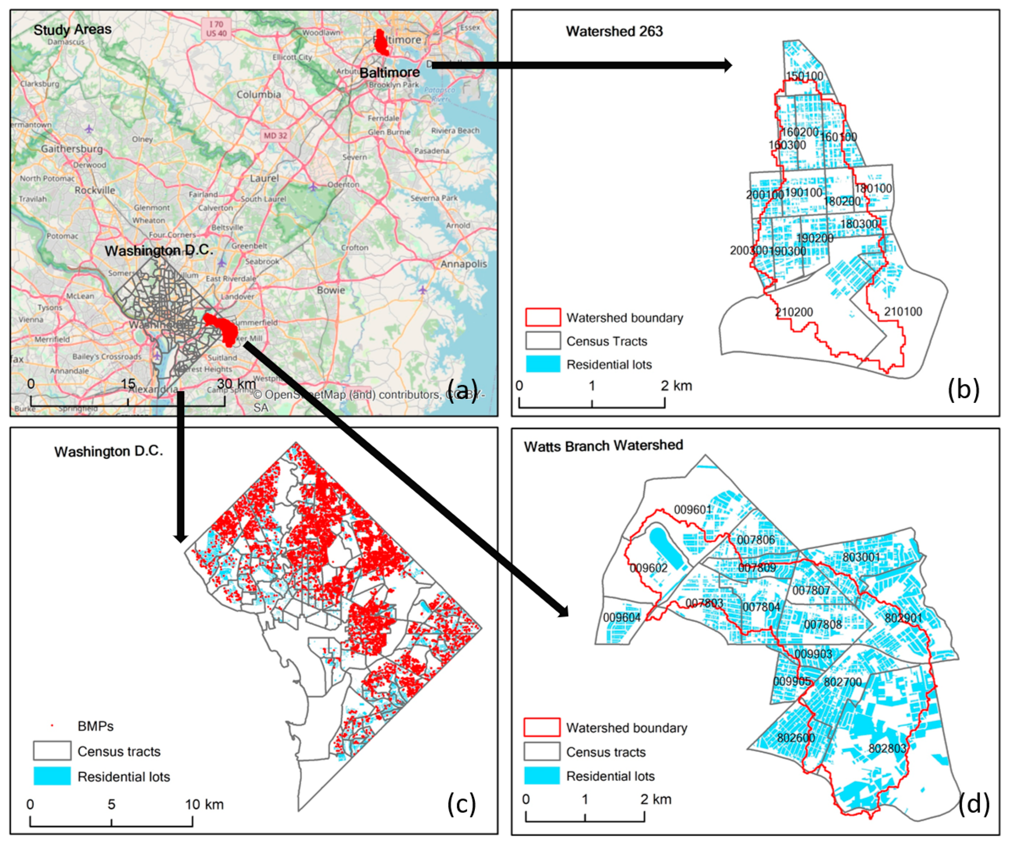
Figure 1. Study area and locations. (a) Relative location of the Washington, D.C., Watts Branch watershed and Watershed 263; (b) census tracts and residential lots in Watershed 263; (c) total BMPs installed between 2009 and 2020 in Washington, D.C.; (d) census tracts and residential lots in Watts Branch.
Water 15 02549 g001
Figure 2. BMPs installed through the RiverSmart Home project in Washington, D.C.; (a) BMPs installed each year; (b) Percentages of the different types of all BMPs installed between 2009 and 2020.
Water 15 02549 g002
Figure 3. Illustration of a hyperplane used in support vector regression; (a) decision trees used in random forest regression (b).
Water 15 02549 g003
Figure 4. Feature importance of the random forest regression model of BMP adoption likelihood identified using the input feature permutation approach.
Water 15 02549 g004
Figure 5. BMP adoption in two watersheds in a ten-year simulation.
Water 15 02549 g005
Figure 6. Annual BMP adoption rate in each census in Watts Branch (a) and Watershed 263 (b).
Water 15 02549 g006
Figure 7. Spatio-temporal BMP adoption in both watersheds in a three-year step. Red dots: predicted BMPs adoption, gray areas: residential lots; green lines: watershed boundary; (ad) BMPs adoption in a 3-year step around Watts Branch Watershed, (eh) BMPs adoption in a 3-year step around watershed 263.
Water 15 02549 g007
Figure 8. Impacts of initial BMP density on BMP adoption in (a) Watts Branch Watershed and (b) Watershed 263.
Water 15 02549 g008
Figure 9. BMP adoption rates simulated by the random forest model for ten years using 2010 and 2020 census tract data for Watts Branch and Watershed 263.
Water 15 02549 g009
Figure 10. Percentage of the residential lot covered by BMPs in 30 years.
Water 15 02549 g010
Figure 11. BMP allocation and nutrient hotspots in two watersheds. (a) Map depicting 20% of residential lots covered by BMPs in Watts Branch in 14 years; (b,c) map depicting nitrogen and phosphorus output hotpots in Watts Branch, as calculated by SWAT simulation; (d) map depicting 7.6% of residential lots covered by BMPs in Watershed 263; (e,f) map depicting nitrogen and phosphorus output hotpots in Watershed 263, as calculated by SWAT simulation.
Water 15 02549 g011
Table 1. Major features of the Watts Branch watershed and Watershed 263 in 2010 and 2020.
Watts BranchWatershed 263
2010202020102020
Physical
Total area (km2)18.817.43
Residential area (km2)6.911.33
Total residential lots13,32711,863
Demographic
Total population48,16855,00230,34427,594
Total housing units20,53622,02116,66817,054
Vacant rate (%)11103033
Renter rate (%)51476769
Poverty rate (%)24213539
College (%)22271622
Bachelor’s degree (%)81399
Median household incomeUSD 37,176USD 52,798USD 27,125USD 32,362
Table 2. BMP and copayment details.
FeaturesCopaymentTotal Costs
Rain barrelsUSD 50 or USD 70 per rain barrel, depending on the types (limit two)USD 150 per rain barrel
Shade treesUSD 0 per shade tree (no limit)USD 50 per shade tree
Rain gardensUSD 100 per 50 sq. ft. (USD 21/m2) (limit two)USD 86/m2
BayScaping
(Native Landscaping)
USD 100 per 120 sq. ft. (USD 8.96/m2) (limit two)USD 13/m2
Permeable paversUSD 10/sq. ft. (USD107/m2) for replacing impervious surface with permeable pavers and/or USD 5/sq. ft. (USD 53.82/m2) for removing and replacing impervious surface with vegetation; limit of USD 4000.USD 128/m2 or USD 60/m2
Table 3. Physical and demographic features for model development.
MeanMedianStdMinMax
Physical features
       Total area (m2)988,714601,0651,338,461171,89411,417,542
       Total residential area (m2)234,567165,268228,05801,392,595
       Percentage of canopy in residential area (%)29.4426.969.16047.71
       Average distance to nearest BMPs (m)27515429802845
Demographic features
       Total population336230721301337436
       Total household1658150780725375
       Population/1000 m2654026
       Household/1000 m2333017
       Population/1000 residential m23417750732
       Household/1000 residential m2158250196
       Percentage of White (%)34.6925.5632.040.390.88
       Percentage of Black (%)55.460.2435.382.1598.35
       Percentage of Asian (%)3.162.13.44021.27
       Vacant rate (%)10.159.294.79027.78
       Renter rate (%)55.258.2423.24098.05
       Median household income (USD)47,43337,40025,81012,202166,298
       Median age353572063
       Average area per house (m2)172.59124.27234.9102676.01
       Poverty rate (%)14.158.514.34058.1
       College degree rate (%)18.5218.348.79042.86
       Bachelor’s degree rate (%)2020.1511148.34
       BMPs adoptions from 2010 to 201977411070619
Table 4. Ordinary least squares linear regression.
CoefficientStandard Error of Coefficienttp > |t|
Physical
Total area (m2)−2.26 × 10−65.29 × 10−7−4.2660
Total residential area (m2)4.89 × 10−62.44 × 10−62.0060.045
Percentage of canopy in residential area0.1170.0333.5470
Average distance to nearest BMPs (m)−0.00370.001−6.0540
Demographic
Total population−0.00040−0.8780.38
Total household0.00030.0010.3330.739
Population/1000 m2−0.65240.223−2.9210.004
Household/1000 m20.4380.3621.210.227
Population/1000 residential m20.17880.0692.6050.009
Household/1000 residential m2−0.14330.093−1.5320.126
Percentage of White−0.06470.045−1.4420.149
Percentage of Black−0.10770.037−2.9030.004
Percentage of Asian−0.14030.101−1.3870.166
Vacant rate−0.04220.037−1.1370.256
Renter rate−0.13160.012−11.230
Median household income (USD)−0.00021.97 × 10−5−9.4740
Median age0.04310.0440.9870.324
Average area per house0.03050.0039.0360
Poverty rate−0.02640.018−1.4830.138
College degree rate−0.0410.028−1.4740.141
Bachelor’s degree rate0.04420.0281.5570.12
Const23.8544.7834.9880
Table 5. Ordinary least squares linear regression with features (p < 0.05).
CoefficientStandard Error of Coefficienttp > |t|
Physical
Total area (m2)−1.86 × 10−63.78 × 10−7−4.9160.000
Percentage of canopy in residential area0.13760.0294.7850.000
Average distance to nearest BMPs (m)−0.00380.001−6.4560.000
Demographic
Population/1000 m2−0.33510.056−5.9820.000
Population/1000 residential m20.06430.0125.2690.000
Percentage of Black−0.07400.009−7.9960.000
Renter rate−0.15480.009−17.3730.000
Median household income (USD)−0.00021.36 × 10−5−14.4820.000
Average area per house−0.03360.002−14.7190.000
Const21.0571.54113.6650.000
Table 6. Accuracy of the linear, LASSO, ridge, support vector, and random forest regression models of BMP adoption likelihood developed in this study.
Methods R 2 P B I A S M S E
Linear regression0.51−1.8828.09
Linear regression with features (p < 0.05)0.52−1.2227.50
LASSO regression0.52−0.6227.84
Ridge regression0.51−1.8728.09
Support vector regression0.13−8.0550.68
Random forest regression0.67−7.2419.11
Disclaimer/Publisher’s Note: The statements, opinions and data contained in all publications are solely those of the individual author(s) and contributor(s) and not of MDPI and/or the editor(s). MDPI and/or the editor(s) disclaim responsibility for any injury to people or property resulting from any ideas, methods, instructions or products referred to in the content.