Article

Analysis of Water Quality and Habitat Suitability for Benthic Macro-Invertebrates in the Majiagou Urban River, China

College of Wildlife and Protected Area, Northeast Forestry University, No. 26 Hexing Road, Harbin 150040, China
*
Author to whom correspondence should be addressed.
Water 2023, 15(12), 2269; https://doi.org/10.3390/w15122269
Submission received: 25 April 2023 / Revised: 31 May 2023 / Accepted: 8 June 2023 / Published: 17 June 2023
(This article belongs to the Special Issue Biodiversity and Conservation of Freshwater Ecosystems)

Abstract

:
The macro-invertebrate is an important part of the aquatic food web of urban rivers, and it is of great significance in understanding its ecological suitability for the stability of river ecosystems. Previous studies, such as those that have conducted suitability index and canonical correspondence analyses (CCAs), have widely used a macro-invertebrate suitability analysis; however, these studies can only confirm a few coupling relationships between the environment and macro-invertebrates. In our study, one-way ANOVA, HCA, PCA and GAM models were used to explain the differences in the spatial and temporal distribution of environmental factors, as well as to reduce data redundancy. A response curve of the critical environmental factors and macro-invertebrates was constructed, and the nonlinear relationship between these factors and benthic animals was quantified to analyze the ecological threshold of the macro-invertebrates. The study area was the Majiagou River, Harbin, China. The results show that COD had significant seasonal differences due to complex hydrological conditions, and most of the water quality factors had spatial differences. The GAM model explained 60% of the Margalef diversity index (MDI) variance. The relationship between chlorophyll-a and MDI was unimodal, and MDI and NH4+-N essentially showed a negative correlation; when the total nitrogen (TN) value reached 5.8 mg/L, MDI reached its peak. When MDI was higher than the mean value, the chlorophyll-a range was 18.1 μg/L~83 μg/L. The NH4+-N was less than 1.8 mg/L, and TN was 1.8~6.8 mg/L. This study provides a reference for the comprehensive management of urban river ecosystems.

1. Introduction

Urban river ecosystems can provide several ecological services for human beings and also serve as rich habitats for various organisms [1]. Macro-invertebrates are important components for maintaining the integrity of urban river ecosystems and providing a basis for water quality monitoring [2,3,4]. In recent years, with the continuous development of urbanization, urban river ecosystems have been exposed to great risks of point and non-point source pollution, which has resulted in a decrease in macro-invertebrate diversity [5,6]. It is necessary to further investigate the habitat requirements of macro-invertebrates in urban river ecosystems so as to maintain the stability of urban river ecosystems and provide healthy ecological services to human beings. Therefore, it is of great ecological significance to evaluate the habitat suitability for macro-invertebrates as part of the conservation of urban rivers.
At present, the habitat requirements of urban macro-invertebrates have been researched, and many analysis methods have been used to determine the coupling relationship between the benthic zone and the environment. For example, Gallardo et al. (2019) used a non-parametric Kruskal–Wallis test and non-metric multidimensional scaling to study the metrics of the macro-invertebrates’ response to urbanization [7]. Van et al. (2008) and Andem et al. (2022) performed redundancy analyses (RDAs) to reveal the critical relationship between macro-invertebrates and environmental factors such as pH, as well as the type of vegetation and substrates [8,9,10]. The water quality of urban rivers was evaluated by the benthic community index and multiple indicators [11,12], such as the benthic index of biotic integrity [13], EPT bio-indicators [14] and others, which were also further investigated. However, there exist two issues in previous studies: (1) the multicollinearity of environmental factors and data redundancies are always ignored, and this can affect the accuracy of the results; (2) urban rivers are affected by complex human urbanization due to a nonlinear relationship between macro-invertebrates and environmental factors. The distribution characteristics of macro-invertebrates are affected by a variety of water quality factors, especially in urban rivers. Furthermore, these habitats are more complex due to the interaction of multiple factors, such as the discharge of domestic pollutants, which leads to an increase in the total phosphorus (TP) and total nitrogen (TN) content [15]. Therefore, in addition to the above two issues, the coupling relationship between multiple factors and macro-invertebrates should be considered in the process of ecological suitability analysis.
A large number of models and multivariate statistical methods have been used to study the coupling relationship between benthic macro-invertebrates and water environmental factors. Kim J. S. et al. (2019) adopted an artificial neural network (ANN) combined with a clustering technique, and they analyzed the relationship between chlorophyll-a (Chl-a) and the explanatory variables in the Luodong River Basin. Bayesian network reasoning was used to reconstruct the ecological networks and infer the changes regarding the disappearance of taxa [16]. Yang L. et al. (2016) utilized the Bayesian method to calibrate the parameters of an enhanced eutrophication model and to calculate the simulation results [17]. Cao et al. (2017) modeled freshwater mussel habitat suitability with Maxent in the wadable streams of Illinois, USA, and the species richness was estimated by stacking the predictions of individual models [18]. In previous studies, CCA has been widely used to analyze the coupling relationship between functional groups and multiple environmental factors, as well as to evaluate river water quality [19,20,21]. PCA and HCA were used to process the environment and sample sites. Our study highlights the urbanization-induced difficulties that some species may face in occupying their habitats. Furthermore, we combined the advantages of PCA, HCA, one-way ANOVA and GAM approaches; thus, a niche model was constructed that effectively solved the problems of data redundancy and nonlinear relationships in habitat suitability assessments, and it revealed the ecological threshold of urban river benthic fauna.
In this study, the Majiagou River was used to conduct a quantitative analysis of species’ responses to critical environmental factors. The river flows through the main urban area of Harbin and eventually flows into the Songhua River [22]. Rapid urbanization has led to increasing human disturbance, which has caused great pressure on the aquatic ecosystem. Our study was carried out in four steps: (1) Monitoring stations were set up to investigate the macro-invertebrate community composition and the environmental parameters of bodies of water so as to provide a data reserve for subsequent research; (2) Single-factor analysis of variance (one-way ANOVA) and hierarchical cluster analysis (HCA) were used to explain the spatiotemporal variations in the environmental factors of the Majiagou River; (3) PCA was used to identify the critical water environmental factors; (4) A general additive model (GAM) was used to fit the response curve of critical environmental factors and macro-invertebrates, as well as to further analyze ecological suitability. The purpose of our study was to provide a reference for the integrated management of urban river water ecosystems.

2. Materials and Methods

2.1. Study Area

The Songhua River is a major water system in Northeast China, and it has an extremely important ecological service function. Our area of interest was the first-order tributary located on the south bank of the Songhua River, i.e., the Majiagou River (126°41′–126°43′ E, 45°32′–45°49′ N), and it flows through the central districts of Harbin [22]. The total length of the Majiagou River is 44.3 km, including 34.7 km in the urban section. The river course width is 20–100 m, and the average width is 34.8 m. The annual water runoff depth is 40–85 mm, and the flow rates are 0.3–1 m/s. The Majiagou River’s situation is unstable, and the change cycle is obvious. The river basin’s main source of recharge is natural rainwater; the water quantity only increases sharply in June, July, and August when the precipitation is concentrated. The water discharge is very small in spring and winter. Upstream is a reservoir called GongNong, and there are fishponds nearby. The Majiagou River flows through the suburbs, rural areas and urban areas, and therefore, it is at risk from point and non-point source pollution. Urbanization and human activities have seriously affected the water’s ecological environment. In order to better maintain the integrity of the urban river ecosystem, it is necessary to evaluate the habitat suitability for macro-invertebrates in the Majiagou River (Figure 1). It has been affected by human influences to varying degrees. Sampling sites included the reservoir (RI–R3), suburb (S4–S7), village (C8–C10), revegetation area (V11–V13), urban area (U14–U20), estuary (I21–I22) and the SongHua river (R23). The reservoir (RI–R3) in the upper reaches of Majiagou River is a mud habitat; the upper reach (S4–S7, C8–C10, V11–V13) is a mud and grassy sediment bottom; the urban reach river course (U14–U20) is hardening; and the estuary (I21–I22) and SongHua river (R23) are mud sediment bottoms.

2.2. Sampling and Measurements

A total of 23 monitoring points were set in our study, and macro-invertebrates and measurements of water quality factors were collected (Figure 1). Data were collected in May, July and September, representing spring, summer and autumn, respectively, and the samples were all taken during the day to avoid the influence of light on the experiment. Among the total of 69 samples (23 samples per season), the shallowest and deepest samples were taken at 0.5 m and 1.8 m deep, respectively. In accordance with the technical guidelines for biodiversity monitoring, we collected the river surface (water depth of 0.5 m) samples which represented the average state of the water column (HJ 710.8-2014) and which could reflect the living environment of benthic invertebrates effectively. A total of 10 items of data were measured immediately using a water quality analyzer (YSI 6600) on-site. Water samples (500 mL) were sent to the laboratory, where alkaline potassium persulfate digestion-UV spectrophotometry, ammonium molybdate spectrophotometry and USEPA digestion colorimetry methods were used to determine the total nitrogen (TN), total phosphorus (TP) and chemical oxygen demand (COD), respectively.
When the D-shaped net was used to collect benthic animals, it was placed at the bottom of the river so that the straight edge of the D-shaped net (about 0.3 m in length) was close to the bottom of the river. The D-shaped net moved about 1 m from the downstream to the upstream of the river in the direction of the upstream flow so that benthic animals entered the net with agitation and the scouring of water. Three small quadrats with a total area of about 1 m2 were collected. The samples were collected and screened at each sample site, together with sundries, and were then all packed into plastic ziplock bags to be sent for laboratory identification. Substrate samples were poured into a 40-mesh screen and filtered with clean water. In this process, planktonic organisms were sifted out, and benthic invertebrates were retained in the screen. The benthic organisms were selected later. Subsequently, benthic animals were fixed in 75% alcohol. Morphological taxonomic identification was carried out under laboratory conditions and was classified at the species level.
The benthic macro-invertebrates’ diversity was characterized using the Margalef diversity index (MDI). The MDI was used to reflect habitat suitability regarding benthic macro-invertebrate requirements in the Majiagou River. This formula was used to calculate the MDI of each sampling site as follows:
D = (S − 1)/ln N
where D is the Margalef diversity index (MDI), S is the richness of benthic macro-invertebrates and N is the number of benthic macro-invertebrate individuals.

2.3. Data Analysis Methods

2.3.1. One-Way Analysis of Variance

In order to test the spatial and temporal differences of key environmental factors which are normally distributed, we performed a one-way analysis of variance (ANOVA) and post hoc multiple comparisons using an LSD test [23]. When the test of Homogeneity of Variances was less than 0.05, we adopted Kruskal–Wallis non-parametric tests instead. Both ANOVA and Kruskal–Wallis tests were performed using R (version 4.2.1).

2.3.2. Factors Analysis Method

In our study, several multivariate statistic techniques were used: (1) Principal component analysis (PCA) was used to identify key environmental factors and eliminate the parameters that had a smaller influence on spatial and temporal variation to improve the robustness of the model. We selected PCs with eigenvalues higher than that of the unit [24,25,26,27] and filtered the environmental factors for which the correlation coefficient was greater than 0.7 [24,25,26,27,28]. Then, we used a variance inflation factor (VIF) to determine that there was no multicollinearity between the key factors (VIF < 10) [29,30]. (2) After the PCA process, we used cluster analysis to reveal the similarity between points of sampling based on the key factors in each season. Hierarchical cluster analysis (HCA) was performed to group the monitoring points, using Euclidean distance as a measure of similarity in relation to key parameters. Ward’s method was used to measure the distance between the clusters in the agglomerative hierarchy [31,32]. All parameters were standardized to eliminate the interference of measurement. These statistical techniques were performed using the SPSS 22 and R project (version 4.2.1).

2.3.3. Generalized Additive Models (GAM)

Neither MDI nor its logarithms were normally distributed (p < 0.05). Therefore, only a nonparametric test, such as generalized additive models (GAMs), could be applied. We used minimal smoothness (k = 3) to calculate the regressions of GAMs [33] and reported p-values (significance level p < 0.05) from the summaries of GAM regressions when the residuals were normally distributed [34,35]. As a presumption for stepwise multiple regression, independent variables were checked for GAM concurvity—we only reported multiple relationships with a variance inflation factor (VIF) < 10 between the independent variables. GAMs were constructed to quantify the response between MDI and critical water quality factors [36,37]. First, we constructed GAMs between the critical water quality factors and MDI, respectively, retaining those with high significance levels (p-value < 0.1) to verify the significance of the critical water quality factors which were identified by the PCA. In the second step, we used the Akaike information criterion (AIC) to compare GAMs’ goodness of fit. This was constructed with multiple significant factors, considering the effects of the interaction terms. We identified the model with the best structure; it was considered reasonable that the residuals fitted or approximated a normal distribution [38,39]. Finally, we fitted the response curves for each of the smoothing terms of the GAMs to determine the relationship between the MDI and the critical water quality factors and identified the appropriate range of the critical water quality factors.
GAM models were performed to reveal the coupling relation between the biodiversity index and key environmental factors. The general GAM structure was as follows:
g ( E ( Y ) ) = β 0 + f 1 ( x 1 ) + f 2 ( x 2 ) + + f m ( x m )
where g(g(.)) is a link function, E(Y) is the response variable’s expected value, β0 is a constant and fi(xi) is a smooth function. We used the “mgcv” package of the R Project to implement GAMs.

3. Results

3.1. Macro-Invertebrate Diversity and Water Quality Factors

3.1.1. Distribution Characteristics of Macro-Invertebrates

According to the biological identification results, we collected a total of 73 species from four phyla. The highest frequency of occurrence species (FOS) was Annelida (71.4%), the second was Arthropoda (22.6%), and the third was Mollusca (12.6%). However, Arthropoda constituted the largest number of species (52.1%). For the temporal distribution, FOS was highest in autumn, but there were fewer species at this time; conversely, in spring, the number of species was highest, and FOS was the lowest. Diptera were the largest group of arthropods (63.2%) and were widely distributed in a variety of bodies of water. Annelida were concentrated in regions greatly influenced by human activities, such as urban or rural areas, and Oligochaeta was the dominant ecological niche; Mollusca were mainly distributed in the upper reaches and the inlets of rivers. The main species (FOS > 10%) of the Majiagou River in each season are shown in Table 1.

3.1.2. Spatial and Temporal Differences of Water Quality

  • Seasonal differences in water quality
First, the test of Homogeneity of Variances and Shapiro–Wilk were performed to ensure that ANOVA could be used. The test results showed that COD, salinity and pH conformed to the precondition. Seasonal variation significantly affected the COD of the Majiagou River, as indicated in Table 2 (F = 17.59, p < 0.001). The results of post hoc multiple comparisons using the LSD method showed that the value was lower in September than in the other seasons (Table 2) and that it differed significantly between spring and autumn and summer and autumn. There were no significant seasonal differences in salinity (p > 0.05).
  • Hierarchical cluster analysis (HCA) of samples
The HCA was used to identify the similarity of the 23 sampling stations according to their water quality factors. First, we used the sum of squared error (SSE) to determine the optimal number of clusters; the value of the Total Within Sum of Square (WSS) method decreased with the increase in the number of clusters. When the gradient decreased, it was considered that further increasing the number of clusters would not enhance the robustness, which determined the optimal number of clusters. In our study, the gradient of WSS decreased after four clusters (Figure 2a); thus, the result of HCA identified four clusters, which were similar to the principle of the sample setting, and confirmed the rationality of our sampling station setting. Cluster 1 was at a low level of interference from human activities and consisted of stations R1–R3, C8–C10 and D23; Cluster 2 (moderate human activity disturbance level) consisted of S4–S7 and V11–V13; Cluster 3 consisted of U19–U20; and Cluster 4 consisted of U14–U18 and U21–U22, which both represented serious human interference.
  • Spatial differences of water quality and MDI
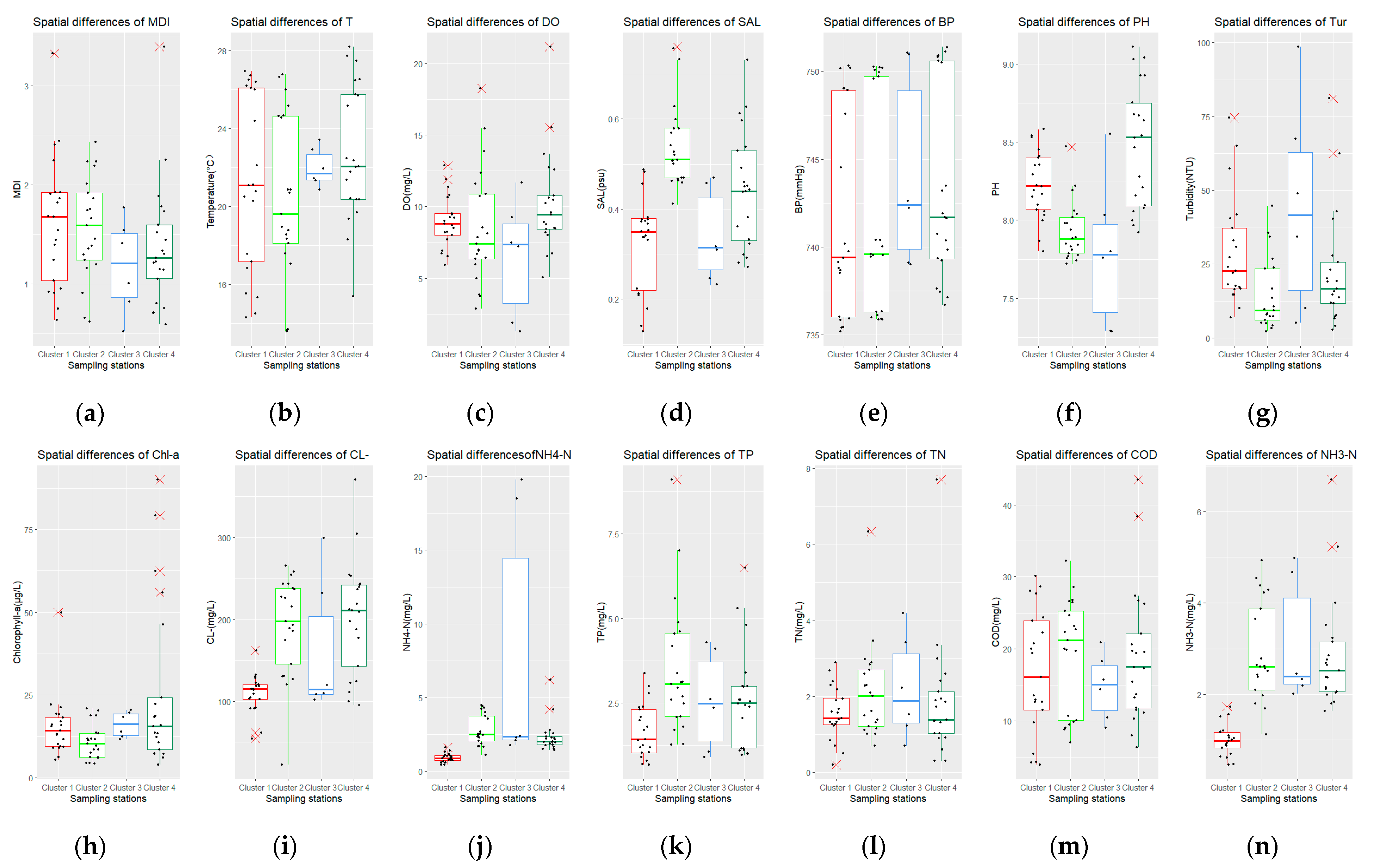
Based on the HCA, the boxplots show the spatial variation in water quality in the Majiagou River (Figure 3). Water quality factors with significant spatial differences included MDI, salinity, pH, turbidity, CL, chlorophyll-a, ammonium nitrogen, TP, TN and COD. For MDI, Clusters 1 and 2 were significantly higher than Clusters 3 and 4. The MDI in the outer suburbs of the city was similar to that in the upstream areas of the river and decreased significantly after flowing into the urban area. TN in the lower reaches (Clusters 3 and 4) was slightly higher than that in the upstream area; however, here, ammonium nitrogen was obviously higher than that in the upstream area. This phenomenon was also reflected in COD, TP and CL: all of these differences were due to human interference. The upper reaches were lower in salinity (Cluster 1, 0.22~0.38 psu) compared with the suburbs and downstream areas (Cluster 4, 0.33~0.54 psu). The pH for all the monitoring sites was alkaline, with urban reach being the highest (Cluster 4, 8.4~8.75), and the turbidity of the urban samples was higher. There was no significant difference in dissolved oxygen (DO, 7~9 mg/L).
From the spatial-temporal distribution of the water quality factors, we found that each monitoring site had ecological significance, and the characteristics regarding the ecological suitability for macro-invertebrates could be analyzed accurately.

3.2. Identification of Critical Environmental Parameters

The PCA results applied to data sets from spring, summer and autumn are shown in Table 3. We assumed that when the weight of the factor was greater than 0.9, PC had a high correlation with it (Figure 2).
In the spring, the PCA for water quality factors delivered four PCs, which, together, accounted for 80.12% of the total variance (Table 3, Figure 4). PC1 accounted for 31.6%, which had a strong positive correlation with NH4+-N. For PC2 (total variance of 24.1%) and PC3 (total variance of 14.4%), the weights for these factors were lower than 0.9, and PC4 (total variance of 10.0%), which presented a strong positive correlation with pH. This indicated that there were two critical environmental parameters (variance inflation factor between the parameters (VIF) < 10) in the spring.
In the summer, all PCs together accounted for 86.5% of the total variance (Table 3, Figure 4). PC1 accounted for 39.8%, which had a strong positive correlation with NH4+-N; PC2 (total variance of 16.7%) had a strong positive correlation with salinity and CL; PC3 (total variance of 12.3%) had a strong positive correlation with Chl-a; PC4 (total variance of 9.4%) had a strong positive correlation with TN; and for PC5 (total variance of 8.3%), all the weights for these factors were lower than 0.9. There were five critical environmental parameters (variance inflation factor between the parameters (VIF) < 10) in the summer.
In the autumn, the PCA for water quality factors delivered four PCs, which, together, accounted for 79.9% of the total variance (Table 3, Figure 4). PC1 accounted for 34.7%, which had a strong positive correlation with NH4+-N; for PC2 (total variance of 22.8%), PC3 (total variance of 13.5%) and PC4 (total variance of 8.7%), all the weights were lower than 0.9. This indicated that there was one critical environmental parameter in the autumn.
Based on the identification of all seasonal critical factors, seven environmental factors were eliminated, and a total of six critical factors entered the next step of model construction.

3.3. Response between Macro-Invertebrate MDI and Critical Quality Parameters Using GAM

3.3.1. Single-Factor Significance Test Used for Critical Water Quality Factors

The single-factor GAM model was constructed after being screened by PCA in order to test the significance of critical water quality factors and MDI (Table 4). The single-factor GAMs showed that NH4+-N, TN and Chl-a passed the significance test (p-value < 0.1); then, SAL, CL and pH were eliminated. We constructed interaction terms between NH4+-N, TN and Chl-a and confirmed that they all had high significance (p < 0.01). This result showed that the PCA and VIF test methods had strong robustness and critical environmental parameters were accurately identified. The deviance explained (DE) represented variance in the response variable explained by the model, as shown in Table 4. The DE of the interaction terms was higher than that of the single-factor test. The result of effective degree (edf) indicated MDI and NH4+-N had a strong linear relationship. In our study, we considered the interaction between these parameters and adopted a multi-factor GAM model to quantify the relationship between MDI and critical quality parameters.

3.3.2. Multi-Factor GAM Optimization

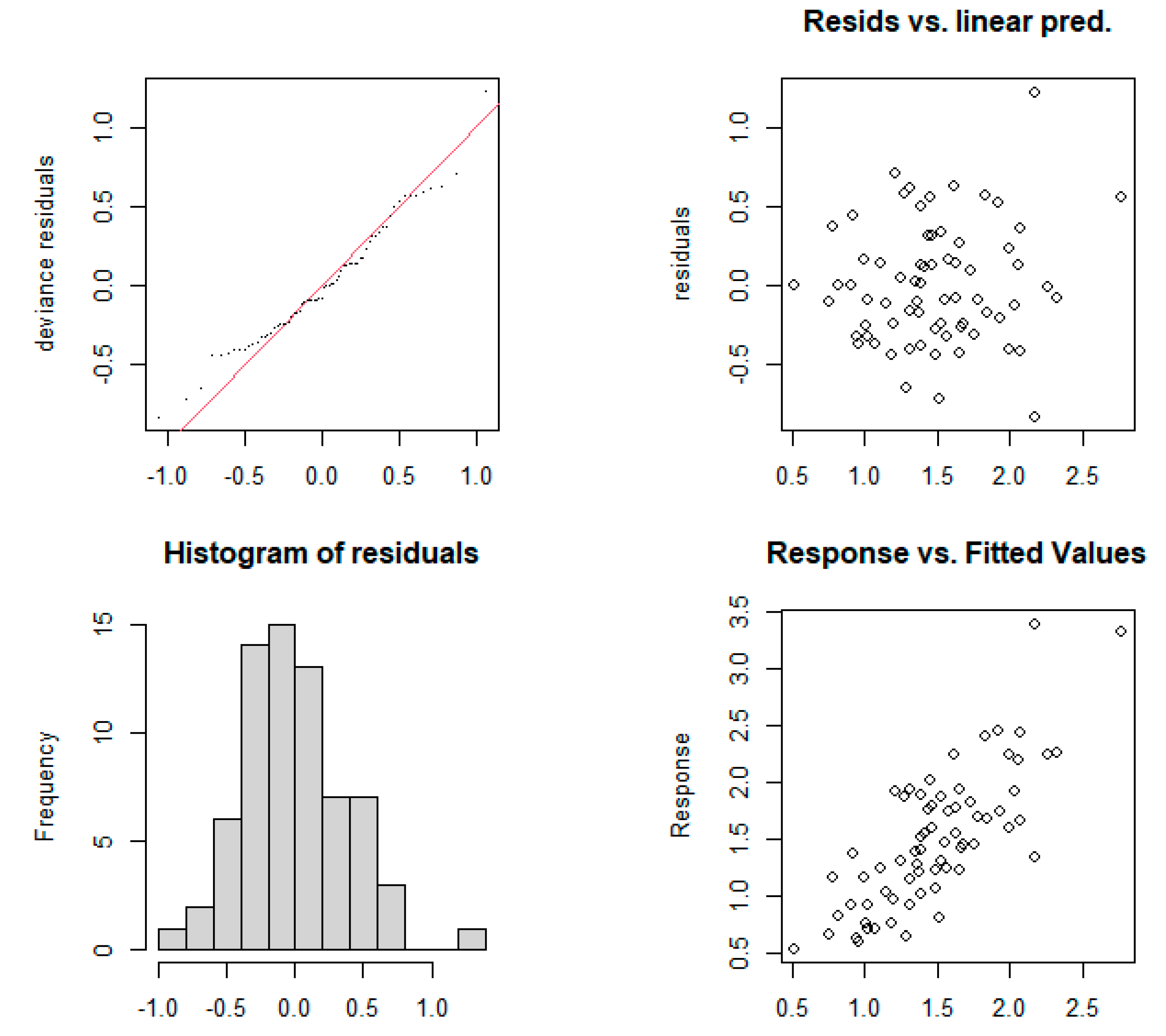
We used the final remaining three critical water quality factors to construct a GAM model (Model 1); the model results showed that it explained 52.2% of the variance. To improve the DE, we added three interaction items to the model (Model 1, 2, 3); the GAM results showed that all DE improved after the addition of interaction items, and the AICs (Akaike information criteria) of all optimization models were lower than that of Model 1 (Table 5). Among the three optimization models, Model 2 had the highest DE value, and both GCV (Generalized Cross Validation) and AIC were low; therefore, Model 2 had the highest goodness of fit and was the best model in our study. According to the histogram of model residuals, the rationality of the model was tested; Figure 5 shows that the model residuals essentially conformed to a normal distribution, and thus, the model was robust.

3.3.3. Response between MDI and Critical Quality Parameters

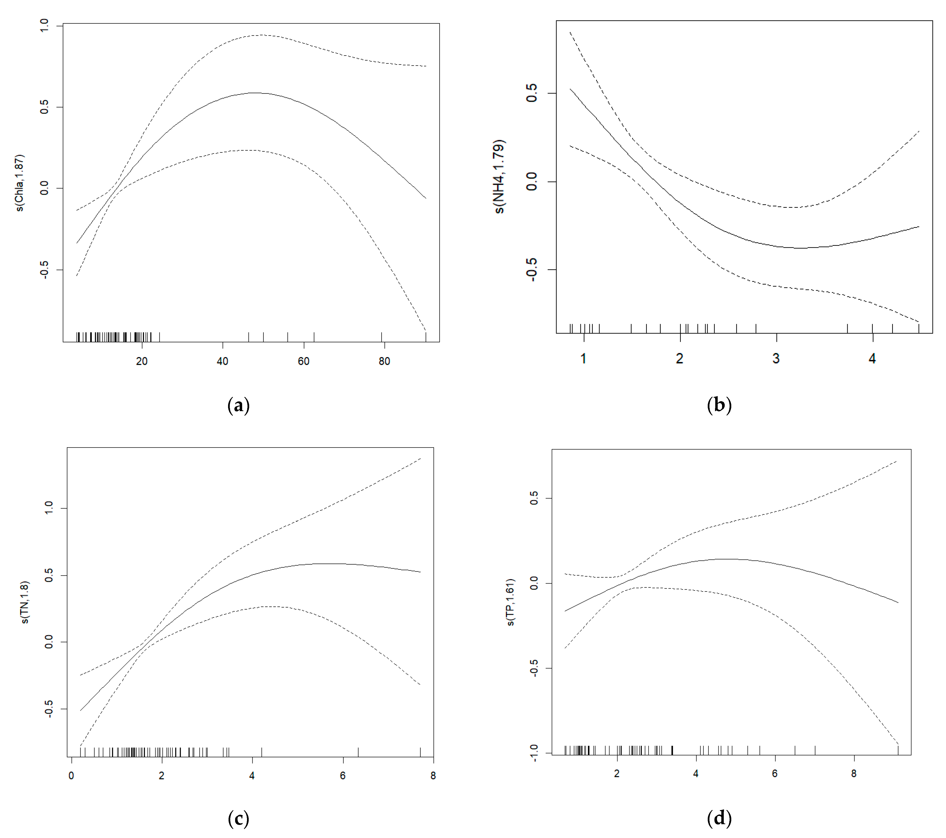
The response curves of Model 2 indicate a nonlinear relationship between the MDI and critical quality parameters (Figure 6). According to the results of the response curves: (1) The relationship between chlorophyll-a and MDI was unimodal; when the value of chlorophyll-a was less than 48, MDI was positively correlated with chlorophyll-a; conversely, there was a negative correlation when the value of chlorophyll-a was more than 48. (2) MDI and NH4+-N essentially showed a negative correlation; when NH4-N was 3.2 mg/L, MDI was at its lowest value and then rose slowly. (3) TN represented the trophic degree of the river; when the TN value reached 5.8, MDI reached its peak and then slowly declined with the increase in the total nitrogen value. (4) When MDI was higher than the mean value, the chlorophyll-a range was 18.1 μg/L~83 μg/L. NH4+-N was less than 1.8 mg/L; TN was 1.8~6.8 mg/L.
For the urban river, the eutrophication of some reaches was very serious because of human activities, especially with the accumulation of nitrogen and phosphorus at the inlet of the river. In our study, although TP was not a critical water quality factor, it had a strong correlation with TN. Therefore, a GAM model was established for TP to analyze its relationship with MDI (Figure 6). It was found that the response curve shapes of MDI on TN and TP were very similar; when the value of TP was 4.9 mg/L, MDI reached its highest value.

4. Discussion

4.1. Response of Benthic Macro-Invertebrates to Critical Water Quality Factors

In our study, beginning with the seasonal and spatial differences of environmental factors, we analyzed the critical environmental factors in each season and the spatial clustering of each monitoring site and constructed an ecological suitability model of macro-invertebrates, confirming the response of macro-invertebrates to the critical environmental factors, and finally determining the ecological threshold for critical water quality factors. Combined with the HCA results of these sites, this study provides an important reference for habitat management in different reaches.
Macro-invertebrates have a unique ecological niche in rivers and are sensitive to changes in water quality environmental factors; thus, MDI is regulated by environmental factors. In previous studies on macro-invertebrates in urban rivers, it was believed that water quality factors had potential impacts on benthic fauna, especially regarding the levels of nutrients such as total phosphorus and total nitrogen, which limited the survival of macro-invertebrates and led to the niche loss of macro-invertebrates [40]. However, due to the differences in study areas, the environmental factors that played key roles in the habitats of macro-invertebrates varied by situation; with different degrees of human disturbance, the basic hydrological conditions of urban rivers varied greatly, leading to changes in some limiting factors. For example, previous studies have shown that dissolved oxygen (DO) has a negative effect on macro-invertebrates [41], but due to the shallow water depth, fast velocity and low plankton density at some monitoring sites, the level of DO was high, and this was not a limiting factor for macro-invertebrates in the Majiagou River. Blanka Gal et al. (2020) undertook an interesting study in Europe on benthic fauna at a typical site of urbanization (road crossings), and an assessment of environmental variables showed that road crossings caused habitat changes; it was suggested that these changes were the main drivers of biodiversity patterns. However, Luciana Irene Gallardo et al. (2019) showed that seven benthic indices were responsive to urbanization, and benthic community structures were similar to different levels of anthropogenic disturbances in Argentina. In our study, some sampling points were also involved in road crossings, and it was confirmed that human disturbance had a certain effect on the benthic community structure, which was contrary to the study in Argentina, probably because the ecosystem of the Majiagou River is severely shaped by human disturbance, the river length is longer, and the environmental factors are different from those of lakes.
The same situation also occurred for water temperature environmental factors; the spatial difference analysis of the monitoring sites after HCA showed that spatial differences in water temperature environmental factors were not significant because the Majiagou River was small scale and the samplings were carried out over the same time period. Shen et al. (2022) considered salinity to be the most important factor affecting macro-invertebrate biodiversity and identified a positive correlation [42]. The results of a one-way ANOVA of environmental factor seasonality differences confirmed that the seasonal variation in salinity in our study was not significant, and it was difficult to judge the coupling relationship between salinity and macro-invertebrates. In conclusion, the study on the response of macro-invertebrates to environmental factors needed to consider the actual situation of rivers.
For urban rivers, we should not only consider the potential impact of nutrients on diversity but also consider the coupling relationship between the interactions of various critical environmental factors and the macro-invertebrate community [43]. In our study, we determined the ecological suitability of benthic animals by fitting the responses of critical environmental factors and macro-invertebrates and demonstrated that benthic responses to multiple critical environmental factors were nonlinear, confirming the findings of previous studies [44,45]. We found that under human disturbances, the density of pollution-resistant species such as chironomid larvae and oligochaetes increased exponentially and that in such circumstances, the benthic community became homogenized. Finally, based on the response characteristics of macro-invertebrates to these critical factors, we could determine ecological suitability for species survival.

4.2. Construction of GAM Model Based on HCA and PCA

When there are too many monitoring sites, the analysis process always becomes more complicated. HCA can effectively cluster the sites with the same characteristics [46]. Excessive numbers of environmental factors reduce the weight of critical factors, leading to data redundancy [47]; however, we achieved a data dimension reduction through PCA, expecting to interpret target variables with the smallest amount of variable interaction. Using PCA, VIF and a significance test (p-value < 0.1), we finally selected three critical water quality parameters from thirteen environmental factors, reducing data redundancy by 76.9%, which provided a basis for more accurately determining the response of species to critical factors. GAM could fit the nonlinear relationship robustly, which was valuable for the quantitative study of species’ niche requirements. In our study, the GAM model was used to analyze macro-invertebrate responses to environmental parameters and accounted for 60% of species diversity differences. In conclusion, the GAM model based on HCA and PCA could effectively improve the robustness of the model and provide references for macro-invertebrate habitat suitability evaluation.

4.3. The Limitations and Prospects of Our Study

In our study, a GAM model based on HCA and PCA was used to analyze the ecological suitability of urban rivers for benthic fauna. The study showed that it had high robustness but that further studies were still needed in the future. (1) As a part of the food web of aquatic organisms, a study of macro-invertebrates could be combined with a study of the plankton community to carry out more comprehensive and in-depth research. (2) Our study used a GAM model to quantify the response of MDI to critical environmental factors; if various functional groups or species composition need to be considered, CCA or RDA could be used. (3) The problem of overfitting could also be solved by increasing the sample size. (4) For urban rivers, we could pay attention to the nutrient concentration in the sediment and the influence of river channel hardening so as to better support the ecological suitability study of benthic macro-invertebrate habitats.

5. Conclusions

In our study, one-way ANOVA and HCA were used to explain the spatiotemporal differences in water environmental factors in the Majiagou River. PCA was used to reduce data redundancy, identify critical factors, and in constructing a GAM model of macro-invertebrates and critical factors, we confirmed the ecological threshold for benthic organisms. The main conclusions were as follows:
  • The macro-invertebrate community in the Majiagou River had differences in their spatiotemporal distribution. Due to human disturbance, the macro-invertebrate community tended to be homogeneous and resistant to pollution, with a decrease in the biodiversity index.
  • In this study, one-way ANOVA and hierarchical cluster analysis (HCA) were used to analyze the temporal and spatial variations in water quality factors in the Majiagou Watershed. The results showed that COD in the Majiagou River had obvious seasonal differences, and the water quality in different reaches had spatial distribution differences; CL, NH4+-N, TP, TN and COD in the downstream area were higher than they were in the upstream area.
  • Principal component analysis was used to identify the key water environmental factors and three environmental factors with a significant impact on benthic animals were finally selected through a significance test, which reduced data redundancy.
  • A GAM model fitted the nonlinear relationship between MDI and critical water environmental factors and fitted the response curve for the critical environmental factors and macro-invertebrates. This could be used to further analyze ecological suitability. The purpose of our study was to provide a reference for the integrated management of urban river water ecosystems.

Author Contributions

Funding acquisition, H.Y.; Investigation, Y.Z., H.Y., W.D., T.X. and Y.G.; Methodology, Y.Z., H.Y., M.L., J.L. and Y.W.; Resources, H.Y.; Writing—review and editing, Y.Z., H.Y., M.L. and J.L. All authors have read and agreed to the published version of the manuscript.

Funding

This study was funded by the National Key R&D Program of China. (No. 2022YFF1300903).

Data Availability Statement

Not applicable.

Conflicts of Interest

The authors declare no conflict of interest.

References

  1. Beißler, H. A Combined Field and Remote-Sensing based Methodology to Assess the Ecosystem Service Potential of Urban Rivers in Developing Countries. Remote Sens. 2019, 11, 1697. [Google Scholar] [CrossRef] [Green Version]
  2. Begum, W.; Goswami, L.; Sharma, B.-B.; Kushwaha, A. Assessment of urban river pollution using the water quality index and macro-invertebrate community index. Environ. Dev. Sustain. 2022, 1–26. [Google Scholar] [CrossRef]
  3. Edegbene, A.O.; Odume, O.N.; Arimoro, F.O.; Keke, U.N. Identifying and classifying macroinvertebrate indicator signature traits and ecological preferences along urban pollution gradient in the Niger Delta. Environ. Pollut. 2021, 281, 117076. [Google Scholar] [CrossRef]
  4. Wei, C.; Gao, C.; Han, D.; Zhao, W.; Lin, Q.; Wang, G. Spatial and Temporal Variations of Water Quality in Songhua River from 2006 to 2015: Implication for Regional Ecological Health and Food Safety. Sustainability 2017, 9, 1502. [Google Scholar] [CrossRef] [Green Version]
  5. Sterling, J.-L.; Rosemond, A.-D.; Wenger, S.-J. Watershed urbanization affects macroinvertebrate community structure and reduces biomass through similar pathways in Piedmont streams, Georgia, USA. Freshw. Sci. 2016, 35, 676–688. [Google Scholar] [CrossRef] [Green Version]
  6. Gál, B.; András, W.; János, F.; Schmera, D. The effects of road crossings on stream macro-invertebrate diversity. Biodivers. Conserv. 2020, 29, 729–745. [Google Scholar] [CrossRef] [Green Version]
  7. Gallardo, L.-I.; Juan-Manuel, C.; Alicia-Susana-Guadalupe, P. Urban rain-fed lakes: Macro-invertebrate assemblages associated with Egeria najas as indicators of biological integrity in wetlands of Corrientes Province (Argentina). Biodivers. Conserv. 2019, 28, 1549–1568. [Google Scholar] [CrossRef]
  8. Andem, A.B.; Ibor, O.R.; Oku, E.E.; Ekanem, S.B.; Chukwuka, A.V.; Adeogun, A.O. Urbanisation gradients, riparian-loss and contaminant effects on macroinvertebrate distribution within a tropical river (Nigeria). Chem. Ecol. 2022, 38, 503–526. [Google Scholar] [CrossRef]
  9. Van Damme, P.-A.; Caroli, H.; Alfredo, A.; Bervoets, L. Macroinvertebrate community response to acid mine drainage in rivers of the High Andes (Bolivia). Environ. Pollut. 2008, 156, 1061–1068. [Google Scholar] [CrossRef]
  10. Arimoro, F.O.; Odume, O.N.; Uhunoma, S.I.; Edegbene, O.A. Anthropogenic impact on water chemistry and benthic macroinvertebrate associated changes in a southern Nigeria stream. Environ. Monit. Assess. 2015, 187, 1–14. [Google Scholar] [CrossRef]
  11. Belle, G.; Fossey, A.; Esterhuizen, L. Use of multiple indicators to assess the pollution condition of urban streams: A case study of Bloemspruit, Free State Province, South Africa. Water Environ. J. 2020, 34, 93–105. [Google Scholar] [CrossRef]
  12. Aazami, J.; Maghsodlo, H.; Mira, S.S.; Valikhani, H. Health evaluation of riverine ecosystems using aquatic macroinvertebrates: A case study of the Mohammad-Abad River, Iran. Int. J. Environ. Sci. Technol. 2020, 17, 2637–2644. [Google Scholar] [CrossRef]
  13. Blocksom, K.A.; Kurtenbach, J.P.; Klemm, D.J.; Fulk, F.A.; Cormier, S.M. Development and evaluation of the lake Macroinvertebrate Integrity Index (lmii) for New Jersey Lakes and Reservoirs. Environ. Monit. Assess. 2001, 77, 311–333. [Google Scholar] [CrossRef] [PubMed]
  14. Pecher, C.; Fritz, S.A.; Marini, L.; Fontaneto, D.; Pautasso, M. Scale-dependence of the correlation between human population and the species richness of stream macro-invertebrates. Basic Appl. Ecol. 2010, 11, 272–280. [Google Scholar] [CrossRef]
  15. Zhang, J.; Tang, Y.; Kou, Z.; Teng, X.; Cai, W.; Hu, J. Shift of Sediments Bacterial Community in the Black-Odor Urban River during In Situ Remediation by Comprehensive Measures. Water 2019, 11, 2129. [Google Scholar] [CrossRef] [Green Version]
  16. Mitchell, E.-G.; Whittle, R.-J.; Griffiths, H.-J. Benthic ecosystem cascade effects in Antarctica using Bayesian network inference. Commun. Biol. 2020, 3, 582. [Google Scholar] [CrossRef]
  17. Yang, L.; Peng, S.; Sun, J.; Zhao, X.; Li, X. A case study of an enhanced eutrophication model with stoichiometric zooplankton growth sub-model calibrated by Bayesian method. Environ. Sci. Pollut. Res. 2016, 23, 8398–8409. [Google Scholar] [CrossRef]
  18. Cao, Y.; Cummings, K.; Hinz, L.; Douglass, S.A.; Stodola, A.P.; Holtrop, A.M. Reconstructing the natural distribution of individual unionid mussel species and species diversity in wadeable streams of Illinois, USA, with reference to stream bioassessment. Freshw. Sci. 2017, 36, 669–682. [Google Scholar] [CrossRef]
  19. Li, X.; Yu, H.; Wang, H.; Ma, C. Phytoplankton community structure in relation to environmental factors and ecological assessment of water quality in the upper reaches of the Genhe River in the Greater Hinggan Mountains. Environ. Sci. Pollut. Res. 2019, 26, 17512–17519. [Google Scholar] [CrossRef]
  20. Sun, X.; Mwagona, P.C.; Shabani, I.E.; Hou, W.; Li, X.; Zhao, F.; Chen, Q.; Zhao, Y.; Liu, D.; Li, X.; et al. Phytoplankton functional groups response to environmental parameters in Muling River basin of northeast China. Ann. Limnol.-Int. J. Limnol. 2019, 55, 17. [Google Scholar] [CrossRef] [Green Version]
  21. Arias, M.J.; Vaschetto, P.A.; Marchese, M.; Regaldo, L.; Gagneten, A.M. Benthic Macroinvertebrates and Zooplankton Communities as Ecological Indicators in Urban Wetlands of Argentina. Sustainability 2022, 14, 4045. [Google Scholar] [CrossRef]
  22. Cui, S.; Zhang, F.; Hu, P.; Hough, R.; Fu, Q.; Zhang, Z.; An, L.; Li, Y.-F.; Li, K.; Liu, D.; et al. Heavy Metals in Sediment from the Urban and Rural Rivers in Harbin City, Northeast China. Int. J. Environ. Res. Public Health 2019, 16, 4313. [Google Scholar] [CrossRef] [PubMed] [Green Version]
  23. Razmkhah, H.; Abrishamchi, A.; Torkian, A. Evaluation of spatial and temporal variation in water quality by pattern recognition techniques: A case study on Jajrood River (Tehran, Iran). J. Environ. Manag. 2010, 91, 852–860. [Google Scholar] [CrossRef] [PubMed]
  24. Passos JB DM, C.; Teixeira DB, D.S.; Campos, J.A.; Lima RP, C.; Fernandes-Filho, E.I.; da Silva, D.D. Multivariate statistics for spatial and seasonal quality assessment of water in the Doce River basin, Southeastern Brazil. Environ. Monit. Assess. 2021, 193, 125. [Google Scholar] [CrossRef] [PubMed]
  25. Bertossi AP, A.; de Menezes JP, C.; Cecílio, R.A.; Garcia GD, O.; Neves, M.A. Selection and grouping of indicators of water quality using Multivariate Statistics. Semin.-Cienc. Agrar. 2013, 34, 2025–2036. [Google Scholar]
  26. Konishi, T. Principal component analysis for designed experiments. BMC Bioinform. 2015, 16, 1–9. [Google Scholar] [CrossRef] [Green Version]
  27. Wang, H.; Xu, Y.; Sulong, R.S.; Ma, H.; Wu, L. Comprehensive Evaluation of Water Carrying Capacity in Hebei Province, China on Principal Component Analysis. Front. Environ. Sci. 2021, 9. [Google Scholar] [CrossRef]
  28. Khatri, N.; Raval, K.; Jha, A. Integrated water quality monitoring of Mahi river using benthic macroinvertebrates and comparison of its biodiversity among various stretches. Appl Water Sci. 2021, 11, 143. [Google Scholar] [CrossRef]
  29. Salmeron, R.; Garcia, C.-B.; Garcia, J. Variance Inflation Factor and Condition Number in multiple linear regression. J. Stat. Comput. Simul. 2018, 88, 2365–2384. [Google Scholar] [CrossRef]
  30. Thompson, C.G.; Kim, R.S.; Aloe, A.M.; Becker, B.J. Extracting the Variance In flation Factor and Other Multicollinearity Diagnostics from Typical Regression Results. Basic Appl. Soc. Psychol. 2017, 39, 81–90. [Google Scholar] [CrossRef]
  31. Chauhan, N.; Paliwal, R.; Kumar, V.; Kumar, S.; Kumar, R. Watershed Prioritization in Lower Shivaliks Region of India Using Integrated Principal Component and Hierarchical Cluster Analysis Techniques: A Case of Upper Ghaggar Watershed. J. Indian Soc. Remote Sens. 2022, 50, 1051–1070. [Google Scholar] [CrossRef]
  32. Hua, A.; Kusin, F.; Praveena, S. Spatial Variation Assessment of River Water Quality Using Environmetric Techniques. Pol. J. Environ. Stud. 2016, 25, 2411–2421. [Google Scholar] [CrossRef] [PubMed]
  33. Pärn, J.; Verhoeven, J.T.; Butterbach-Bahl, K.; Dise, N.B.; Ullah, S.; Aasa, A.; Egorov, S.; Espenberg, M.; Järveoja, J.; Jauhiainen, J.; et al. Nitrogen-rich organic soils under warm well-drained conditions are global nitrous oxide emission hotspots. Nat. Commun. 2018, 9, 1135. [Google Scholar] [CrossRef] [Green Version]
  34. Vázquez, R.; Vimos-Lojano, D.; Hampel, H. Habitat Suitability Curves for Freshwater Macroinvertebrates of Tropical Andean Rivers. Water 2020, 12, 2703. [Google Scholar] [CrossRef]
  35. Su, Y.; Li, W.; Liu, L.; Li, J.; Sun, X.; Hu, W. Assessment of medium and small river health based on macroinvertebrates habitat suitability curves: A case study in a tributary of Yangtze River, China. Water Policy 2020, 22, 602–621. [Google Scholar] [CrossRef]
  36. Gutiérrez-Estrada, J.C.; Bilton, D.T. A heuristic approach to predicting water beetle diversity in temporary and fluctuating waters. Ecol. Model. 2010, 221, 1451–1462. [Google Scholar] [CrossRef] [Green Version]
  37. Zhang, H.; Huo, S.; Yeager, K.M.; Li, C.; Xi, B.; Zhang, J.; He, Z.; Ma, C. Apparent relationships between anthropogenic factors and climate change indicators and POPs deposition in a lacustrine system. J. Environ. Sci. 2019, 83, 83174–83182. [Google Scholar] [CrossRef]
  38. Jiang, Y.; He, K.; Li, Y.; Qin, M.; Cui, Z.; Zhang, Y.; Yao, Y.; Chen, X.; Deng, M.; Gray, A.; et al. Driving Factors of Total Organic Carbon in Danjiangkou Reservoir Using Generalized Additive Model. Water 2022, 14, 891. [Google Scholar] [CrossRef]
  39. Downie, A.-L.; von Numers, M.; Boström, C. Influence of model selection on the predicted distribution of the seagrass Zostera marina. Estuar. Coast. Shelf Sci. 2013, 121, 8–19. [Google Scholar] [CrossRef]
  40. Yang, Y.; Yi, Y.; Zhou, Y.; Wang, X.; Zhang, S.; Yang, Z. Spatio-temporal variations of benthic macroinvertebrates and the driving environmental variables in a shallow lake. Ecol. Indic. 2020, 110, 105948. [Google Scholar] [CrossRef]
  41. Bednarek, A.-T.; Hart, D.-D. Modifying dam operations to restore rivers: Ecological responses to Tennessee river dam mitigation. Ecol. Appl. 2005, 15, 997–1008. [Google Scholar] [CrossRef] [Green Version]
  42. Shen, Z.; Yang, Y.; Ai, L.; Yu, C.; Su, M. A hybrid CART-GAMs model to evaluate benthic macroinvertebrate habitat suitability in the Pearl River Estuary, China. Ecol. Indic. 2022, 143, 143109368. [Google Scholar] [CrossRef]
  43. Muvengwi, J.; Chikorowondo, G.; Mbiba, M.; Gandiwa, E. Diversity and abundance of macro-invertebrates on abandoned cattle kraals in a semi-arid savanna. Ecol. Evol. 2018, 8, 8477–8489. [Google Scholar] [CrossRef] [PubMed]
  44. Aspin, T.W.H.; Khamis, K.; Matthews, T.; Milner, A.M.; O’callaghan, M.J.; Trimmer, M.; Woodward, G.; Ledger, M.E. Extreme drought pushes stream invertebrate communities over functional thresholds. Glob. Chang. Biol. 2018, 25, 230–244. [Google Scholar] [CrossRef] [PubMed]
  45. Hwang, S.A.; Hwang, S.J.; Park, S.R.; Lee, S.W. Examining the Relationships between Watershed Urban Land Use and Stream Water Quality Using Linear and Generalized Additive Models. Water 2016, 8, 155. [Google Scholar] [CrossRef] [Green Version]
  46. Torres, S.H.; Martin, J.P.; Gárgano, L.; Armendáriz, L.C. Análisis de la calidad ambiental en un sector del Río Chico (Santa Cruz, Argentina) basado en bioindicadores bentónicos. Inf. Científicos Técnicos-UNPA 2019, 11, 36–49. [Google Scholar] [CrossRef]
  47. Colla, M.-F.; Cesar, I.-I.; Salas, L.-B. Benthic insects of the El Tala River (Catamarca, Argentina): Longitudinal variation of their structure and the use of insects to assess water quality. Braz. J. Biol. 2013, 73, 357–366. [Google Scholar] [CrossRef] [PubMed] [Green Version]
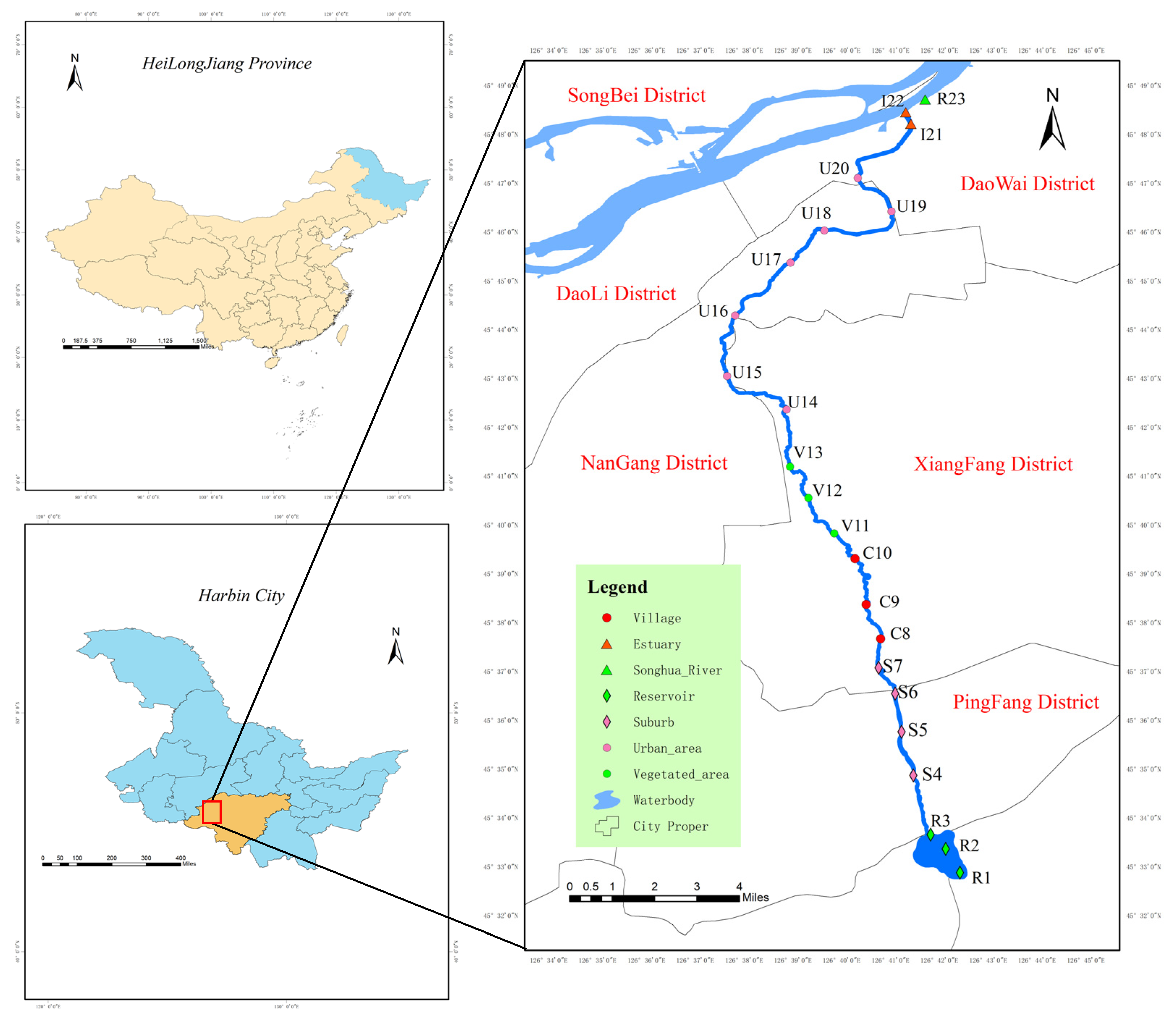
Figure 1. Study area and sampling points location.
Water 15 02269 g001
Figure 2. (a) Sum of squared error (SSE) method used to determine the optimal number of clusters. (b) Dendrogram presenting the clusters of sampling stations.
Water 15 02269 g002
Figure 3. Boxplots of water quality factors in different Clusters: MDI (a), Temperature (b), DO (c), SAL (d), BP (e), pH (f), Turbidity (g), Chl-a (h), CL- (i), NH4+-N (j), TP (k), TN (l), COD (m), NH3-N (n).
Water 15 02269 g003
Figure 4. PCs component plot in rotated space for spring (a), summer (b) and autumn (c) water parameters, respectively (component plot in 3D rotated space showing all three components).
Water 15 02269 g004
Figure 5. Residual analysis of optimal model structure.
Water 15 02269 g005
Figure 6. The response curves of quality parameters: (a) Chlorophyll-a (b) NH4+-N (c) TN (d) TP.
Water 15 02269 g006
Table 1. Macrobenthos community composition in different seasons in the Majiagou River.
SeasonPhylumClassSpecies
SpringArthropodaInsectaChinonomus pallidivittatus
Dicrotendipes tritomus
Chironomus riparius
MalacostracaExopalaemon modestus
ClitellataGlossiphonia lata
AnnelidaOligochaetaLimnodrilus hoffmeisteri
Tubifex tubifex
MolluscaGastropodaBithynia fuchsiana
LamellibranchiaSphaerium lacustre
NemathelminthesGordiacea
SummerArthropodaInsectaDicrotendipes lobifer
Glyptotendipes cauliginellus
MalacostracaExopalaemon modestus
ClitellataHelobdella nuda
AnnelidaOligochaetaLimnodrilus hoffmeisteri
Tubifex tubifex
MolluscaGastropodaRadix swinhonei
Bithynia fuchsiana
LamellibranchiaSphaerium lacustre
NemathelminthesGordiacea
AutumnArthropodaInsectaCricotopus sylvestris
Chinonomus pallidivittatus
Dicrotendipes tritomus
MalacostracaExopalaemon modestus
ClitellataHelobdella stagnalis
AnnelidaOligochaetaBranchiura sowerbyi
Limnodrilus hoffmeisteri
Tubifex tubifex
MolluscaGastropodaRadix swinhonei
Bithynia fuchsiana
LamellibranchiaSphaerium lacustre
NemathelminthesGordiacea
Table 2. Effects of seasonal variation in water quality factors; the significant effect of seasonal variation on the index (p < 0.05) is in bold. (The significant post hoc results (p < 0.05) based on Fisher’s LSD test are shown with different lowercase letters).
SeasonEffects of Season
MayJulySeptemberStatisticsp-Value
COD22.73 ± 7.25 a20.13 ± 6.79 a11.3 ± 6.48 bF = 17.59<0.001
Salinity0.39 ± 0.12 ab0.48 ± 0.16 a0.41 ± 0.11 aF = 2.8960.062
pH8.16 ± 0.28 a8.17 ± 0.48 a8.19 ± 0.39 aF = 0.0310.97
Table 3. (a) PCA results applied to dataset in the spring; PCs together accounted for 80.1% of the total variance. (b) PCA results applied to dataset in the summer; PCs together accounted for 86.5% of the total variance. (c) PCA results applied to dataset in the autumn; PCs together accounted for 79.8% of the total variance.
PCInitial Eigenvalues
Total% of VarianceCumulative %
(a)
PC14.10831.60431.604
PC23.12724.05355.657
PC31.87714.43670.093
PC41.30310.02580.118
(b)
PC15.17739.82339.823
PC22.16416.64856.471
PC31.60312.33268.802
PC41.2229.40178.203
PC51.0758.27386.476
(c)
PC14.51734.74334.743
PC22.97022.84357.586
PC31.75413.49171.077
PC41.1378.74579.822
Table 4. Single-factor and interaction term GAM models significance test (* p < 0.1, ** p < 0.01, *** p < 0.001).
GAM Modeledfp-ValueGCVDeviance Explained (DE)Significance
MDI~s (NH4+-N, k = 3)10.0278 *0.347987.02%
MDI~s (TN, k = 3)1.80.000843 ***0.3031920.9%
MDI~s (SAL, k = 3)1.7530.1180.354167.48%×
MDI~s (Chl-a, k = 3)1.8730.00632 **0.3247415.5%
MDI~s (CL, k = 3)1.520.4450.367753.26%×
MDI~s (pH, k = 3)1.2140.9010.373910.73%×
MDI~te (NH4+-N, TN, k = 3)5.1870.00219 **0.3045128.5%
MDI~te (NH4+-N, Chl-a, k = 3)4.7510.00187 **0.3047327.4%
MDI~te (TN, Chl-a, k = 3)4.7658.8 × 10−5 ***0.2665936.5%
Table 5. GAM model of critical water quality factors and optimal structures.
GAM ModelGCVAICDeviance Explained (DE)DE Variation with Model 1
Model 1: MDI~s (TN) + s (NH4+-N) + s (Chl-a)0.24899.2083652.2%
Model 2: MDI~s (TN) + s (NH4+-N) + s (Chl-a) + te (NH4+-N, TN)0.2463796.268860%+7.8%
Model 3: MDI~s (TN) + s (NH4+-N) + s (Chl-a) + te (NH4+-N, Chl-a)0.2445797.2607356.2%+4%
Model 4: MDI~s (TN) + s (NH4) + s (Chl-a) + te (TN, Chl-a)0.2484796.9357259.4%+7.2%
Disclaimer/Publisher’s Note: The statements, opinions and data contained in all publications are solely those of the individual author(s) and contributor(s) and not of MDPI and/or the editor(s). MDPI and/or the editor(s) disclaim responsibility for any injury to people or property resulting from any ideas, methods, instructions or products referred to in the content.