Article

The Influence of Meteorological Variables on Reference Evapotranspiration Based on the FAO P-M Model—A Case Study of the Taohe River Basin, NW China

College of Water Conservancy and Hydropower Engineering, Gansu Agricultural University, Lanzhou 730070, China
*
Author to whom correspondence should be addressed.
Water 2023, 15(12), 2264; https://doi.org/10.3390/w15122264
Submission received: 11 May 2023 / Revised: 6 June 2023 / Accepted: 14 June 2023 / Published: 16 June 2023
(This article belongs to the Section Hydrology)

Abstract

:
To explore the mechanisms driving variation in ET0 (reference evapotranspiration) in an arid inland region of Northwest China, daily meteorological data from 1960 to 2019 from 19 meteorological stations in the Taohe River basin and its surrounding areas were used to analyze the temporal and spatial distributions of ET0 and meteorological variables. Various qualitative and quantitative analysis methods were used to reveal the correlation between ET0 and meteorological variables. The degree of sensitivity of ET0 variations to meteorological variables and the contribution from each meteorological variable were clarified, and the mechanisms driving variation in ET0 were fully revealed. These are the results: (1) ET0 in the Taohe River basin presented a significant upward trend with a linear change rate of 0.93 mm/a, and a sudden change occurred in 1994. The spatial variation in ET0 ranged from 779.8 to 927.6 mm/a, with low values in the upper and middle reaches and high values in the lower reaches. The ET0 at 14 stations (73.68% of the total) was significantly increased (p < 0.05), and that at 5 stations (26.32% of the total) was not significantly increased (p > 0.05). (2) RH, Rn, and u2 did not change significantly, while Tmax and Tmin showed a significant upward trend. (3) Rn is a meteorological variable closely related to variations in ET0, and is the most sensitive variable for variations in ET0, followed by Tmax and u2. (4) Tmax is the meteorological variable that contributes most to the variation in ET0 (30.98%), followed by Tmin (29.11%), u2 (6.57%), Rn (2.22%), and RH (0.05%). The research results provide a scientific basis for the rational and efficient utilization of water resources and the maintenance of ecosystem health.

1. Introduction

As an important link in the process of the hydrologic cycle, evapotranspiration promotes the continuous flux and conversion of water and energy in the three surface layers, the pedosphere, biosphere, and atmosphere [1], and constitutes a central link in the climate system. Variations in evapotranspiration have a strong impact on hydrological processes [2], and this is a popular field of multidisciplinary research in the context of climate change [3]. Reference evapotranspiration (ET0) represents the evapotranspiration of a hypothetical grass reference crop with specific characteristics [4], which significantly affects the availability of water resources [5]. It is often used to estimate crop evapotranspiration [6,7] and develop effective irrigation plans to ensure agricultural productivity [8]. The multitype drought index considers ET0 as an important input variable, which is the key to accurately monitoring and alerting to drought conditions [9]. In the context of global warming, increasing variations in ET0 aggravate the frequency, intensity, and duration of drought [10]. Therefore, the study of ET0 is of great significance for ensuring the water use efficiency of ecosystems, for efficiently utilizing water resources, and for monitoring the water and heat status of the surface [1,8]. Owing to the interactions among atmosphere–vegetation–surface systems, various factors such as meteorological conditions and underlying surface characteristics affect the variation in ET0 [11,12]. According to the FAO P-M model, ET0 is calculated by temperature, relative humidity, wind speed, sunshine duration, and geographical location [13,14]. Any change in these variables may trigger a change in ET0, and the interaction among various meteorological factors is relatively complex [15,16]. In the context of global warming, it is helpful to quantitatively study the spatiotemporal variation in ET0 and the interaction between meteorological factors, to explore the sensitivity of ET0 to variation in different meteorological factors and to identify the influence of various climate variables to reveal the response mechanism of hydrological processes to climate change [17].
Some valuable research has been conducted on ET0 estimation and its spatiotemporal variation, driving mechanisms, and influence [2,18,19,20,21]. Dinpashoh et al. [22] used the Mann–Kendall method and Sen’s estimator method to analyze monotonic trends in ET0 in the Lake Urmieh basin. Di Nunno et al. [23] compared the reference evapotranspiration predicted by machine learning algorithms with the evapotranspiration calculated for two climate scenarios, RCP 4.5 and RCP 8.5, and predicted future trends in ET0. Jerin et al. [24] used a modified Mann–Kendall test, wavelet analysis, and kriging models to study the spatiotemporal variation in ET0 and used linear regression analysis and partial correlation coefficients to identify the factors controlling these variations. Fu et al. [25] constructed multiple linear regression equations for temperature, precipitation, sunshine duration, wind speed, and relative humidity with terrestrial evapotranspiration (ET) to determine climatic factors on ET. Jiang et al. [26] obtained the contribution of climate variables to ET0 variation by multiplying the sensitivity coefficients of individual climate variables by their relative change. The relevant studies used statistical analysis, the Sobol method, sensitivity analysis, and contribution rate analysis together with a variety of analytical methods that are applicable for this research [15,26,27]. Considering the numerous factors affecting the variation in ET0 and the complex interactions among meteorological factors, the combined application of multiple methods is very important to reveal the qualitative and quantitative relationship between ET0 and meteorological factors. In this paper, various methods, such as correlation coefficient, grey correlation degree, path analysis, elasticity coefficient, and contribution rate calculations, are exploratively combined in a way that has rarely been previously performed. As a transitional basin between the Qinghai–Tibet Plateau and Loess Plateau and with its heterogeneity of climate and surface conditions, the Taohe River basin in China is one of the most sensitive regions to climate change [28], but little research has been done on ET0 in the Taohe River basin [2,18,19,20,21,28]. By integrating qualitative analysis and quantitative analysis, the internal relationship and the degree of correlation between ET0 variations and meteorological factors are analyzed in a more comprehensive and objective way. The key leading factors are identified, and the sensitivity of ET0 variations to meteorological variables and the contribution from each meteorological variable are determined to reveal the mechanisms influencing ET0 variations. This study can provide a new idea to reveal the mechanisms influencing ET0 variations by combining qualitative and quantitative methods to predict more scientifically the impact of ET0 variations on hydrological processes under climate change, and complement the regional studies on ET0 in the Taohe River basin.
This research has three purposes: (1) Use the multivariate statistical method and Thiessen polygon weighted method to analyze the variations and change point in ET0 and meteorological variables in a basin and use the spatial interpolation method to determine the spatial distribution of ET0. (2) Based on qualitative analysis methods such as the correlation coefficient, grey correlation degree and path analysis, reveal close correlation between ET0 variations and meteorological variables. (3) Using quantitative analysis methods such as the elasticity coefficient and contribution rate calculation, explore the sensitivity of ET0 variations to meteorological variables and the contribution from each meteorological variable.

2. Materials and Methods

2.1. Study Area

The Taohe River is a first-level tributary on the right bank of the upper Yellow River. Originating from Xiqingshan, Qinghai Province, it flows into the Liujiaxia Reservoir in the upper main stream of the Yellow River, with a total length of 673 km and a watershed area of 25,527 km2. Its geographical location is 101°36’~104°20’ E, 34°06’~36°01’ N (Figure 1). The upper reaches are above the Xiabagou hydrological station, the middle reaches extend from the Xiabagou hydrological station to Lijiacun hydrological station, and the lower reaches are below the Lijiacun hydrological station to Hekou hydrological station. The multiyear average annual temperature increases from 1 °C in the upper reaches to 9 °C in the lower reaches, while the multiyear average annual precipitation decreases from 650 to 300 mm [29]. The upper and middle reaches are cold and humid, while the lower reaches are warm and arid [28]. The basin contains abundant water resources with large amounts of runoff in the Gansu section of the Yellow River basin. The land spans three major geomorphic units: the plateau region in the upper reaches, the alpine valley region in the middle reaches, and the loess hilly–gully region in the lower reaches. The upper and middle reaches are 2000 m above sea level and have good vegetation coverage, while the lower reaches have low elevation, poor vegetation coverage, and severe soil and water erosion. The water and sand are from different sources, with water originating from the upper reaches and sand from the lower reaches [30].

2.2. Data Source

The daily meteorological data from 1960.1.1 to 2019.12.31 (21,915 days and 175,320 data points) were obtained from the China Meteorological Data Network (http://data.cma.cn, accessed on 12 June 2022); these included the daily mean temperature and maximum/minimum temperature, daily mean relative humidity, daily precipitation, daily mean wind speed at 10 m above ground, and sunshine duration from 19 meteorological stations in and around the basin. It is the daily values dataset containing basic meteorological elements from national ground-based meteorological stations in China (V3.0). The upper reaches in the plateau region and the middle reaches in the alpine valley region, with high altitude and complex topographic conditions, have fewer meteorological monitoring stations than the lower reaches in the loess hilly areas, which have relatively more ground monitoring stations. If only 8 stations within the basin were chosen to study ET0, representing the whole basin with area 25,527 km2, the accuracy of ET0 in the Taohe River basin would be difficult to guarantee, so 19 meteorological stations were chosen in and around the basin. The observation data were produced by the National Meteorological Information Center after strict quality control and are widely used in scientific research [15,19,26]. The meteorological stations with less than 1% missing daily data were selected and the missing data points were interpolated based on a regression relationship with data from nearby stations. The seasons are divided into spring from March to May, summer from June to August, autumn from September to November, and winter from December to February of the following year.

2.3. Methods

2.3.1. Calculation of Reference Evapotranspiration (ET0)

The FAO Penman-Monteith formula recommended by the United Nations Food and Agriculture Organization (FAO) [31,32,33,34] is used to calculate reference evapotranspiration. The FAO P-M method is based on energy balance and aerodynamic principles, and considers comprehensively the influence of temperature, radiation, wind speed, humidity, and regional location (altitude and latitude), which has been proven to have high calculation accuracy in different regions and under different climatic conditions [35,36]. The FAO P-M equation used to estimate ET0 can be expressed as [31,32,33]:
E T 0 = 0.408 Δ R n G + γ 900 T + 273 u 2 e s e a Δ + γ 1 + 0.34 u 2
where ET0 is the daily reference evapotranspiration (mm⋅day−1); Δ is the slope vapor pressure curve (kPa⋅°C−1); Rn is the net radiation (MJ⋅m−2⋅day−1); G is the soil heat flux density (MJ⋅m−2⋅day−1), which is ignored on the daily scale and therefore assumed to be zero [31]; γ is the psychrometric constant (kPa⋅°C−1); u2 is the wind speed at a height of 2 m (m⋅s−1); T is the average air temperature (°C); es is the saturation vapor pressure (kPa); ea is the actual vapor pressure (kPa); and (esea) is the saturation vapor pressure deficit (kPa).
Allen et al. [31] proposed a formula for wind speed conversion at different elevations, converting wind speed at a height of 10 m into wind speed at a height of 2 m, as shown in Equation (2):
u 2 = u z 4.87 log ( 67.8 z 5.42 )
where u2 is the wind speed at a height of 2 m (m⋅s−1); uz is the wind speed at a height of z m (m⋅s−1); and z is the height of the anemometer above the ground. The expression for solar net radiation Rn is [31]:
R n = R n s R n l R n s = 1 α a s + b s n N R a
where Rn is the net radiation (MJ⋅m−2⋅day−1); Rns is net shortwave radiation (MJ⋅m−2⋅day−1); Rnl is net longwave radiation (MJ⋅m−2⋅day−1) [31]; Ra is extraterrestrial radiation (MJ⋅m−2⋅day−1); and the albedo α is 0.23. According to Zhu Changhan [37], the values of as and bs in the Northwest region are 0.281 and 0.441, respectively. n is actual sunshine duration (h) and N is the daylight hours (h).

2.3.2. Calculation of the Elasticity Coefficient and Contribution Rate

ET0 is a function of Rn, u2, Tmax, Tmin, and RH in the FAO P-M model, which can be written as ET0 = f(Rn,u2,Tmax,Tmin,RH), and the total derivative of ET0 [38] can be written as:
d E T 0 E T 0 R n d R n + E T 0 u 2 d u 2 + E T 0 T max d T max + E T 0 T min d T min + E T 0 R H d R H
According to the definition by Schaake [39], the elasticity coefficient of evapotranspiration to the variation in climate factors is expressed by the ratio of the change in evapotranspiration to the rate of change in climate factors. The formula is shown in Equation (5):
ε x = lim Δ x / x 0 Δ E T 0 / E T 0 Δ x / x = E T 0 x x E T 0
where εx is the elasticity coefficient of meteorological Factor x, and ET0/∂x is obtained by partial differentiation. The elasticity coefficients for each climate element are shown as follows [39]:
ε R n = E T 0 R n R n E T 0 , ε u 2 = E T 0 u 2 u 2 E T 0 , ε T max = E T 0 T max T max E T 0 , ε T min = E T 0 T min T min E T 0 , ε R H = E T 0 R H R H E T 0
Equation (7) [38] can be obtained by substituting Equation (6) into Equation (4), and the expression is:
d E T 0 E T 0 ε R n d R n R n + ε u 2 d u 2 u 2 + ε T max d T max T max + ε T min d T min T min + ε R H d R H R H
According to the concept of total differentiation, the variation in ET0 can be considered to be caused by the variation in various climate factors; the degree of influence on the variation in climate factors (such as temperature, wind speed, humidity, etc.) on ET0 is [38]:
Δ E T 0 = Δ E T 0 R n + Δ E T 0 u 2 + Δ E T 0 T max + Δ E T 0 T min + Δ E T 0 R H
Δ E T 0 = ε R n Δ R n R n E T 0 + ε u 2 Δ u 2 u 2 E T 0 + ε T max Δ T max T max E T 0 + ε T min Δ T min T min E T 0 + ε R H Δ R H R H E T 0
The contribution rate of meteorological Factor x to ET0 variation is shown in Equation (10) [38]:
δ E T 0 x = Δ E T 0 x Δ E T 0 × 100 %
where δET0x is the contribution rate of meteorological Factor x to ET0 variation (%); ∆ET0x is the contribution of meteorological Factor x to ET0 variation; and ∆ET0 is the variation in ET0.

2.3.3. Trend and Change Point Analysis

In this paper, the linear regression method and the Mann–Kendall nonparametric statistical test method were used to analyze the statistical variations in time series for ET0 and meteorological variables within a certain confidence interval [40]. Combining the Mann–Kendall test with the Pettitt test [41] and cumulative anomaly curve [42], the change points in the time series were analyzed. The Mann–Kendall test method is suitable and simple for hydrometeorological data that do not follow a normal distribution [43].

2.3.4. Correlation Analysis

According to the monthly time series of ET0 and meteorological variables, the Pearson correlation coefficient and Spearman correlation coefficient were calculated [44,45]. Based on the grey system theory, ET0 and meteorological variables are regarded as a grey system, in which ET0 is used as the reference series and meteorological variables are used as the comparison series. The greater the weighted correlation value is, the higher the degree of similarity of geometric shapes of curves and the closer the connection [46]. Path analysis is used to analyze complex linear relationships among multiple variables, which is an extension of regression analysis. By determining the direct and indirect effects of independent variables on dependent variables, the interaction between variables is analyzed to provide a reliable basis for statistical decision-making [47].

3. Results and Discussion

3.1. Temporal and Spatial Variation Characteristics of ET0

3.1.1. Interannual Variation in ET0

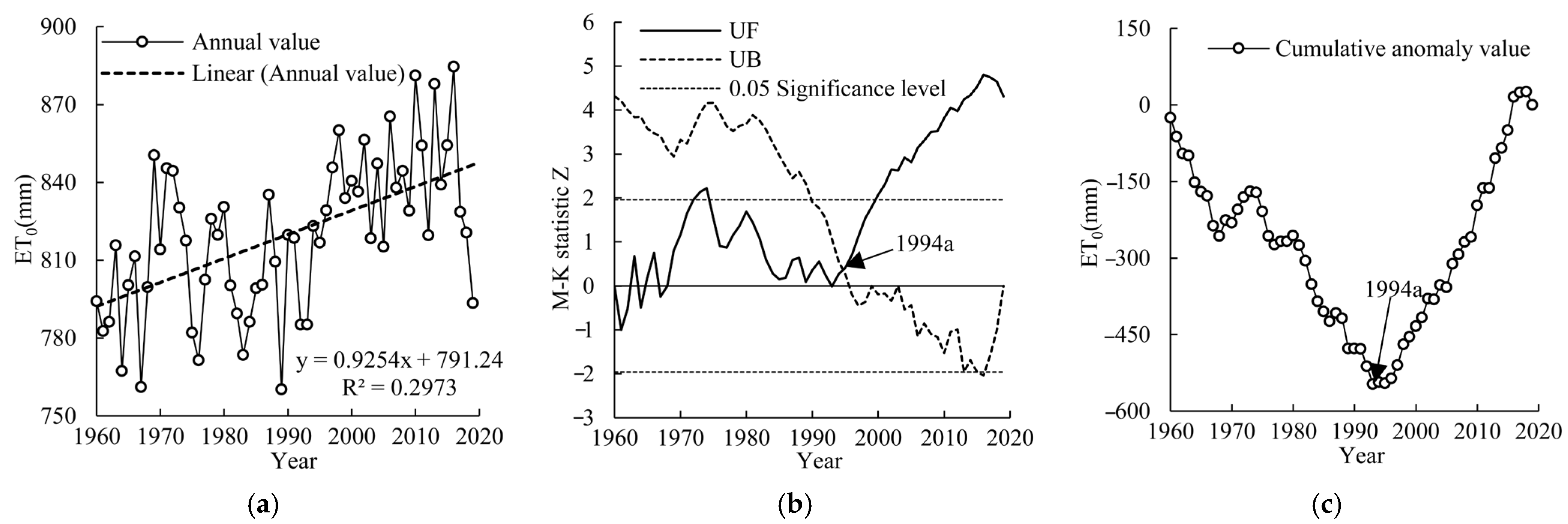
ET0 was calculated for each station based on meteorological data during 1960–2019 from 19 meteorological stations in and around the Taohe River basin. Site ET0 was weighted based on the Thiessen polygon to obtain the basin ET0 [48]. The interannual variation in the basin ET0 is shown in Figure 2a. The time series of ET0 showed a significant upward trend over 60 years, with a linear change rate of 0.93 mm/a, and the Mann–Kendall (M-K) statistic Z was 4.31, reaching a significance level of 0.05. The annual mean value of ET0 was 819.46 mm, and the coefficient of variation was 3.59%. The maximum value during 1960–2019 was 884.52 mm in 2016, the minimum value during 1960–2019 was 760.15 mm in 1989, and the extreme value ratio was 1.16. The M-K test is shown in Figure 2b. The ET0 time series jumped in 1994, which is consistent with the cumulative anomaly curve shown in Figure 2c. ET0 decreased from 1960 to 1993 and increased from 1994 to 2019, when the mean value of ET0 increased from 803.39 to 840.49 mm, with an increase of 4.62%. The ET0 time series reached a significance level of 0.05 in 2000 and showed a significant increase.

3.1.2. Spatial Distribution of Average Annual Value and Annual Change Rate of ET0

Kriging spatial interpolation was carried out based on the annual ET0 for 60 years at 19 stations in and around the basin. The spatial distribution of the average annual value of ET0 is shown in Figure 3a. The range of the basin ET0 was 779.8–927.6 mm, and ET0 presents an increasing variation from upstream to downstream. The upper and middle reaches of the basin were low-value areas with ET0 ranging from 779.8 to 829.0 mm. The lower reaches were high-value areas with ET0 ranging from 829.0 to 927.6 mm. The difference in the spatial distribution of ET0 was affected by the regional geographic environment and climatic conditions. The basin spans three geomorphic units from the upper reaches to the lower reaches, namely, the plateau, alpine canyon area, and loess hilly area. The upper and middle reaches are cold and humid, while the lower reaches are warm and arid. The spatial distribution of the linear change rate in ET0 is shown in Figure 3b. The change rate in ET0 in the basin was between −0.48 and 2.95 mm/a. The change rate in the upstream and downstream was lower, which was between −0.48 and 1.20 mm/a. The change rate in the middle reaches was higher, which was between 1.20 and 2.95 mm/a. The ET0 at 14 stations (73.68%) was significantly increased (p < 0.05). ET0 at 5 stations (26.32%) was not significantly increased (p > 0.05), and they were distributed in areas with low change rates around the upstream and downstream basins, namely, Weiyuan Station, Linxia Station, Yongjing Station, Guanghe Station, and Henan Station. Therefore, ET0 in the whole basin increased significantly except for Guanghe station.

3.1.3. Spatial Distribution of ET0 over Four Seasons

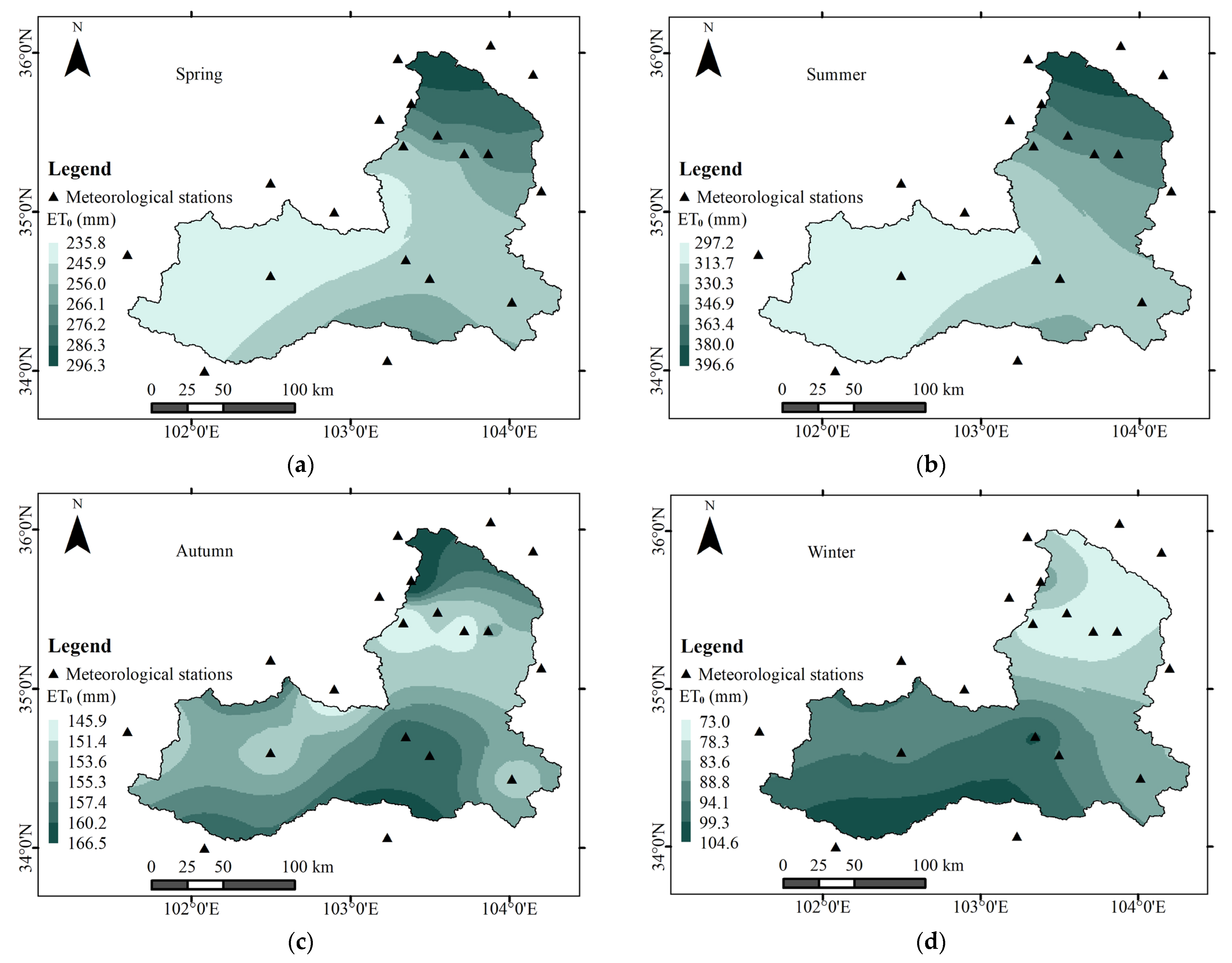
The average annual values from 19 stations during four seasons were used for spatial interpolation. The spatial distribution of the average annual values of ET0 for the four seasons is shown in Figure 4. The average annual values of ET0 in spring, summer, autumn, and winter were 251.93, 325.04, 153.92, and 88.51 mm, respectively. The order was summer, spring, autumn and winter, with the largest value in summer and the smallest value in winter, and the value in summer was 3.67 times that in winter. In both spring and summer, ET0 increased from the upper reaches to the lower reaches. The upper and middle reaches showed low values, ranging from 235.8 to 266.1 mm in spring and from 297.2 to 346.9 mm in summer, which increased by approximately 61.4 to 80.8 mm in summer compared with that in spring. The lower reaches showed high values, ranging from 266.1 to 296.3 mm in spring and from 346.9 to 396.6 mm in summer, which increased about 80.8~100.3 mm more in summer than in spring. In both autumn and winter, ET0 decreased from south to north, with high values in the upper and middle reaches and low values in the lower reaches, ranging from 145.9 to 166.5 mm in autumn and from 73.0 to 104.6 mm in winter, which decreased by approximately 61.9 to 72.9 mm in winter compared with that in autumn. In general, the distributions in autumn and winter were similar, with the upper and middle reaches showing greater values and the lower reaches showing lower values. Since ET0 in spring and summer accounted for 70.41% of the whole year, the spatial distribution of ET0 in spring and summer was similar to the distribution of annual ET0, with the upper and middle reaches showing lower values and the lower reaches showing larger values.

3.2. Variation Characteristics of Meteorological Factors Related to ET0

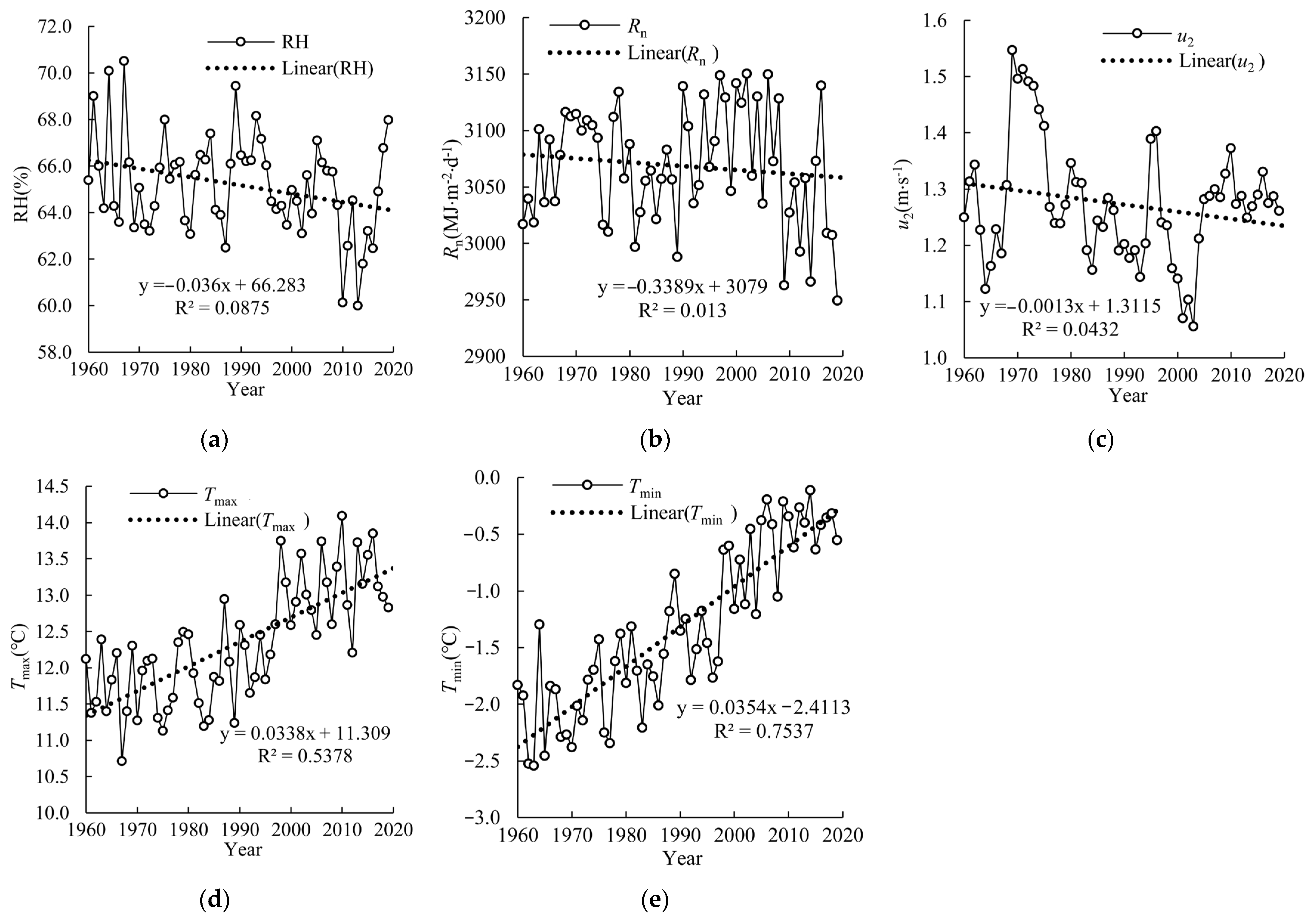
The FAO P-M model can be written as ET0 = f (Rn,u2,Tmax,Tmin,RH), where Rn, u2, Tmax, Tmin, and RH are the independent variables and ET0 is the dependent variable. Meteorological data from 1960 to 2019 from 19 meteorological stations and the FAO P-M formula were used to calculate Rn and u2. The basin Rn, u2, RH, Tmax, and Tmin were obtained by weighting the Thiessen polygon. The interannual variation trends in these five variables are shown in Figure 5. In Figure 5, linear regression was used to reveal variations in meteorological variables over time, identifying trends and linear change rates in meteorological data from 1960–2019. RH did not change significantly (Z = −1.57), with an annual mean value of 65.19%. Compared with the annual average value of 65.76% during 1960–1993 according to the period separation shown in Figure 2, RH decreased annually by 1.33% during 1994–2019 (64.43%). Rn did not change significantly (Z = −0.48), with an average annual value of 3068.66 MJ⋅m−2⋅d−1. Comparing the value of Rn during 1960–1993 (3066.80 MJ⋅m−2⋅d−1) with that during 1994–2019 (3071.08 MJ⋅m−2⋅d−1), Rn increased annually by 4.27 MJ⋅m−2⋅d−1 during 1960–2019. u2 did not change significantly (Z = −0.89), with an annual mean value of 1.27 m/s. Compared with the annual average value of 1.29 m/s during 1960–1993, u2 showed an annual decrease of 0.03 m/s during 1994–2019 (1.26 m/s). Tmax showed a significant upward trend (Z = 5.84), with an average annual value of 12.34 ℃, and the average annual value of Tmax during 1960–1993 (11.82 ℃) was 1.21 ℃ lower than that during 1994–2019 (13.03 ℃). Tmin showed a significant upward trend (Z = 7.65), with an annual average of −1.33 ℃. Compared with the annual average value of −1.82 ℃ during 1960–1993, Tmin during 1994–2019 (−0.70 ℃) increased by 1.12 ℃. In conclusion, RH, Rn, and u2 did not change significantly, while Tmax and Tmin showed a significant upward trend.

3.3. Qualitative Correlation Analysis between ET0 and Meteorological Variables

The FAO P-M model shows that ET0 is a function of Rn, u2, Tmax, Tmin, and RH, and there is a certain correlation between the variables Rn, u2, Tmax, Tmin, RH, and the dependent variable ET0. The correlation coefficient, grey correlation degree, regression relationship curve, and path analysis were used to study the correlation between ET0 and meteorological variables and to qualitatively reveal the statistical correlation degree between ET0 and Rn, u2, Tmax, Tmin, and RH.

3.3.1. Correlation Coefficient and Grey Correlation Degree between ET0 and Meteorological Variables

The monthly time series of ET0, Rn, u2, Tmax, Tmin, and RH were used to calculate the correlation coefficient and grey correlation degree between ET0 and each meteorological variable. ET0 and Rn are monthly values, and u2, Tmax, Tmin, and RH are monthly daily mean values. The calculation results are shown in Table 1. The order for the correlation coefficients between meteorological variables and ET0 is Rn, Tmax, Tmin, RH, u2, and the order for the grey correlation degree is Rn, Tmax, Tmin, u2, RH. ET0 had high consistency with the time series for Rn, Tmax, and Tmin, with Pearson’s coefficients of 0.989, 0.936, and 0.892; Spearman’s coefficients of 0.982, 0.941, and 0.890, and grey correlation degrees of 0.887, 0.804, and 0.736. Rn was strongly correlated with Tmax and Tmin, with Pearson’s coefficients of 0.901 and 0.869, and Spearman’s coefficients of 0.896 and 0.851, respectively. Tmax was strongly correlated with Tmin, with a Pearson’s coefficient of 0.977 and a Spearman’s coefficient of 0.974.

3.3.2. Regression Analysis between ET0 and Meteorological Variables

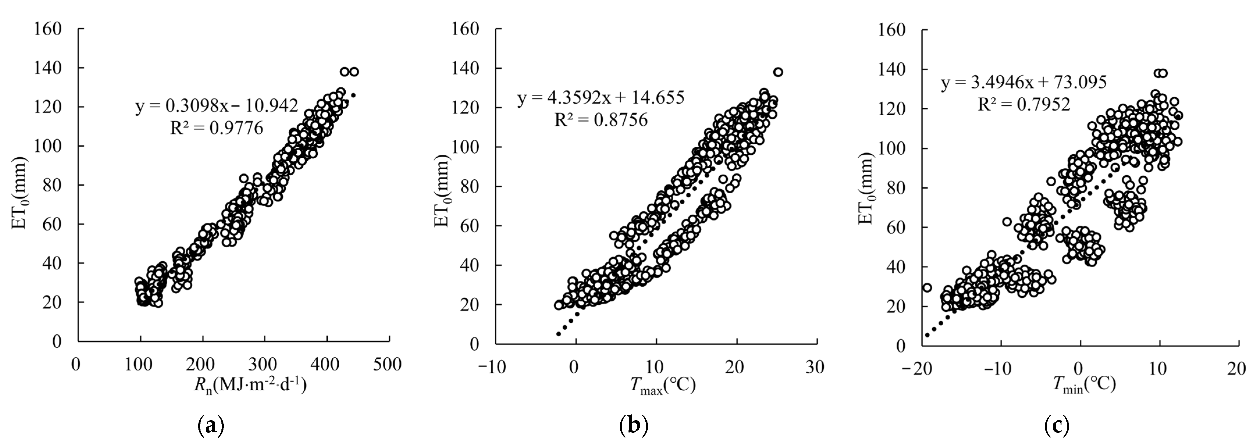
The regression curves between ET0 and Rn, u2, Tmax, Tmin, and RH are shown in Figure 6. In Figure 6, linear regression was used to reveal the correlation between ET0 and the meteorological variables. The more the data points are concentrated on a particular line and the closer R2 is to 1.0, the stronger the correlations between ET0 and the meteorological variables. ET0 is closely related to Rn, Tmax, and Tmin. The linear regression of ET0 and Rn is the most significant, and the determination coefficient R2 is 0.978 (Figure 6a). Second, the determination coefficients R2 between ET0 and Tmax and Tmin are 0.876 (Figure 6b) and 0.795 (Figure 6c), respectively. There is no obvious regression relationship between ET0 and RH or u2. The regression relationship between ET0 and various meteorological variables is consistent with the results of the correlation coefficient and grey correlation degree noted in Section 3.3.1, which shows that ET0 has a close statistical correlation with the time series for Rn, Tmax, and Tmin, and poor consistency with the time series for RH and u2.

3.3.3. Path Analysis of ET0 by Meteorological Variables

Path analysis was conducted on the five meteorological variables Rn, u2, Tmax, Tmin, and RH to determine the direct and indirect effects (effects through other factors) on ET0. The path analysis results are shown in Table 2. The path coefficient reflects the direct effect of various meteorological variables on ET0, and the order is Rn > Tmax > RH > u2 > Tmin. Rn has the largest direct effect, while Tmin has the smallest effect. The path coefficients of RH and u2 are negative, indicating that RH, u2, and ET0 change in opposite, while Rn, Tmax, Tmin, and ET0 change in the same direction. The indirect path coefficient reflects the indirect effect of each meteorological variable, and the order is Tmin > RH > Tmax > u2 > Rn. The indirect effect of Tmin is the largest, and the indirect effect of Rn is the smallest. The simple correlation coefficient comprehensively reflects the direct and indirect effects of each meteorological variable, and the order is Rn > Tmax > Tmin > RH > u2, which is the same as the calculation result for the Pearson’s coefficient. Rn is a meteorological variable closely related to the variation in ET0.

3.4. Quantitative Correlation Analysis between ET0 and Meteorological Variables

3.4.1. Sensitivity of ET0 to Variations in Meteorological Variables

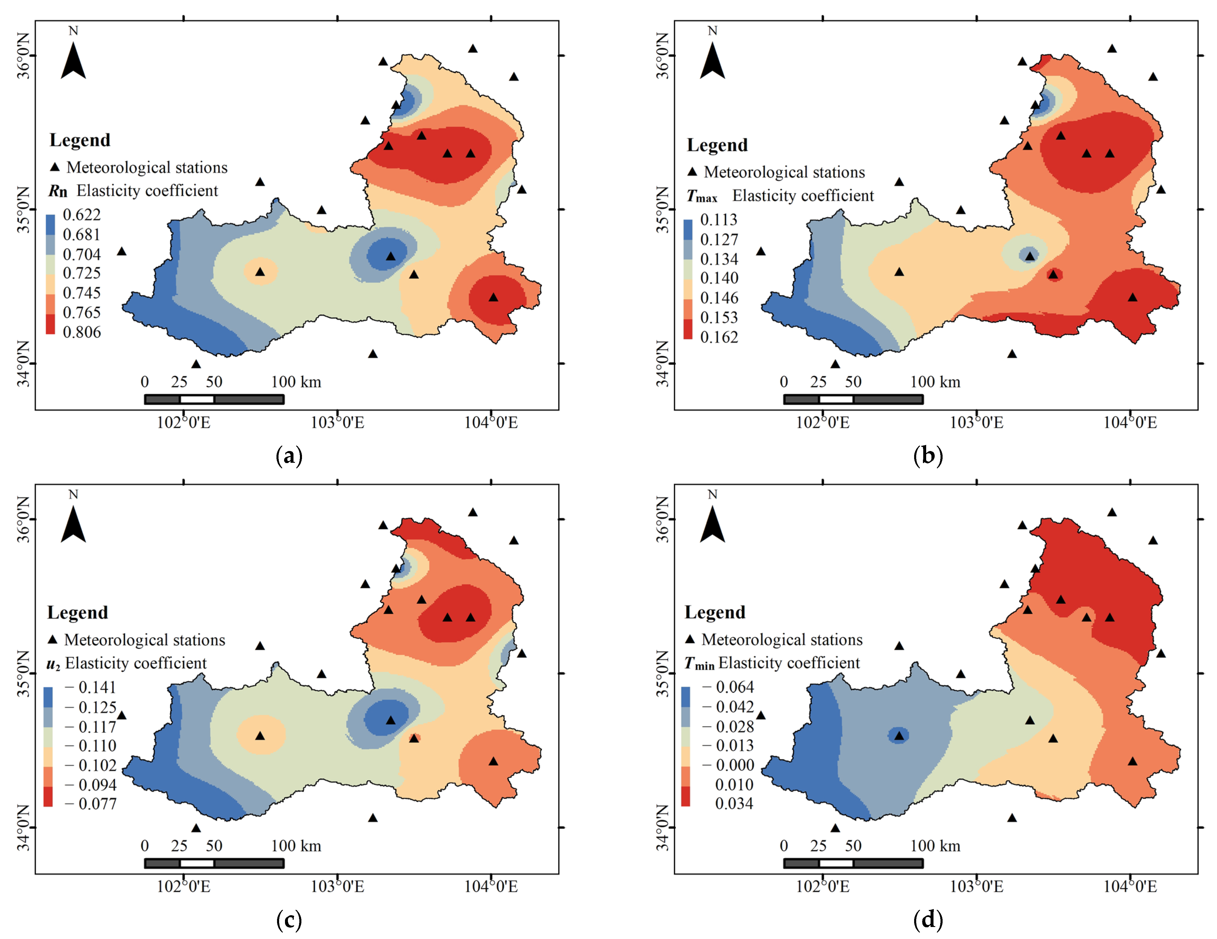
Based on the FAO P-M model, the elasticity coefficients for the five meteorological variables at 19 meteorological stations were obtained by solving differential equations (Equations (4)–(6)). The inverse distance weight method was used to carry out spatial interpolation with the elasticity coefficients for each meteorological variable. The spatial distribution of the Rn, u2, Tmax, Tmin, and RH elasticity coefficients is shown in Figure 7. The Rn (E-Rn) elasticity coefficient varies from 0.622 to 0.806, that is, if Rn increases by 10%, then ET0 increases by 6.22%~8.06%. E-Rn increases from upstream to downstream, and the high value area is located in the middle and lower reaches, with E-Rn 0.765~0.806. The Tmax (E-Tmax) elasticity coefficient varies from 0.113 to 0.162, that is, if Tmax increases by 10%, then ET0 increases by 1.13%~1.62%. The spatial distributions of E-Tmax and E-Rn are similar, and the high value range for E-Tmax and E-Rn is between 0.153 and 0.162. The u2 (E-u2) elasticity coefficient ranges from −0.141 to −0.077, that is, if u2 decreases by 10%, then ET0 increases by 0.77%~1.41%. The upper and middle reaches in the basin are high value areas, ranging from −0.141 to −0.125. The Tmin (E-Tmin) elasticity coefficient varies from −0.064 to 0.034, and ET0 varies from 0% to 0.64% if Tmin increases by 10%. The RH (E-RH) elasticity coefficient varies from −0.0015 to −0.0008, that is, if RH decreases by 10%, then ET0 increases by 0.008%~0.015%. The middle reaches in the basin are high value areas. In conclusion, the order in ET0 elasticity coefficients caused by variations in meteorological variables is Rn, Tmax, u2, Tmin, and RH. The Thiessen polygon weighted method was used to obtain the annual mean value for the basin. The maximum Rn elasticity coefficient was 0.722, followed by Tmax (0.143), u2 (−0.110), and Tmin (−0.016), and the minimum value for RH was −0.001. ET0 was the most sensitive to variations in Rn, followed by Tmax and u2. ET0 was least sensitive to variations in Tmin and RH.

3.4.2. Contribution Rate of Meteorological Variables to ET0 Variation

The contribution rate of meteorological variables to the variation in ET0 is shown in Table 3. The order for the contribution rate is Tmax > Tmin > u2 > Rn > RH. As the ET0 time series jumped in 1994, the period 1960–1993 is defined as the base period and the period 1994–2019 as the change period, which are shown in Figure 2b,c in Section 3.3.1. Compared with the base period (1960–1993), the average annual increase in ET0 was 37.10 mm during the change period (1994–2019). The contribution rates of each meteorological variable to the variation in ET0 were as follows: Tmax 11.49 mm (30.98%), Tmin 10.80 mm (29.11%), u2 2.44 mm (6.57%), Rn 0.82 mm (2.22%), and RH 0.02 mm (0.05%). Tmax is the most important meteorological variable that promotes the increase in ET0, followed by Tmin, u2, and Rn, and RH has the least influence. In the elasticity coefficient and contribution rate calculation, only RH, Rn, u2, Tmax, and Tmin were considered, and the contributions of mean temperature, altitude, and latitude were not considered. In the process of solving the differential equations for the elasticity coefficient, Rn was a compound variable deduced from Tmax and Tmin. As Rn was taken as an independent variable, the influence of Tmax and Tmin on Rn was not considered. The total contribution from the five variables was 68.93%.

4. Discussion

Qualitative and quantitative methods are combined in a progressive and complementary relationship. The linear trend method and the Mann–Kendall test were used to analyze trends in the time series for ET0 and meteorological variables. The Mann–Kendall test, Pettitt test, and cumulative anomaly curve were used to analyze the change points in the time series and the results were validated against each other to increase reliability. Correlation coefficients, grey correlation degree, regression curves, and pass analysis qualitatively revealed complex correlations between ET0 and meteorological variables. Differential solution equations for meteorological variables affecting ET0 were constructed on the basis of the FAO P-M model to identify the sensitivity of ET0 to variations in meteorological variables and the contribution from each meteorological variable. The exploratory application of multiple methods, with qualitative and quantitative methods complementing each other, provides new theoretical ideas and analytical bases to fully reveal the influencing mechanisms of ET0 variations.
ET0 in the Taohe basin showed a significant increase, with a linear change rate of 0.93 mm/a, and a sudden change occurring in 1994. The results are consistent with the previous research conclusion [32] that ET0 in the temperate continental zone and temperate monsoon zone of China showed an obvious upward trend from 1985 to 2015. The spatial distribution of ET0 ranged from 779.8 to 927.6 mm, increasing from upstream to downstream, with low values in the upper and middle reaches and high values in the lower reaches. It is consistent with the conclusion [28] that “ET0 gradually increases from upstream to downstream areas”. RH, Rn, and u2 did not change significantly, while Tmax and Tmin showed a significant increase. Fan et al. [32] found that the maximum and minimum temperatures have increased significantly during 1956 to 2015 in China, which is generally consistent with the conclusion of this study.
The regression relationship curve is consistent with the results for the correlation coefficient. ET0 is closely correlated with Rn, Tmax, and Tmin, but has poor consistency with the time series for RH and u2. ET0 was the most sensitive to variations in Rn, followed by Tmax and u2, and ET0 is the least sensitive to the variation in Tmin and RH. Yang et al. [28] showed that Rn was the most sensitive factor affecting ET0 in the Taohe River basin from 1981 to 2010, which is consistent with the conclusion of this study. Compared with the base period (1960–1993), the order for the contribution of meteorological variables to ET0 variation during the change period (1994–2019) was Tmax, Tmin, u2, Rn, and RH. Tmax was the most important meteorological variable (30.98%) that promoted an increase in ET0, followed by Tmin (29.11%), u2 (6.57%), and Rn (2.22%); RH (0.05%) had the least influence. This is consistent with the conclusion of previous studies that “the dominant factor is the increase in ET0 due to air temperature in the Taohe River basin from 1981 to 2010” [28]. Although ET0 is closely related to Rn and is most sensitive to variations in Rn, the contribution of Rn is only 2.22%, which is related to whether Rn has a significant magnitude of change from 1960 to 2019, based on Equation (9). The contribution is influenced by both the sensitivity coefficient and the magnitude of change in the meteorological variables. In the elasticity coefficient and contribution rate calculations, only RH, Rn, u2, Tmax, and Tmin were considered, and the contributions from other meteorological variables were not considered. Therefore, not all climatic and geographical environment conditions influencing ET0 variations have been taken into account and the total contribution from the above five variables was 68.93%.
Rn is a compound variable deduced from Tmax and Tmin, but it was taken as an independent variable in the process of solving the differential equations for the elasticity coefficient, which may affect the calculation results. The estimation of ET0 is available based on FAO P-M model on the basis of a large amount of meteorological data, but its implementation is still inconvenient due to its requirement for a large amount of meteorological data. Therefore, machine learning forecasting algorithms [33,49] for ET0 estimation are highly desirable.

5. Conclusions

Based on the FAO P-M model, we selected ET0 and five meteorological variables in the formula ET0 = f(Rn,u2,Tmax,Tmin,RH), and analyzed the spatiotemporal distribution of ET0 and meteorological variables. Qualitative and quantitative analysis methods were used to reveal the correlation between ET0 and various meteorological variables to clarify the sensitivity of ET0 to variations in meteorological variables and the contribution from each meteorological variable. The main conclusions are as follows:
(1)
ET0 in the Taohe basin showed a significant increase, with a linear change rate of 0.93 mm/a. The spatial distribution of ET0 ranged from 779.8 to 927.6 mm, increasing from upstream to downstream. The ET0 at 14 stations (73.68%) was significantly increased (p < 0.05), and that at 5 stations (26.32%) was not significantly increased (p > 0.05).
(2)
RH, Rn, and u2 did not change significantly, while Tmax and Tmin showed a significant increase. The annual average values of RH, Rn, u2, Tmax, and Tmin were 65.19%, 3068.66 MJ⋅m−2⋅d−1, 1.27 m/s, 12.34 °C, and −1.33 °C, while the annual average change was ﹣1.33%, + 4.27 MJ⋅m−2⋅d−1, −0.03 m/s, +1.21 °C, and +1.12 °C.
(3)
ET0 is closely correlated with Rn, Tmax, and Tmin, but has poor consistency with the time series for RH and u2. ET0 was the most sensitive to variations in Rn, followed by Tmax and u2, and ET0 is the least sensitive to the variation in Tmin and RH.
(4)
Compared with the base period (1960–1993), the order for the contribution of meteorological variables to ET0 increase during the change period (1994–2019) was Tmax (30.98%), followed by Tmin (29.11%), u2 (6.57%), and Rn (2.22%), and RH (0.05%), and the total contribution from these five variables was 68.93%.

Author Contributions

Data curation, Y.M. and D.S.; formal analysis, Y.M.; funding acquisition, Z.N. and D.S.; supervision, Y.M., Z.N., D.S., X.W. and L.J.; writing—original draft preparation, Y.M.; writing—review and editing, Z.N., X.W. and D.S. All authors have read and agreed to the published version of the manuscript.

Funding

This research was funded by the National Natural Science Foundation of China (NSFC) (Grant No. 42261003); the Innovation Fund of Higher Education of Gansu Province (Grant No. 2021B-120); the Special Project for the Construction of Scientific Research Team of the College of Water Conservancy and Hydropower Engineering, Gansu Agricultural University, China (Grant No. Gaucwky-04).

Data Availability Statement

Data are contained within the article.

Acknowledgments

The authors would like to thank all funds and laboratory facilities. We also gratefully acknowledge the anonymous reviewers for their constructive comments.

Conflicts of Interest

The authors declare no conflict of interest.

References

  1. Moran, M.S.; Rahman, A.F.; Washburne, J.C.; Goodrich, D.C.; Weltz, M.A.; Kustas, W.P. Combining the Penman-Monteith equation with measurements of surface temperature and reflectance to estimate evaporation rates of semiarid grassland. Agr. For. Meteorol. 1996, 80, 87–109. [Google Scholar] [CrossRef]
  2. Dinpashoh, Y.; Jahanbakhsh-Asl, S.; Rasouli, A.A.; Foroughi, M.; Singh, V.P. Impact of climate change on potential evapotranspiration (case study: West and NW of Iran). Theor. Appl. Climatol. 2019, 136, 185–201. [Google Scholar] [CrossRef]
  3. Xiong, Y.J.; Zhao, S.H.; Tian, F.; Qiu, G.Y. An evapotranspiration product for arid regions based on the three-temperature model and thermal remote sensing. J. Hydrol. 2015, 530, 392–404. [Google Scholar] [CrossRef]
  4. Adnan, S.; Ullah, K.; Khan, A.H.; Gao, S. Meteorological impacts on evapotranspiration in different climatic zones of Pakistan. J. Arid. Land. 2017, 9, 938–952. [Google Scholar] [CrossRef] [Green Version]
  5. Zhang, K.; Pan, S.; Zhang, W.; Xu, Y.; Cao, L.; Hao, Y.; Wang, Y. Influence of climate change on reference evapotranspiration and aridity index and their temporal-spatial variations in the Yellow River Basin, China, from 1961 to 2012. Quatern. Int. 2015, 380, 75–82. [Google Scholar] [CrossRef]
  6. Doorenbos, J. Guidelines for predicting crop water requirements. In Irrigation and Drainage Paper; FAO: Rome, Italy, 1977; Volume 24, pp. 1–179. [Google Scholar]
  7. Ma, N.; Szilagyi, J.; Jozsa, J. Benchmarking large-scale evapotranspiration estimates: A perspective from a calibration-free complementary relationship approach and FLUXCOM. J. Hydrol. 2020, 590, 125221. [Google Scholar] [CrossRef]
  8. Langensiepen, M.; Fuchs, M.; Bergamaschi, H.; Moreshet, S.; Cohen, Y.; Wolff, P.; Jutzi, S.C.; Cohen, S.; Rosa, L.M.G.; Li, Y.; et al. Quantifying the uncertainties of transpiration calculations with the Penman–Monteith equation under different climate and optimum water supply conditions. Agr. For. Meteorol. 2009, 149, 1063–1072. [Google Scholar] [CrossRef]
  9. Zeng, P.; Sun, F.; Liu, Y.; Che, Y. Future river basin health assessment through reliability-resilience-vulnerability: Thresholds of multiple dryness conditions. Sci. Total. Environ. 2020, 741, 140395. [Google Scholar] [CrossRef]
  10. Zeng, P.; Sun, F.; Liu, Y.; Wang, Y.; Li, G.; Che, Y. Mapping future droughts under global warming across China: A combined multi-timescale meteorological drought index and SOM-Kmeans approach. Weather Clim. Extrem. 2021, 31, 100304. [Google Scholar] [CrossRef]
  11. Lhomme, J.P. Towards a rational definition of potential evaporation. Hydrol. Earth Syst. Sci. 1997, 1, 257–264. [Google Scholar] [CrossRef] [Green Version]
  12. Zhu, B.; Zhang, Q.; Yang, J.; Li, C. Response of Potential Evapotranspiration to Warming and Wetting in Northwest China. Atmosphere 2022, 13, 353. [Google Scholar] [CrossRef]
  13. Irmak, S.; Kabenge, I.; Skaggs, K.E.; Mutiibwa, D. Trend and magnitude of changes in climate variables and reference evapotranspiration over 116-yr period in the Platte River Basin, central Nebraska—USA. J. Hydrol. 2012, 420, 228–244. [Google Scholar] [CrossRef]
  14. Sun, S.; Chen, H.; Wang, G.; Li, J.; Mu, M.; Yan, G.; Xu, B.; Huang, J.; Wang, J.; Zhang, F.; et al. Shift in potential evapotranspiration and its implications for dryness/wetness over Southwest China. J. Geophys. Res. Atmos. 2016, 121, 9342–9355. [Google Scholar] [CrossRef] [Green Version]
  15. Zeng, P.; Sun, F.; Liu, Y.; Feng, H.; Zhang, R.; Che, Y. Changes of potential evapotranspiration and its sensitivity across China under future climate scenarios. Atmos. Res. 2021, 261, 105763. [Google Scholar] [CrossRef]
  16. Zhang, Q.; Zhang, L.; Huang, J.; Zhang, L.; Wang, W.; Sha, S. Spatial distribution of surface energy fluxes over the Loess Plateau in China and its relationship with climate and the environment. Sci. China Earth Sci. 2014, 57, 2135–2147. [Google Scholar] [CrossRef]
  17. Yu, Z.; Zhou, W.; Zhang, X. An attribution analysis of changes in potential evapotranspiration in the Beijing-Tianjin-Hebei Region under climate change. J. Trop. Meteorol. 2019, 25, 82–91. [Google Scholar]
  18. Dong, Q.; Wang, W.; Shao, Q.; Xing, W.; Ding, Y.; Fu, J. The response of reference evapotranspiration to climate change in Xinjiang, China: Historical changes, driving forces, and future projections. Int. J. Climatol. 2020, 40, 235–254. [Google Scholar] [CrossRef]
  19. Lin, P.; He, Z.; Du, J.; Chen, L.; Zhu, X.; Li, J. Impacts of climate change on reference evapotranspiration in the Qilian Mountains of China: Historical trends and projected changes. Int. J. Climatol. 2018, 38, 2980–2993. [Google Scholar] [CrossRef]
  20. Peng, S.; Ding, Y.; Wen, Z.; Chen, Y.; Cao, Y.; Ren, J. Spatiotemporal change and trend analysis of potential evapotranspiration over the Loess Plateau of China during 2011–2100. Agr. For. Meteorol. 2017, 233, 183–194. [Google Scholar] [CrossRef] [Green Version]
  21. Jhajharia, D.; Dinpashoh, Y.; Kahya, E.; Singh, V.P.; Fakheri-Fard, A. Trends in reference evapotranspiration in the humid region of northeast India. Hydrol. Process. 2012, 26, 421–435. [Google Scholar] [CrossRef]
  22. Dinpashoh, Y.; Babamiri, O. Trends in reference crop evapotranspiration in Urmia Lake basin. Arab. J. Geosci. 2020, 13, 372. [Google Scholar] [CrossRef]
  23. Di Nunno, F.; Granata, F. Future trends of reference evapotranspiration in Sicily based on CORDEX data and Machine Learning algorithms. Agric. Water Manag. 2023, 280, 108232. [Google Scholar] [CrossRef]
  24. Jerin, J.N.; Islam, H.M.T.; Islam, A.R.M.T.; Shahid, S.; Hu, Z.; Badhan, M.A.; Chu, R.; Elbeltagi, A. Spatiotemporal trends in reference evapotranspiration and its driving factors in Bangladesh. Theor. Appl. Climatol. 2021, 144, 793–808. [Google Scholar] [CrossRef]
  25. Fu, J.; Gong, Y.; Zheng, W.; Zou, J.; Zhang, M.; Zhang, Z.; Qin, J.; Liu, J.; Quan, B. Spatial-temporal variations of terrestrial evapotranspiration across China from 2000 to 2019. Sci. Total. Environ. 2022, 825, 153951. [Google Scholar] [CrossRef] [PubMed]
  26. Jiang, S.; Liang, C.; Cui, N.; Zhao, L.; Du, T.; Hu, X.; Feng, Y.; Guan, J.; Feng, Y. Impacts of climatic variables on reference evapotranspiration during growing season in Southwest China. Agr. Water Manag. 2019, 216, 365–378. [Google Scholar] [CrossRef]
  27. Zhang, K.; Zhu, G.; Ma, J.; Yang, Y.; Shang, S.; Gu, C. Parameter analysis and estimates for the modis evapotranspiration algorithm and multiscale verification. Water Resour. Res. 2019, 55, 2211–2231. [Google Scholar] [CrossRef]
  28. Yang, L.; Feng, Q.; Li, C.; Si, J.; Wen, X.; Yin, Z. Detecting climate variability impacts on reference and actual evapotranspiration in the Taohe River Basin, NW China. Hydrol. Res. 2016, 48, 596–612. [Google Scholar] [CrossRef] [Green Version]
  29. Li, C.B.; Yang, L.S.; Yang, W.J.; Wang, S.B. Land use and land cover change in Taohe River Basin and its driving forces. Sci. Geogr. Sin. 2014, 34, 848–855. (In Chinese) [Google Scholar]
  30. Sun, L.; Wang, Y.; Zhang, J.; Yang, Q.; Bao, Z.; Guan, X.; Guan, T.; Chen, X.; Wang, G. Impact of environmental change on runoff in a transitional basin: Tao River Basin from the Tibetan Plateau to the Loess Plateau, China. Adv. Clim. Change Res. 2019, 10, 214–224. [Google Scholar] [CrossRef]
  31. Allen, R.G.; Pereira, L.S.; Raes, D.; Smith, M. Crop Evapotranspiration—Guidelines for Computing Crop Water Requirements—FAO Irrigation and Drainage Paper 56; FAO: Rome, Italy, 1998; Volume 300, p. D5109. [Google Scholar]
  32. Fan, J.; Wu, L.; Zhang, F.; Xiang, Y.; Zheng, J. Climate change effects on reference crop evapotranspiration across different climatic zones of China during 1956–2015. J. Hydrol. 2016, 542, 923–937. [Google Scholar] [CrossRef]
  33. Talebi, H.; Samadianfard, S.; Kamran, K.V. Investigating the roles of different extracted parameters from satellite images in improving the accuracy of daily reference evapotranspiration estimation. Appl. Water Sci. 2023, 13, 59. [Google Scholar] [CrossRef]
  34. Dinpashoh, Y.; Jhajharia, D.; Fakheri-Fard, A.; Singh, V.P.; Kahya, E. Trends in reference crop evapotranspiration over Iran. J. Hydrol. 2011, 399, 422–433. [Google Scholar] [CrossRef]
  35. Wang, Z.; Xie, P.; Lai, C.; Chen, X.; Wu, X.; Zeng, Z.; Li, J. Spatiotemporal variability of reference evapotranspiration and contributing climatic factors in China during 1961–2013. J. Hydrol. 2017, 544, 97–108. [Google Scholar] [CrossRef]
  36. Yin, Y.; Wu, S.; Chen, G.; Dai, E. Attribution analyses of potential evapotranspiration changes in China since the 1960s. Theor. Appl. Climatol. 2010, 101, 19–28. [Google Scholar] [CrossRef]
  37. Zhu, C.H. A further discussion on the Climatological Calculating Method of Total Radiation (II). Trans. Atmos. Sci. 1982, 2, 196–206. (In Chinese) [Google Scholar]
  38. Liu, J.; Zhang, Q.; Singh, V.P.; Shi, P. Contribution of multiple climatic variables and human activities to streamflow changes across China. J. Hydrol. 2017, 545, 145–162. [Google Scholar] [CrossRef] [Green Version]
  39. Schaake, J.C. From climate to flow. Clim. Chang. US Water Resour. 1990, 89, 177–206. [Google Scholar]
  40. Gemmer, M.; Jiang, T.; Su, B.; Kundzewicz, Z.W. Seasonal precipitation changes in the wet season and their influence on flood/drought hazards in the Yangtze River Basin, China. Quatern. Int. 2008, 186, 12–21. [Google Scholar] [CrossRef]
  41. Pettitt, A.N. A Non-Parametric Approach to the Change-Point Problem. J. R. Stat. Soc. Ser. C 1979, 28, 126–135. [Google Scholar] [CrossRef]
  42. Lyu, J.; Yin, S.; Sun, Y.; Wang, K.; Luo, P.; Meng, X. Flood Runoff Simulation under Changing Environment, Based on Multiple Satellite Data in the Jinghe River Basin of the Loess Plateau, China. Remote Sens. 2023, 15, 550. [Google Scholar] [CrossRef]
  43. Kendall, M.G. Rank Correlation Methods; Charles Griffin: London, UK, 1975. [Google Scholar]
  44. Pan, H.; You, X.; Liu, S.; Zhang, D. Pearson correlation coefficient-based pheromone refactoring mechanism for multi-colony ant colony optimization. Appl. Intell. 2021, 51, 752–774. [Google Scholar] [CrossRef]
  45. Xiao, C.; Ye, J.; Esteves, R.M.; Rong, C. Using Spearman's correlation coefficients for exploratory data analysis on big dataset. Concurr. Comput. Pract. Exp. 2016, 28, 3866–3878. [Google Scholar] [CrossRef]
  46. Xu, J.; Liu, Z.; Yin, L.; Liu, Y.; Tian, J.; Gu, Y.; Zheng, W.; Yang, B.; Liu, S. Grey Correlation Analysis of Haze Impact Factor PM2.5. Atmosphere 2021, 12, 1513. [Google Scholar] [CrossRef]
  47. Dewey, D.R.; Lu, K.H. A Correlation and Path-Coefficient Analysis of Components of Crested Wheatgrass Seed Production1. Agron. J. 1959, 51, 515–518. [Google Scholar] [CrossRef]
  48. Wu, L.; Zhou, H.; Li, J.; Li, K.; Sun, X.; Lu, S.; Li, L.; Zhu, T.; Guo, Q. Thiessen polygon analysis and spatial pattern evolution of Neolithic cultural sites (8.0–4.0 ka BP) in Huaibei Plain of Anhui, East China. Quatern. Int. 2019, 521, 75–84. [Google Scholar] [CrossRef]
  49. Yildirim, D.; Küçüktopcu, E.; Cemek, B.; Simsek, H. Comparison of machine learning techniques and spatial distribution of daily reference evapotranspiration in Türkiye. Appl. Water Sci. 2023, 13, 107. [Google Scholar] [CrossRef]
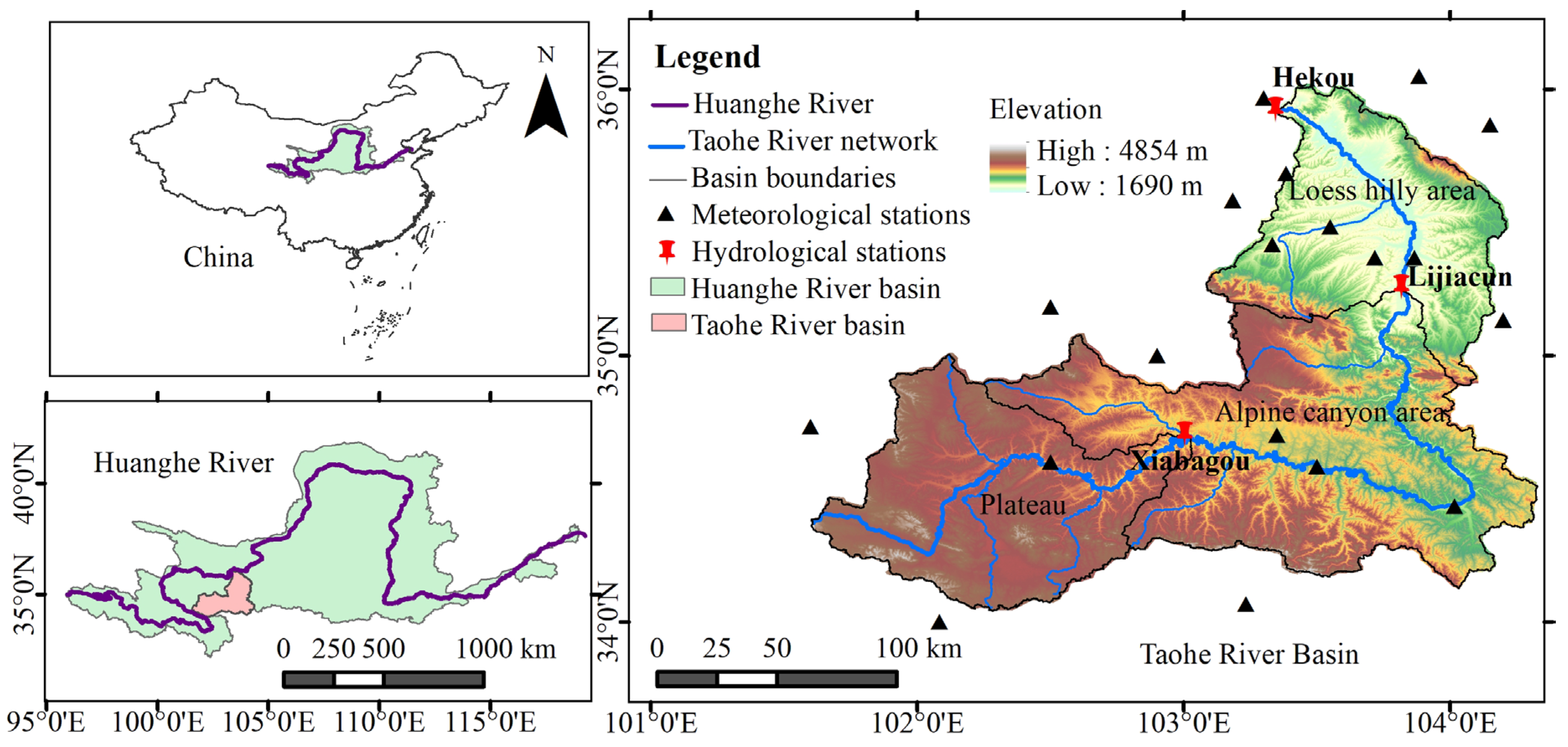
Figure 1. Geographical location and distribution of meteorological stations in the Taohe River basin.
Water 15 02264 g001
Figure 2. Variation trend and change point analysis of ET0 in the Taohe River basin. (a) Interannual trend in ET0: (b) M-K test analysis; (c) cumulative anomaly curve.
Water 15 02264 g002
Figure 3. Spatial distribution of annual value and linear change rate in ET0 in the Taohe River basin: (a) spatial distribution of annual ET0; (b) spatial distribution of linear change rate in ET0.
Water 15 02264 g003
Figure 4. Spatial distribution of ET0 annual value in four seasons in the Taohe River basin: (a) spring; (b) summer; (c) autumn; (d) winter.
Water 15 02264 g004
Figure 5. Interannual variation in meteorological variables: (a) RH; (b) Rn; (c) u2; (d) Tmax; (e) Tmin.
Water 15 02264 g005
Figure 6. Regression relationship between ET0 and meteorological variables: (a) Rn; (b) Tmax; (c) Tmin; (d) RH; (e) u2.
Water 15 02264 g006aWater 15 02264 g006b
Figure 7. Spatial distribution of elasticity coefficients for meteorological variables in the Taohe River basin: (a) Rn; (b) Tmax; (c) u2; (d) Tmin; (e) RH.
Water 15 02264 g007aWater 15 02264 g007b
Table 1. Correlation between ET0 and meteorological variables.
Correlation CoefficientPearsonSpearmanGrey Relational Degree
ET0RHRnTmaxTminu2ET0RHRnTmaxTminu2
ET010.490 **0.989 **0.936 **0.892 **0.447 **10.489 **0.982 **0.941 **0.890 **0.486 **1
RH 10.493 **0.671 **0.786 **−0.169 ** 10.490 **0.67 4 **0.788 **−0.171 **0.614
Rn 10.901 **0.869 **0.495 ** 10.896 **0.851 **0.499 **0.887
Tmax 10.977 **0.245 ** 10.974**0.247 **0.804
Tmin 10.211 ** 10.198 **0.736
u2 1 10.625
Note: ** 0.01 significant level.
Table 2. Path analysis of ET0 by meteorological factors.
Meteorological FactorsPath Coefficient
(Direct Effect)
Indirect Path Coefficient (Indirect Effect)Simple Correlation Coefficient
RnTmaxRHu2TminΣ
Rn0.743 0.311−0.057−0.0130.0050.2460.989
Tmax0.3450.670 −0.078−0.0060.0060.5910.936
RH−0.1160.3660.232 0.0040.0050.6070.490
u2−0.0260.3680.0840.020 0.0010.4730.447
Tmin0.0060.6460.337−0.091−0.005 0.8860.892
Notes: Rn, Tmax, RH, u2, and Tmin represent net radiation, daily maximum temperature, relative humidity, wind speed at 2 m, and daily minimum temperature, respectively.
Table 3. Contribution rate of meteorological variables to ET0.
Meteorological FactorsElasticity CoefficientAverage Annual ValueAverage Annual ChangeAnnual Change in ET0/mmContribution Rate/%
Rn0.7223068.66 MJ⋅m−2⋅d−14.27 MJ⋅m−2⋅d−10.822.22
Tmax0.14312.34 °C1.21 °C11.4930.98
Tmin−0.016−1.33 °C1.12 °C10.8029.11
u2−0.1101.27 m/s−0.03 m/s2.446.57
RH−0.00165.19%−1.33%0.020.05
ET0-819.46 mm37.10 mm--
Notes: Rn, Tmax, RH, u2, and Tmin represent net radiation, daily maximum temperature, relative humidity, wind speed at 2 m, and daily minimum temperature, respectively.
Disclaimer/Publisher’s Note: The statements, opinions and data contained in all publications are solely those of the individual author(s) and contributor(s) and not of MDPI and/or the editor(s). MDPI and/or the editor(s) disclaim responsibility for any injury to people or property resulting from any ideas, methods, instructions or products referred to in the content.