TreatEEM—A Software Tool for the Interpretation of Fluorescence Excitation-Emission Matrices (EEMs) of Dissolved Organic Matter in Natural Waters

Abstract

Fluorescence excitation-emission matrices (EEMs) are a useful tool in aquatic sciences for monitoring and studying the biogeochemistry of organic matter in natural waters and engineered systems. Yet, the interpretation of the wealth of information available in EEMs requires the use of appropriate software. Existing software tools for the analysis of EEMs, offered by instrument producers, have limited treatment capabilities, while other freely available tools are based on the MATLAB or R programming languages, which require a certain level of programming skills and a pre-installation of MATLAB or R. Here, we present TreatEEM, the first non-commercial, stand-alone Windows-based software tool that provides comprehensive treatment of EEMs. Its greatest advantage is its user-friendly and interactive graphical user interface, providing a convivial and responsive graphical feedback on any action performed on either a single spectrum (recorded at one excitation wavelength) or EEM. The capabilities of TreatEEM, including (a) basic EEM treatment, such as simple inner filter correction, scatter removal, blank subtraction, Raman normalisation, smoothing, drift alignment etc., (b) extraction of useful parameters for DOM characterisation (Coble peaks and fluorescence indices) and (c) preparation of data for PARAFAC analysis plus presentation/manipulation of obtained PARAFAC components, are described in detail, along with a basic theoretical background on these most commonly used treatment steps of EEMs.

1. Introduction

Fluorescence spectroscopy has been shown to be useful in a number of disciplines relevant to physical, chemical, biological and medical sciences. In the water sciences, it is used for monitoring and studying the dynamics of dissolved organic matter (DOM) [1,2,3,4,5]. The fraction of DOM capable of absorbing light at the UV and visible wavelengths is called chromophoric/coloured DOM (CDOM), whereas the fraction of CDOM that emits part of the absorbed light as fluorescence is called fluorescent DOM (FDOM). Even if the percentage of CDOM is very hard to estimate, it is proposed to range from 20% in open ocean to 70% in coastal regions where riverine DOM dominates [6]. Although it represents a small and not well-defined fraction of the entire DOM pool in the ocean, CDOM plays an important role in the carbon cycle, as well as in the cycling of trace elements and gases important to biological activity and global climate. CDOM is also of vital interest for aquatic ecosystem functioning by influencing the optical properties of seawater [6,7]. It mediates redox reactions of some trace metals such as Fe, which is biologically the most relevant trace metal, and influences the air–sea exchange of climate-relevant gases [8,9]. Furthermore, CDOM is an important class of compounds in wastewaters [10] and molecules of concern in drinking water, since they can form harmful by-products during the disinfection process [11].

With the development of modern spectrofluorometers, FDOM is mostly studied by using excitation-emission matrices (EEMs), where fluorescence peaks are attributed to groups of fluorophores with known excitation/emission maxima. The EEM is obtained by collecting the emission scans at a wide range of excitation wavelengths (typically from 200 to 500 nm) and arranging them in a matrix resulting in a contour graph of fluorescence intensity as a function of emission (λ_em) and excitation wavelengths (λ_ex).

In natural water sciences, EEMs can provide information on the main origin of DOM components and their biological lability, as well as on changes within the DOM pool resulting from different processes such as biological processes of production and degradation, photobleaching, humification or mixing of water mases [5,12,13,14,15,16,17]. In coastal waters, a decrease in fluorescence intensity and a hypsochromic shift in fluorescence maxima (shift to shorter wavelengths) is often observed in the seaward direction as a result of photobleaching [6]. Protein-like and pigment-like fluorophores have shown an evident relationship with elevated biological activity; they are therefore considered evidence for DOM production [6,18,19]. These components appear to be microbially degradable, whereas humic-like components appear to be photodegradable but resistant to microbial degradation [5,20,21]. Humic-like FDOM has therefore been widely used as a potential tracer of refractory DOM [22], which plays an important role in carbon storage in the sea.

Besides understanding the DOM biogeochemistry in natural waters, EEMs can provide a useful tool in other water applications such as (a) predicting the treatability and potential of disinfection by-products formation in drinking water [11,23], (b) tracing the leachate contamination of ground water [24], (c) identification of textile wastewater in water bodies [25], (d) monitoring of (i) wastewater [26], (ii) sewage treatment impacts on aquatic systems [10,27], (iii) fluorescent whitening agents as a marker of an anthropogenic pollution [28], and (e) tracking oil-related DOM after oil spills [3,29]. There are many other utilities of EEMs, e.g., determining the individual binding parameters of organic matter components with metals [30], assessing soil health [31], investigating the DOM formed during composting [32], and identifying the geographical origin of plants [33]; they can also have different uses in medicine [34,35,36,37].

Despite their potential, the information contained in the EEMs is very difficult to interpret. There are several software tools capable of analysing EEMs. The most known and used is “drEEM toolbox” [38] developed for the MATLAB environment. Other MATLAB-based tools are “progMEEF”, developed by a group at the University of Toulon [39], and “efc”, developed by China University of Geosciences (Beijing, China) (https://www.nomresearch.cn/efc/indexEN.html (accessed on 26 April 2023)). Other MATLAB-based tools for EEM treatment exist, such as “EEM_corr”, that offers scattering correction in fluorescence data through an easily managed and freely available graphical user interface [40] or the EEMizer algorithm that automates the PARAFAC model building [41]. Recently an R-based program “staRdom” [42] was presented, allowing the treatment of both UV-Vis and fluorescence spectra. Philippe Massicotte provides his version of an R-based tool, named “eemR” (https://github.com/PMassicotte/eemR (accessed on 26 April 2023)). The programs provided by the instrument’s producers are mostly used to carry out measurements of samples, and they usually have limited treatment capabilities. The above-mentioned software tools require installation of either MATLAB (or MATLAB Runtime Library) or R software environment for statistical computing and graphics. To the best of our knowledge, no standalone windows-based software exists for such purposes. We think this is mostly because the various mathematical algorithms for the treatment of data already exist for MATLAB or R software environments, which simplifies the development of the specific software tools. To fill this gap, we present a free, windows-based software tool, TreatEEM. It is a user-friendly software developed for the visualisation and treatment of EEMs that does not require any other supporting program to be installed and run; it is therefore available to everyone and very easy to be used. Capabilities of TreatEEM are described along with the basic theoretical background related to the most common analysis of EEMs.

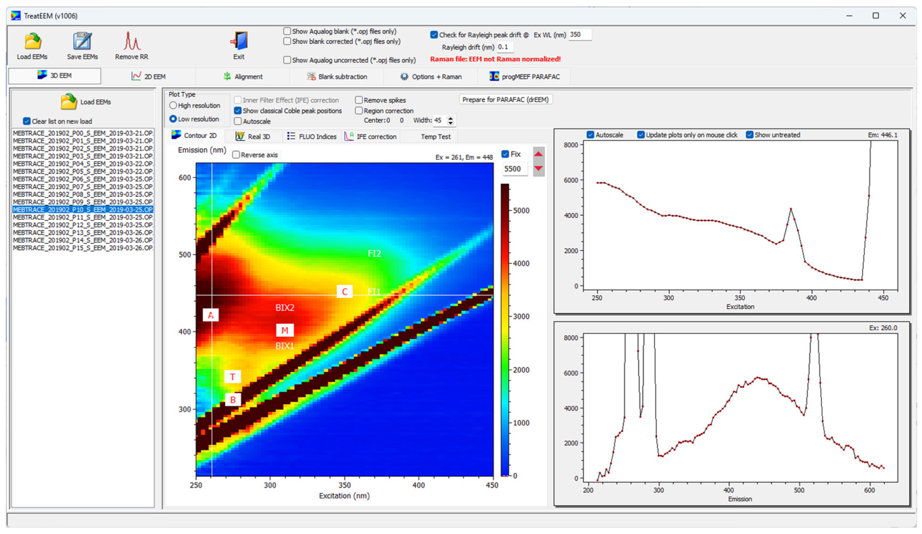
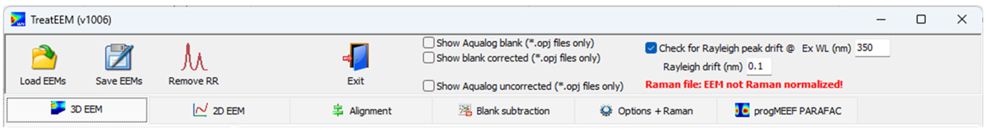
2. Basic Software Description and Main Graphical User Interface

TreatEEM was developed as a tool for visualisation and analysis of FDOM EEMs recorded by various producers of spectrofluorometers: Horiba, Shimadzu, Cary, Hitachi, Jasco. Various file types can be loaded (ASCII or binary); however, the actual version is tested using limited number of file types as provided by the software of these instrument producers. The most tested are Horiba Aqualog binary OPJ files. A partial structure of the binary OPJ file was reconstructed by reverse engineering (searching for specific segments within the binary file structure). Thus, errors when loading the file are possible, and users are invited to report the problem to the author of the program.

The greatest advantage and potential of the TreatEEM tool, if compared to other similar software tools, is its graphical user-friendly interface (GUI) and accurate correction for Raman and Rayleigh scattering. TreatEEM is fully interactive, and it provides a responsive graphical representation of the performed actions (Figure 1). EEMs can be visualised using both 2D contour and real 3D plots. Each separate spectrum can be presented using classical 2D plots. Numerous options to copy numerical data or graphics are incorporated. It is designed to allow users to follow the logical sequence of EEM treatment. It is assumed that users are familiar with the basic principles of the applied methodologies.

The following treatment routines for the analysis of EEMs are incorporated in TreatEEM:

• Inner filter effect (IFE) correction;
• Raman/Rayleigh (RR) scatter removal;
• Reconstruction of spectra under Raman/Rayleigh bands (interpolation);
• Blank subtraction;
• Raman normalisation;
• Alignment of drifted EEMs;
• Calculation of EEM wavelength drift;
• Manual correction of region inside of EEM;
• Smoothing;
• Resampling—EEM resolution increase;
• Selection of active EEM wavelength ranges;
• Peak picking;
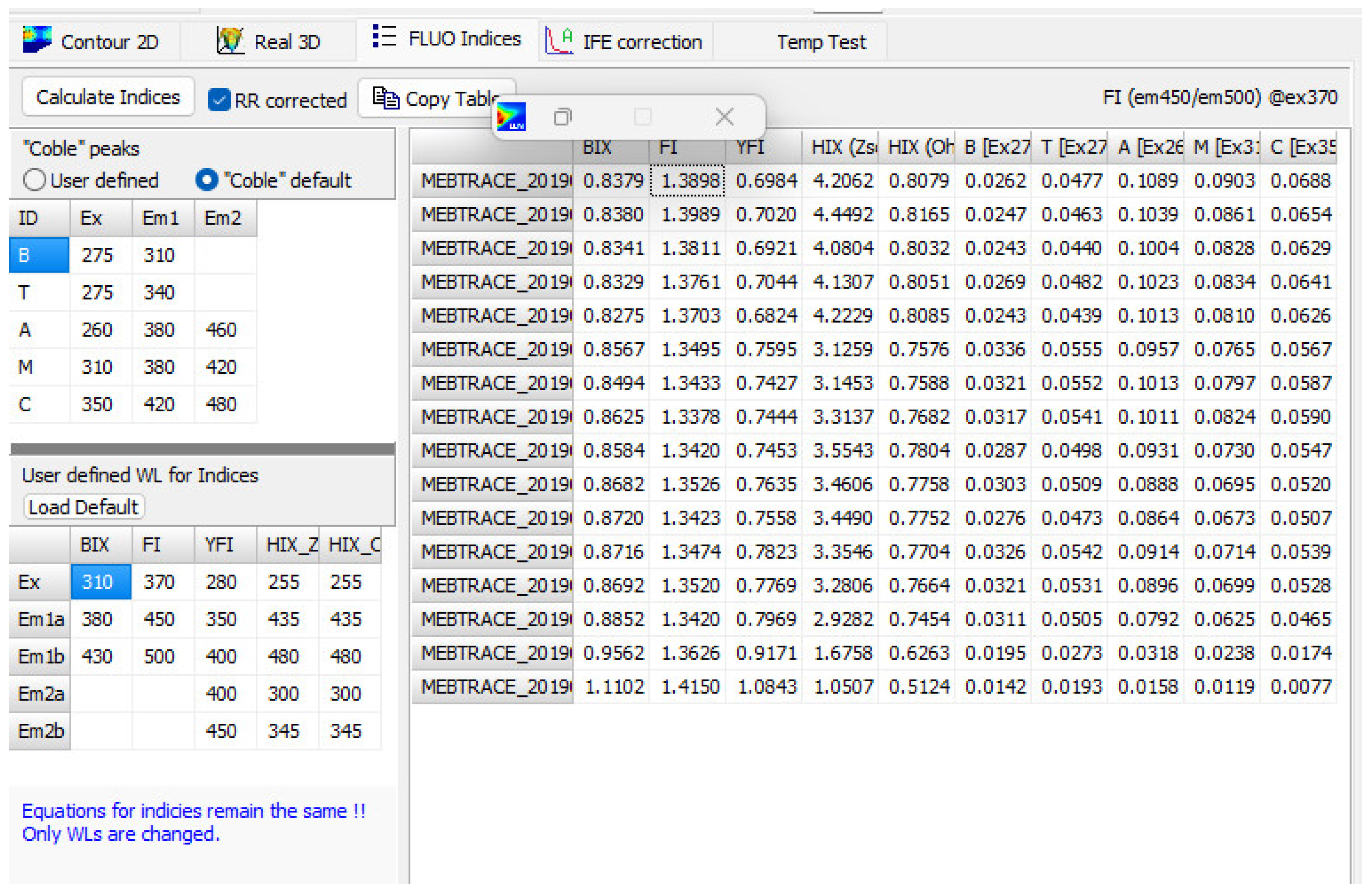
• Fluorescence indices (HIX, BIX, FI, YFI, Coble peaks);
• User-defined fluorescence indices;
• Preparation of data for PARAFAC analysis;
• Presentation of PARAFAC components;
• Reconstruction of EEMs using PARAFAC components.

The study of DOM often includes analysis of CDOM using UV-Vis spectrometry, along with the analysis of EEMs. Although the analysis of UV-Vis spectra and EEMs are often a part of the same software tools (e.g., “staRdom” [42]), we did not include the other functions inside of the TreatEEM as we developed a separate software dedicated only to the advanced analysis of UV-Vis spectra, called ASFit [43].

The top toolbar of the TreatEEM contains basic commands for opening the EEMs, saving the treated EEMs and activating the window for RR band removal (Figure 2). In case of Horiba OPJ files, there are a few additional options for the elaboration of EEMs contained in the OPJ file. If “Check for Rayleigh peak drift” is selected, the program will calculate the drift of the fluorescence spectra for the selected excitation wavelength (350 nm default). The calculation of the drift is based on the comparison of a theoretical position of the Rayleigh peak in single spectrum and the actual position determined by fitting the Rayleigh peak using the equation for Gaussian peak.

3. Initial EEM Treatment

3.1. Inner Filter Effect (IFE) Correction

A problem for practical EEM applications is the apparent non-multi-linearity of the fluorescence intensity resulting from sample absorption or sample scattering. The overall high sample absorption can lead to an IFE, at which the detected fluorescence signal can be misleading, limiting the linear dependence of fluorescence signals to low sample concentrations [44]. At high concentrations, the absorption of the intrinsic components of the sample can alter the detected signal by absorbing the excitation light through the sample, leading to non-uniform sample illumination (primary IFE), and by reabsorbing the emitted fluorescence (secondary IFE). To account for IFE correction, the set of absorbance files corresponding to each EEM file should be loaded. In the case of Horiba, the OPJ files already contain the UV-Vis spectra, recorded along with the fluorescence spectra. The IFE correction will be applied automatically for each file loaded by selecting the checkbox named “Inner Filter Effect (IFE) correction”. A simple and approximate method for IFE correction is based on the equation proposed by Lakowicz, 2006 [45]:

$$F_{\mathrm{A}}=F_1\times {10}^{(A_{\mathrm{ex}}+A_{\mathrm{em})}/2}$$

where F_A is the IFE-corrected fluorescence intensity, F₁ is the measured (uncorrected) fluorescence intensity, A_ex is the absorbance at the fluorescence excitation wavelength, and A_em is the absorbance at the selected fluorescence emission wavelength.

Note that the TreatEEM was conceived to deal with classical issues and hindrances of IFE that can be circumvented by a dilution (to a level of organic matter with absorbance lower than 0.7) instead of the IFE that can be generated by IFE-based fluorescent sensing systems [46]. For further reading about advanced IFE correction we refer the readers to Chen et al., 2018 [46] and Mazivila et al., 2022 [47].

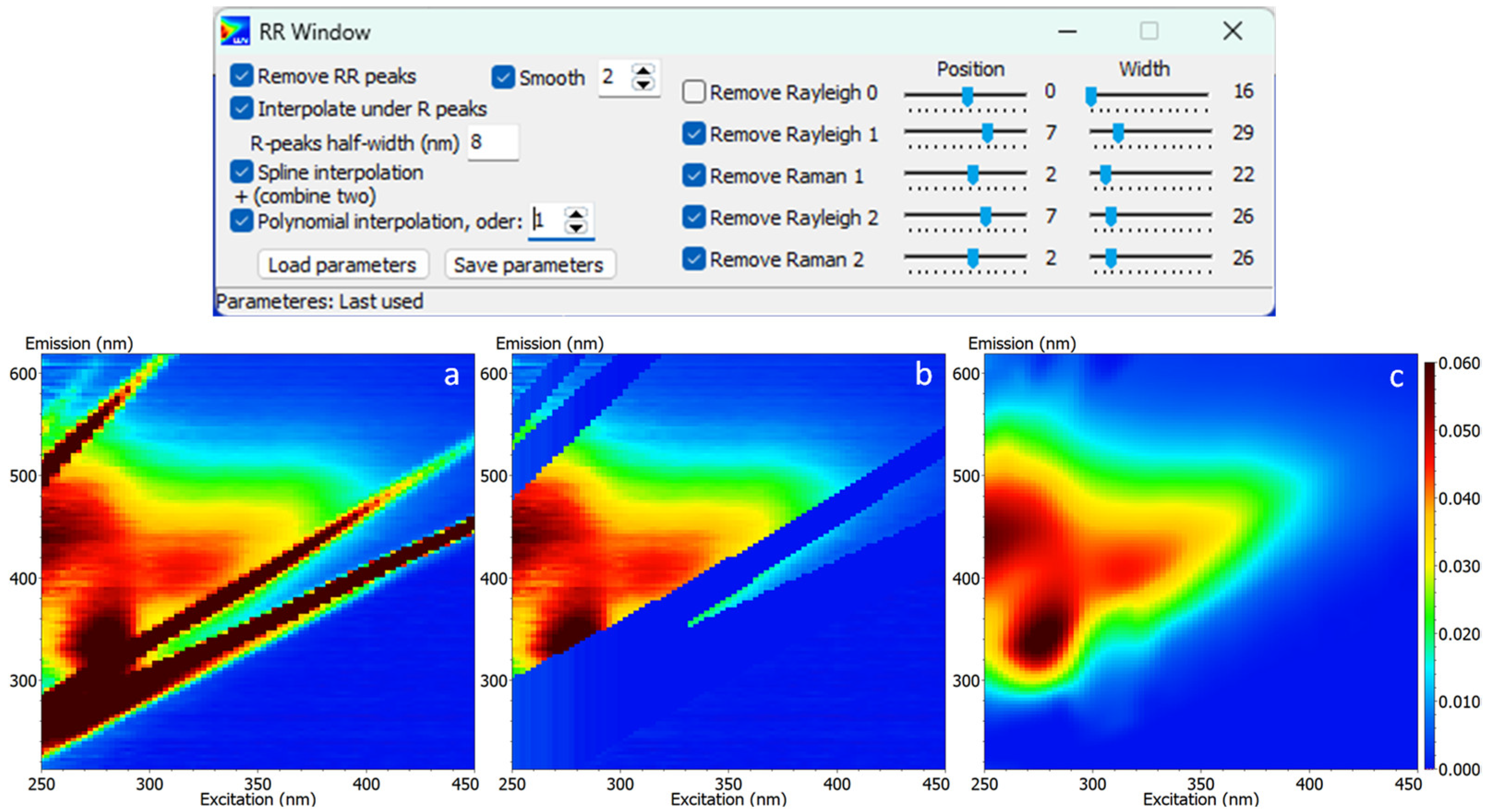
3.2. Raman and Rayleigh Scatter

Scattered light is another phenomenon that can create problems for quantitative analysis, especially for samples with low CDOM [48]. The most common types of scatters in EEMs are Rayleigh and Raman (RR). Rayleigh scattering is the scattered excitation light that peaks at the excitation wavelength equal to emission wavelength (1st band). Second-order Rayleigh band can be observed at an excitation wavelength that is half of the emission wavelength. Raman bands are the result of the inelastic scattering of the incoming light from water (or any other solvent) and peaks at a fixed emission/excitation wavelength pair.

The RR-scatter removal is performed in three main steps (Figure 3):

• Selection of bands to be removed by selecting corresponding checkboxes;
• Adjustment of the width of each scatter band;
• Interpolation of missing values under RR-bands.

The advantage of the provided procedure is that each change in the parameters is immediately visible on the EEM’s contour. It is recommended to apply smoothing of the spectra as the noise can cause a non-adequate interpolation. The interpolation of the missing parts of the spectrum, produced by scatter removal (replaced first by zeros), can be performed either by “spline”, “polynomial” or combined mathematical treatment. An additional algorithm is created to set a few non-zero values within the removed scatter points, with the purpose of helping the better interpolation using the above-mentioned mathematical treatments. It is advised that the blank EEM is subtracted before the scatter band removal, as this step could improve the shape of the spectra on both sides of the RR-bands, and it could also slightly narrow the width of the removal range. Once the set of parameters is adjusted, it can be saved for further use. The example, reported in Figure 3, clearly demonstrates the efficiency of the algorithms used for scatter band removal and interpolation. As the shape of the EEMs varies greatly depending on the sample source/matrix, the RR-removal process may provide a non-ideal treatment. The fine tuning of the algorithms behind the mathematical treatment is regularly improved to account for potential glitches of this type.

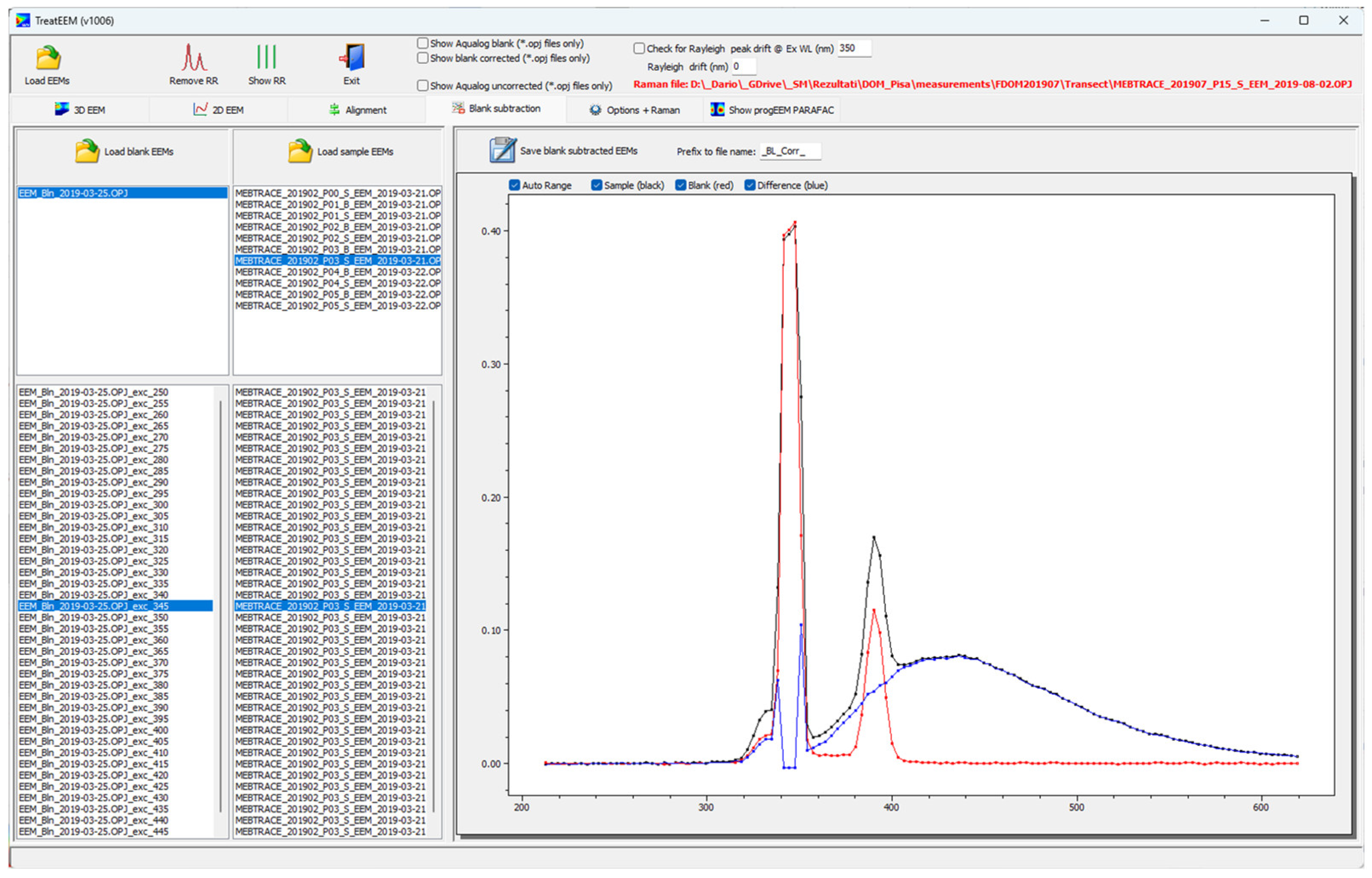
3.3. Blank Subtraction

The EEMs of ultrapure water are supposed to be free of any fluorescent peaks and are therefore used as blank. The usual practice is its recording for the inspection of the cleanliness of the system (especially cuvettes) and the partial removal of scattering bands by their subtraction from the EEM of the sample or to use for Raman normalisation [38]. In the TreatEEM, there are two options: (i) use a blank EEM for a selected set of sample EEMs, or (ii) use a different blank for each sample EEM (multiple pairs sample-blank). The effect of blank subtraction is visible for each excitation wavelength in the 2D plot (Figure 4). The blank-corrected EEMs can be saved by pressing the button “Save blank subtracted EEMs”. A user-defined prefix can be added to the blank-corrected files, which are stored in a separate folder named “_BL_Corrected”. In the case of Horiba OPJ files, the subtraction of blanks is possible by selecting the checkbox “Show blank corrected (*.opj files only)”. The blank corrected EEM is visible only in Contour 2D plot or Real 3D plot. It is mandatory that the matrix size of the blanks is the same as that of the samples. The subtracted data are saved in a form as currently displayed, e.g., Raman-normalised and/or resampled using option “Increase EEM resolution”.

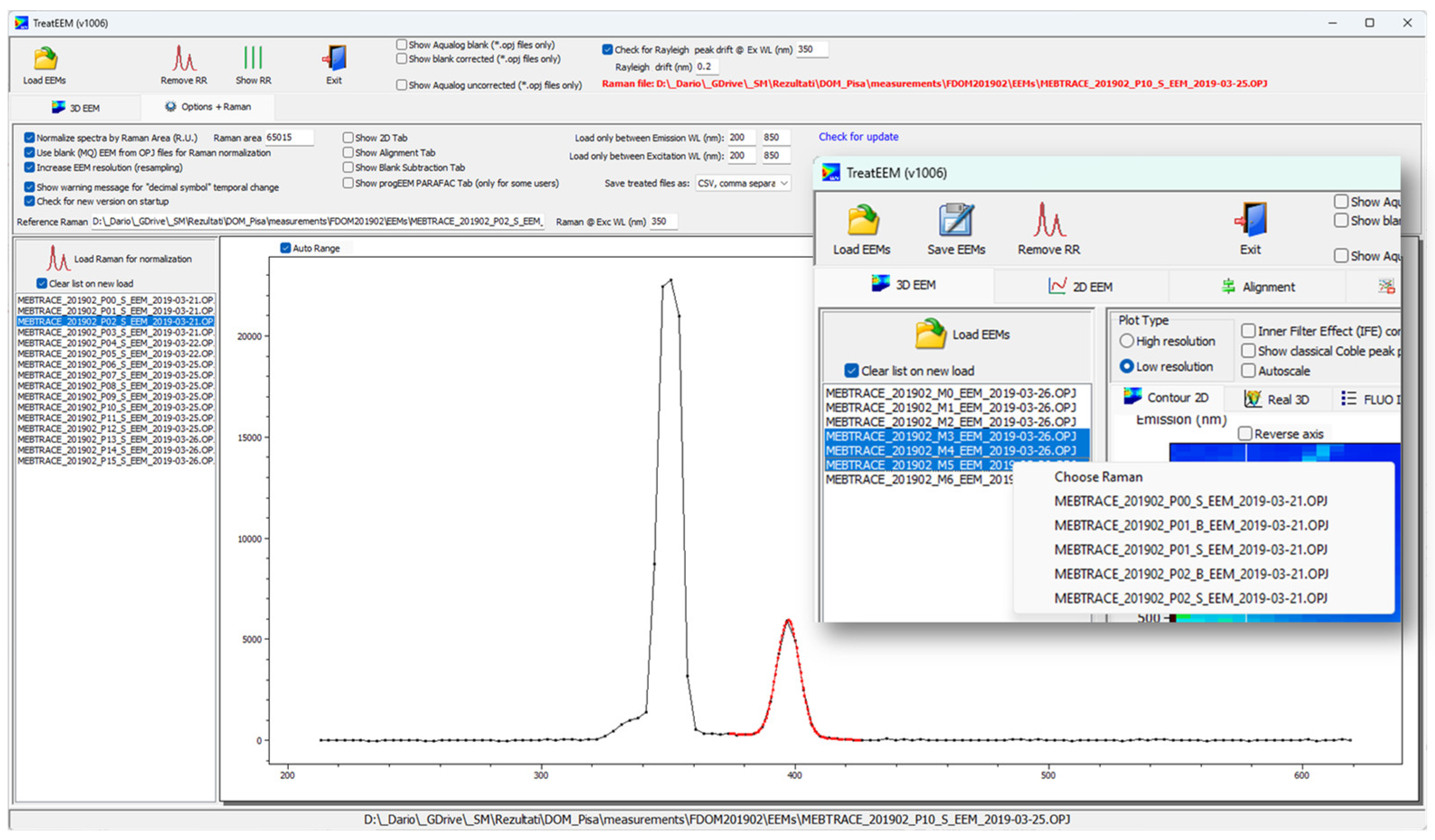
3.4. Raman Normalization

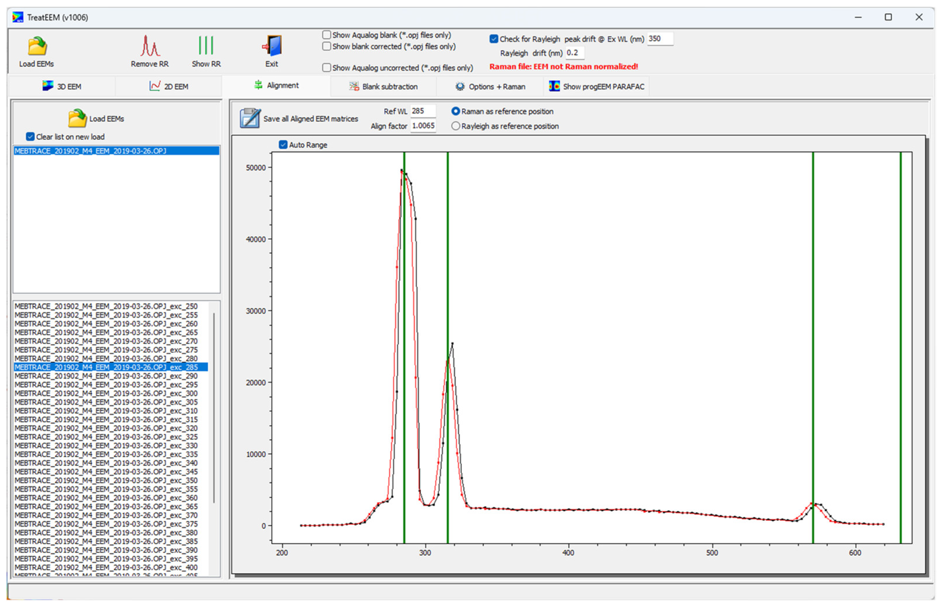
The fluorescence intensity can be expressed in arbitrary units, but it is subjected to changes due to changes in the intensity of the fluorescence source and the response of the detector; it is therefore necessary to calibrate the instrument with standardized samples in the same experimental conditions in order to enable the comparison of results among different studies and different instruments. Most often, this is accomplished by correcting the instrument intensity by using the Raman scattering of water at λ_ex = 350 nm and λ_em = 371–428 nm, i.e., expressing it in Raman units (R.U.). For this purpose, the area of the Raman peak in single emission spectra recorded at 350 nm excitation is used and fluorescence intensities are divided by the calculated peak area. In TreatEEM, the Raman peak recorded in ultrapure water at a selected excitation wavelength is fitted on a linear combination of Gaussian peak and first-order polynomial equations (Figure 5).

The polynomial equation is needed to account for a non-flat baseline under the Raman peak. The peak area is then computed by integrating only a fitted Gaussian peak. In this way, we do not needed to take care to centre and select the exact range for the peak integration, and the non-zero baseline is eliminated in the calculation. By default, λ_ex = 350 nm is used, but the user can manually set up another excitation wavelength. The fluorescence spectrum for a Raman correction can be separately recorded, or in the case of Horiba OPJ files, it can be taken from the blank file that is included in the OPJ file. In the case of separate Raman files that correspond to different sets of samples, all files should be loaded in the “Raman” file list. Thereafter, for a selected set of samples (“3D EEM” tab), a corresponding (correct) Raman file can be assigned from the dropdown menu (right-mouse click).

3.5. EEM Alignment

The positions of the Raman/Rayleigh bands in recorded EEMs could be shifted in either a positive or negative direction as a consequence of the instrument-specific influences. The extent of the drift is not the same for each excitation wavelength, and it is calculated as a factor that is the ratio of the observed and theoretically expected position of the Rayleigh or Raman peak in the single-emission spectra. This ratio is used to correct emission wavelength across the scanned emission wavelengths. The position of the Raman peak is calculated using the equation [49]:

$$Raman peak position \left({\lambda }_{\mathrm{ex}}\right)=1\times {10}^7{\left(\frac{1\times {10}^7}{{\lambda }_{\mathrm{ex}}}-3400\right)}^{-1}$$

The procedure includes the increase in the resolution of each spectrum by factor of 4 (linear interpolation) and the reconstruction of the drifted spectrum at the original emission wavelengths by a smoothed cubic spline function using the mathematical component provided by H. Lohninger (http://www.lohninger.com/helpcsuite/cubicspline.htm (accessed on 26 April 2023)). In this way, the original fluorescent peak intensities are preserved (Figure 6). Although the drift is usually at the level of a few nm, the alignment of spectra is suggested if the drift is higher than 5 nm in order to keep consistency with the correct positions of the characteristic fluorescence peaks recorded under different instrumental circumstances and/or to have a better comparison with the spectra of other authors.

4. Parameters Derived from EEMs

4.1. Peak Picking

Many studies investigate specific fluorescence peaks. They are commonly identified in aquatic FDOM and are often labelled with letters (A, C, M, B, T) according to Coble, 1996 [50]. The identification of these fluorescence peaks in EEMs is called ‘peak peaking’. Due to the difficulties in linking the fluorescence regions to the exact biochemical structure of the DOM, fluorophores generating them are categorized in groups named according to the fluorescence of standard substances e.g., humic-like and fulvic-like (according to International Humic Substances Society; IHSS standard samples) or protein-like (specifically tryptophan- or tyrosine-like). Common fluorescence components in aquatic DOM with designated letters by Coble, 2007 [6] are summarized in Table 1, including their fluorescence properties and potential sources.

Different peak intensity ratios can be used to gain information on DOM quality. For example, the ratio between tryptophan and humic-like substances (peak T/peak C) has been used to trace sewage contamination in riverine waters and estuaries, to detect contamination in recycled water systems and/or to estimate the DOM biodegradability [51,52,53]. The ratio between peaks A and T has been used to characterize the degree of anaerobic conversion of the organic matter during oil crop straw degradation [54].

Table 1. Common aquatic EEM peaks.

Component	Coble, 2007 [6]	λex,max/λem,max (nm)	Source
Humic-like	C	300–370/400–500	Terrestrial or anthropogenic; agriculture
Humic-like	A	237–260/400–500	Terrestrial or autochthonous
Marine humic-like	M	290–312/370–420	Anthropogenic; wastewater and agriculture
Protein-like Tyrosine-like	B	225–237/309–321 270–280/305–310	Autochthonous
Protein-like Tryptophan-like	T	225–237/340–381 270–280/340	Autochthonous
Pigment-like	P	400–430/660–670	Autochthonous
PAH-like [55]	-	220–280/311–350	Anthropogenic; oil-related or wildfires

Table 1. Common aquatic EEM peaks.

Component	Coble, 2007 [6]	λex,max/λem,max (nm)	Source
Humic-like	C	300–370/400–500	Terrestrial or anthropogenic; agriculture
Humic-like	A	237–260/400–500	Terrestrial or autochthonous
Marine humic-like	M	290–312/370–420	Anthropogenic; wastewater and agriculture
Protein-like Tyrosine-like	B	225–237/309–321 270–280/305–310	Autochthonous
Protein-like Tryptophan-like	T	225–237/340–381 270–280/340	Autochthonous
Pigment-like	P	400–430/660–670	Autochthonous
PAH-like [55]	-	220–280/311–350	Anthropogenic; oil-related or wildfires

4.2. Fluorescence Index

A common parameter in FDOM studies is the fluorescence index (FI), i.e., the ratio of emission intensity at specific emission/excitation wavelengths. The FI proposed to provide information about the source of FDOM is the ratio of emission intensity at 450 and 500 nm, excited at 370 nm [56]. The value of FI has been shown to be independent of the pH value and is ~1.4 for terrestrial sources and ~1.9 for autochthonous FDOM [56,57]. This corresponds to an increase in the emission maximum wavelengths with increasing biological activity.

The FI can be improved by using a wider fluorescence range formulated as Modified fluorescence index or Yeomin fluorescence index (YFI). The YFI is calculated as the average intensity over the 350–400 nm emission range divided by the average intensity over the 400–500 nm emission range, excited at 280 nm. Having a better resolution and less variation in different solutions, and being less sensitive to concentration-dependent effects than the FI, the YFI can help in differentiating the FDOM precursor materials [58,59]. As an example, in contrast to FI, YFI can distinguish between protein-like and amino-sugar-like standards [58]. Su et al., 2021 [54] successfully used YFI to track the evolution of the DOM during the anaerobic digestion of oil crop straw, and Derrien et al., 2019 [60] found it to be a reliable and robust index for tracking organic matter sources under early diagenetic processes.

4.3. Biological Activity and Humification Indices

In the literature, other fluorescence ratios have been reported to be related to DOM quality: the biological activity index (BIX) and humification index (HIX). BIX was proposed to investigate the contribution of biologically produced organic matter in a DOM pool [61,62]. It is defined as the ratio of the emission intensity at 380 and 430 nm upon excitation at 310 nm. The first emission wavelength corresponds to the intensity maximum of the fluorophore M (Table 1), whereas the second intensity maximum corresponds to the emission maximum of the fluorophore A (Table 1). In natural waters, BIX values higher than 1 indicate the presence of organic matter freshly produced by primary production, even if photochemical processes can also result in high BIX values [61]. In contrast, BIX values lower than 1 (0.6–0.7) are associated with a low biological production of DOM [62]. HIX, on the other hand, is taken from studies of organic matter in soil samples and is related to the degree of humification or aromaticity of fluorescent organics by quantifying the extent of the shifting of the emission spectra toward longer wavelengths with increasing humification. There are two ways for calculating this parameter, both included in the TreatEEM. Zsolnay et al., 1999 [63] first calculated HIX by dividing the emission intensity in the 435–480 nm range by the intensity in the 300–345 nm range, upon excitation at 255 nm. Ohno, 2002 [64] then corrected HIX for DOM concentration effects by defining it as the fluorescence intensity in the 300–345 nm region divided by the sum of intensity in the 300–345 nm and 435–480 nm regions. This correction is needed only for the samples with high absorbance (>0.3 cm⁻¹); however, the use of Ohno’s equation gives HIX values that are concentration independent, allowing for an easier comparison of results from different studies. HIX can be useful to study DOM in agricultural environments, e.g., for characterizing DOM in agricultural soils coming from different crop systems [65]. With increasing aromaticity degree, the emission at 255 nm shifts towards longer wavelengths, and HIX increases. In natural waters, this is often accompanied by a decrease in BIX. For example, in the eastern Indian Ocean, BIX decreased with depth together with protein peaks B and T [66], whereas HIX gradually increased with depth together with peaks A and C, indicating a higher concentration of humic-like fluorophores in deep waters as humic substances accumulate in the deep ocean with the aging of water masses [66]. In coastal waters, this pattern is evident when moving from open seawater to the land due to the input of humic-like fluorophores derived from terrestrial sources and sediment resuspension [67]. BIX and HIX also proved useful for studying wastewaters to evaluate the removal process of effluent DOM [68] and to identify the origin of some industrial effluents [53].

The peak piking method is implemented in TreatEEM in two ways. The first one is for a quick preview of the selected peak in the loaded set of EEMs, and it is performed by choosing the command “Plot fluorescence intensities at this WL” at the selected Ex/Em wavelengths using a right-mouse click. The program will plot the extracted fluorescence intensities, which can be copied in clipboard as a figure or numerical data set for transfer to other programs (Figure 7).

The second method corresponds to the determination of the classical Coble peaks along with the calculation of the above-described fluorescence indices (Figure 8). The Coble peaks are calculated using their default positions (but can be adjusted) and can be shown in the EEM by selecting the “Show classical Coble peaks positions” in the “Contour 2D” tab (see Figure 1). In the “FLUO Indices” tab, a user can define its own set of excitation and emission wavelengths for which the characteristic fluorescence peaks (as defined by the user) are extracted (user-defined setup is automatically saved for future use). Calculations of described indices can be performed in the same table. The equation for the calculation of selected indices is shown in the top-right position above the table (by clicking on the proper column in table). Note that the user can define the wavelengths for the indices, but the equations will remain the same. By double clicking on the selected column in the table, the numerical values will be plotted for a quick preview.

5. EEM Decomposition

Currently, the common practice is to mathematically resolve EEM datasets into underlying fluorescent components, which represent groups of fluorophores with similar fluorescence excitation–emission maxima, using parallel factor analysis (PARAFAC) [38]. PARAFAC provides estimates of the relative concentrations of each fluorescent component within samples. Fluorescence spectroscopy combined with PARAFAC has been applied to a variety of natural ecosystems, and it has also been used, albeit to a lesser extent, in engineered systems for monitoring water treatment [69,70]. PARAFAC analysis can provide a wealth of information about the dynamics of different components that are not otherwise apparent due to the overlapping of the spectra. It is generally supposed that similar underlying PARAFAC components can be attributed to similar DOM sources [69]. It is therefore particularly useful in studying ecosystems influenced by a variety of DOM sources, such as coastal waters where the marine DOM can be overshadowed by fluorophores originating from terrestrial sources [71,72]. The largest number of components (up to 12) was identified in studies that analysed a wide range of samples from lakes, streams, wetlands, estuaries, sea ice, waters influenced by anthropogenic activity, black-odour waterbodies, agricultural catchments, etc. [1,73,74,75,76,77,78].

As mentioned in the Introduction section, various and well-established software tools exists for PARAFAC analysis. The intention of TreatEEM is to prepare the set of EEMs that will be further used for PARAFAC analysis without the need for additional processing by these programs. Currently, the implemented procedure composes a set of files with a predefined structure for use in the drEEM toolbox. For the progMEEF software tool, there is no need for the specific structure of files/folders as there is for drEEM. The progMEEF tool reads ASCII-stored EEM files and performs PARAFAC analysis in which the file with the extracted components and their intensities in each EEM can be saved. This file can be used for the visualisation of the PARAFAC components in TreatEEM. Based on the selected number of components (component model 2C–6C), a reconstruction of each EEM is possible, along with the creation of residual EEM files if the “blank subtraction” procedure is combined.

The example reported in Figure 9 shows the excitation and emission spectra for a selected number of components (4C model in this case). The intensities of each PARAFAC component are displayed in the bottom graphs. It is also possible to compare the intensity of the same component (e.g., C1 in the first bottom graph) obtained with different models (indicated with different colours). TreatEEM also provides for the possibility to prepare the data file to be used in the OpenFluor database (“Save for OpenFluor” button). The option to copy the plot(s) or component intensities of one or all the components is offered in the drop-down menu (right-mouse click) (inset in Figure 9).

6. Conclusions

In this paper, we presented the first non-commercial, stand-alone Windows-based software tool that provides a comprehensive treatment of EEMs, called TreatEEM. The great advantage of TreatEEM and its main difference compared to other similar software tools is its independence, as it does not require any other supporting programs to be installed; other advantages include its user-friendly and interactive GUI and its ease of use. We have systematically described the capabilities of TreatEEM with its treatment routines for the analysis of EEMs, including preliminary EEM treatments, extraction of useful parameters for DOM characterization, and PARAFAC support. The description of the software was complemented by an elementary theoretical clarification of these most commonly used treatment steps of EEMs and parameters used for the analysis of DOM in both natural waters and engineered systems.

References

1. DeFrancesco, C.; Guéguen, C. Long-Term Trends in Dissolved Organic Matter Composition and Its Relation to Sea Ice in the Canada Basin, Arctic Ocean (2007–2017). J. Geophys. Res. Ocean. 2021, 126, e2020JC016578. [Google Scholar] [CrossRef]
2. Malakar, A.; Singh, R.; Westrop, J.; Weber, K.A.; Elofson, C.N.; Kumar, M.; Snow, D.D. Occurrence of Arsenite in Surface and Groundwater Associated with a Perennial Stream Located in Western Nebraska, USA. J. Hazard. Mater. 2021, 416, 126170. [Google Scholar] [CrossRef]
3. Baszanowska, E.; Otremba, Z. Fluorometric Detection of Oil Traces in a Seawater Column. Sensors 2022, 22, 2039. [Google Scholar] [CrossRef] [PubMed]
4. Park, J.; Kim, G.; Kwon, H.K.; Han, H.; Park, T.G.; Son, M. Origins and Characteristics of Dissolved Organic Matter Fueling Harmful Dinoflagellate Blooms Revealed by Δ13C and d/l-Amino Acid Compositions. Sci. Rep. 2022, 12, 15052. [Google Scholar] [CrossRef]
5. Bachi, G.; Morelli, E.; Gonnelli, M.; Balestra, C.; Casotti, R.; Evangelista, V.; Repeta, D.J.; Santinelli, C. Fluorescent Properties of Marine Phytoplankton Exudates and Lability to Marine Heterotrophic Prokaryotes Degradation. Limnol. Oceanogr. 2023, 68, 982–1000. [Google Scholar] [CrossRef]
6. Coble, P.G. Marine Optical Biogeochemistry: The Chemistry of Ocean Color. Chem. Rev. 2007, 107, 402–418. [Google Scholar] [CrossRef]
7. Stedmon, C.A.; Nelson, N.B. The Optical Properties of DOM in the Ocean. In Biogeochemistry of Marine Dissolved Organic Matter; Carlson, D.A., Hansell, C.A., Eds.; Academic Press: Cambridge, MA, USA, 2015; pp. 509–533. ISBN 0124071538, 9780124071537. [Google Scholar]
8. Pedrosa, P.; Souza, C.M.M.A.; Rezende, C.E. Linking Major Nutrients (C, H, N, and P) to Trace Metals (Fe, Mn, and Cu) in Lake Seston in Southern Brazil. Limnology 2007, 8, 233–242. [Google Scholar] [CrossRef]
9. Carpenter, L.J.; Nightingale, P.D. Chemistry and Release of Gases from the Surface Ocean. Chem. Rev. 2015, 115, 4015–4034. [Google Scholar] [CrossRef]
10. Baker, A. Fluorescence Excitation—Emission Matrix Characterization of Some Sewage-Impacted Rivers. Environ. Sci. Technol. 2001, 35, 948–953. [Google Scholar] [CrossRef]
11. Philibert, M.; Luo, S.; Moussanas, L.; Yuan, Q.; Filloux, E.; Zraick, F.; Murphy, K.R. Drinking Water Aromaticity and Treatability Is Predicted by Dissolved Organic Matter Fluorescence. Water Res. 2022, 220, 118592. [Google Scholar] [CrossRef] [PubMed]
12. Catalá, T.S.; Martínez-Pérez, A.M.; Nieto-Cid, M.; Álvarez, M.; Otero, J.; Emelianov, M.; Reche, I.; Arístegui, J.; Álvarez-Salgado, X.A. Dissolved Organic Matter (DOM) in the Open Mediterranean Sea. I. Basin–Wide Distribution and Drivers of Chromophoric DOM. Prog. Oceanogr. 2018, 165, 35–51. [Google Scholar] [CrossRef]
13. Retelletti Brogi, S.; Balestra, C.; Casotti, R.; Cossarini, G.; Galletti, Y.; Gonnelli, M.; Vestri, S.; Santinelli, C. Time Resolved Data Unveils the Complex DOM Dynamics in a Mediterranean River. Sci. Total Environ. 2020, 733, 139212. [Google Scholar] [CrossRef] [PubMed]
14. Galletti, Y.; Gonnelli, M.; Retelletti Brogi, S.; Vestri, S.; Santinelli, C. DOM Dynamics in Open Waters of the Mediterranean Sea: New Insights from Optical Properties. Deep Sea Res. Part I Oceanogr. Res. Pap. 2019, 144, 95–114. [Google Scholar] [CrossRef]
15. Zhou, Y.; Li, Y.; Yao, X.; Ding, W.; Zhang, Y.; Jeppesen, E.; Zhang, Y.; Podgorski, D.C.; Chen, C.; Ding, Y.; et al. Response of Chromophoric Dissolved Organic Matter Dynamics to Tidal Oscillations and Anthropogenic Disturbances in a Large Subtropical Estuary. Sci. Total Environ. 2019, 662, 769–778. [Google Scholar] [CrossRef]
16. Gómez-Letona, M.; Arístegui, J.; Hernández-Hernández, N.; Álvarez-Salgado, X.A.; Álvarez, M.; Delgadillo, E.; Pérez-Lorenzo, M.; Teira, E.; Hernández-León, S.; Sebastián, M. Deep Ocean Prokaryotes and Fluorescent Dissolved Organic Matter Reflect the History of the Water Masses across the Atlantic Ocean. Prog. Oceanogr. 2022, 205, 102819. [Google Scholar] [CrossRef]
17. Gonnelli, M.; Vestri, S.; Santinelli, C. Chromophoric Dissolved Organic Matter and Microbial Enzymatic Activity. A Biophysical Approach to Understand the Marine Carbon Cycle. Biophys. Chem. 2013, 182, 79–85. [Google Scholar] [CrossRef]
18. Yamashita, Y.; Tanoue, E. Chemical Characterization of Protein-like Fluorophores in DOM in Relation to Aromatic Amino Acids. Mar. Chem. 2003, 82, 255–271. [Google Scholar] [CrossRef]
19. He, Q.; Xiao, Q.; Fan, J.; Zhao, H.; Cao, M.; Zhang, C.; Jiang, Y. Excitation-Emission Matrix Fluorescence Spectra of Chromophoric Dissolved Organic Matter Reflected the Composition and Origination of Dissolved Organic Carbon in Lijiang River, Southwest China. J. Hydrol. 2021, 598, 126240. [Google Scholar] [CrossRef]
20. Catalá, T.S.; Mladenov, N.; Echevarría, F.; Reche, I. Positive Trends between Salinity and Chromophoric and Fluorescent Dissolved Organic Matter in a Seasonally Inverse Estuary. Estuar. Coast. Shelf Sci. 2013, 133, 206–216. [Google Scholar] [CrossRef]
21. Tong, G.; Yang, X.; Li, Y.; Jin, M.; Yu, X.; Huang, Y.; Zheng, R.; Wang, J.-J.; Chen, H. Impacts of Haze on the Photobleaching of Chromophoric Dissolved Organic Matter in Surface Water. Environ. Res. 2022, 212, 113305. [Google Scholar] [CrossRef] [PubMed]
22. Omori, Y.; Saeki, A.; Wada, S.; Inagaki, Y.; Hama, T. Experimental Analysis of Diurnal Variations in Humic-like Fluorescent Dissolved Organic Matter in Surface Seawater. Front. Mar. Sci. 2020, 7, 589064. [Google Scholar] [CrossRef]
23. Xu, X.; Kang, J.; Shen, J.; Zhao, S.; Wang, B.; Zhang, X.; Chen, Z. EEM–PARAFAC Characterization of Dissolved Organic Matter and Its Relationship with Disinfection by-Products Formation Potential in Drinking Water Sources of Northeastern China. Sci. Total Environ. 2021, 774, 145297. [Google Scholar] [CrossRef] [PubMed]
24. Baker, A.; Curry, M. Fluorescence of Leachates from Three Contrasting Landfills. Water Res. 2004, 38, 2605–2613. [Google Scholar] [CrossRef]
25. Liu, B.; Wu, J.; Cheng, C.; Tang, J.; Khan, M.F.S.; Shen, J. Identification of Textile Wastewater in Water Bodies by Fluorescence Excitation Emission Matrix-Parallel Factor Analysis and High-Performance Size Exclusion Chromatography. Chemosphere 2019, 216, 617–623. [Google Scholar] [CrossRef] [PubMed]
26. Carstea, E.M.; Bridgeman, J.; Baker, A.; Reynolds, D.M. Fluorescence Spectroscopy for Wastewater Monitoring: A Review. Water Res. 2016, 95, 205–219. [Google Scholar] [CrossRef] [PubMed]
27. Guo, W.; Xu, J.; Wang, J.; Wen, Y.; Zhuo, J.; Yan, Y. Characterization of Dissolved Organic Matter in Urban Sewage Using Excitation Emission Matrix Fluorescence Spectroscopy and Parallel Factor Analysis. J. Environ. Sci. 2010, 22, 1728–1734. [Google Scholar] [CrossRef] [Green Version]
28. Niloy, N.M.; Haque, M.M.; Tareq, S.M. Fluorescent Whitening Agents in Commercial Detergent: A Potential Marker of Emerging Anthropogenic Pollution in Freshwater of Bangladesh. Environ. Nanotechnol. Monit. Manag. 2021, 15, 100419. [Google Scholar] [CrossRef]
29. Bianchi, T.S.; Osburn, C.; Shields, M.R.; Yvon-Lewis, S.; Young, J.; Guo, L.; Zhou, Z. Deepwater Horizon Oil in Gulf of Mexico Waters after 2 Years: Transformation into the Dissolved Organic Matter Pool. Environ. Sci. Technol. 2014, 48, 9288–9297. [Google Scholar] [CrossRef]
30. Ohno, T.; Amirbahman, A.; Bro, R. Parallel Factor Analysis of Excitation–Emission Matrix Fluorescence Spectra of Water Soluble Soil Organic Matter as Basis for the Determination of Conditional Metal Binding Parameters. Environ. Sci. Technol. 2008, 42, 186–192. [Google Scholar] [CrossRef] [PubMed]
31. Rinot, O.; Borisover, M.; Levy, G.J.; Eshel, G. Fluorescence Spectroscopy: A Sensitive Tool for Identifying Land-Use and Climatic Region Effects on the Characteristics of Water-Extractable Soil Organic Matter. Ecol. Indic. 2021, 121, 107103. [Google Scholar] [CrossRef]
32. Yu, Z.; Liu, X.; Zhao, M.; Zhao, W.; Liu, J.; Tang, J.; Liao, H.; Chen, Z.; Zhou, S. Hyperthermophilic Composting Accelerates the Humification Process of Sewage Sludge: Molecular Characterization of Dissolved Organic Matter Using EEM–PARAFAC and Two-Dimensional Correlation Spectroscopy. Bioresour. Technol. 2019, 274, 198–206. [Google Scholar] [CrossRef]
33. Long, W.-J.; Wu, H.-L.; Wang, T.; Dong, M.-Y.; Chen, L.-Z.; Yu, R.-Q. Fast Identification of the Geographical Origin of Gastrodia Elata Using Excitation-Emission Matrix Fluorescence and Chemometric Methods. Spectrochim. Acta Part A Mol. Biomol. Spectrosc. 2021, 258, 119798. [Google Scholar] [CrossRef] [PubMed]
34. DaCosta, R.S.; Andersson, H.; Wilson, B.C. Molecular Fluorescence Excitation–Emission Matrices Relevant to Tissue Spectroscopy. Photochem. Photobiol. 2003, 78, 384. [Google Scholar] [CrossRef] [PubMed]
35. De Oliveira Neves, A.C.; Tauler, R.; de Lima, K.M.G. Area Correlation Constraint for the MCR−ALS Quantification of Cholesterol Using EEM Fluorescence Data: A New Approach. Anal. Chim. Acta 2016, 937, 21–28. [Google Scholar] [CrossRef] [PubMed]
36. Drezek, R.; Sokolov, K.; Utzinger, U.; Boiko, I.; Malpica, A.; Follen, M.; Richards-Kortum, R. Understanding the Contributions of NADH and Collagen to Cervical Tissue Fluorescence Spectra: Modeling, Measurements, and Implications. J. Biomed. Opt. 2001, 6, 385. [Google Scholar] [CrossRef] [PubMed]
37. Kang, S.; Josselin de Jong, E.; Higham, S.M.; Hope, C.K.; Kim, B. Fluorescence Fingerprints of Oral Bacteria. J. Biophotonics 2020, 13, e201900190. [Google Scholar] [CrossRef]
38. Murphy, K.R.; Stedmon, C.A.; Graeber, D.; Bro, R. Fluorescence Spectroscopy and Multi-Way Techniques. PARAFAC. Anal. Methods 2013, 5, 6557. [Google Scholar] [CrossRef] [Green Version]
39. Luciani, X.; Mounier, S.; Redon, R.; Bois, A. A Simple Correction Method of Inner Filter Effects Affecting FEEM and Its Application to the PARAFAC Decomposition. Chemom. Intell. Lab. Syst. 2009, 96, 227–238. [Google Scholar] [CrossRef] [Green Version]
40. Chiappini, F.A.; Alcaraz, M.R.; Goicoechea, H.C.; Olivieri, A.C. A Graphical User Interface as a New Tool for Scattering Correction in Fluorescence Data. Chemom. Intell. Lab. Syst. 2019, 193, 103810. [Google Scholar] [CrossRef]
41. Bro, R.; Vidal, M. EEMizer: Automated Modeling of Fluorescence EEM Data. Chemom. Intell. Lab. Syst. 2011, 106, 86–92. [Google Scholar] [CrossRef]
42. Pucher, M.; Wünsch, U.; Weigelhofer, G.; Murphy, K.; Hein, T.; Graeber, D. StaRdom: Versatile Software for Analyzing Spectroscopic Data of Dissolved Organic Matter in R. Water 2019, 11, 2366. [Google Scholar] [CrossRef] [Green Version]
43. Omanović, D.; Santinelli, C.; Marcinek, S.; Gonnelli, M. ASFit—An All-Inclusive Tool for Analysis of UV–Vis Spectra of Colored Dissolved Organic Matter (CDOM). Comput. Geosci. 2019, 133, 104334. [Google Scholar] [CrossRef]
44. Weitner, T.; Friganović, T.; Šakić, D. Inner Filter Effect Correction for Fluorescence Measurements in Microplates Using Variable Vertical Axis Focus. Anal. Chem. 2022, 94, 7107–7114. [Google Scholar] [CrossRef]
45. Lakowicz, J.R. (Ed.) Instrumentation for Fluorescence Spectroscopy. In Principles of Fluorescence Spectroscopy; Springer: Boston, MA, USA, 2006; pp. 27–61. ISBN 978-0-387-46312-4. [Google Scholar]
46. Chen, S.; Yu, Y.L.; Wang, J.H. Inner Filter Effect-Based Fluorescent Sensing Systems: A Review. Anal. Chim. Acta 2018, 999, 13–26. [Google Scholar] [CrossRef] [PubMed]
47. Mazivila, S.J.; Soares, J.X.; Santos, J.L.M. A Tutorial on Multi-Way Data Processing of Excitation-Emission Fluorescence Matrices Acquired from Semiconductor Quantum Dots Sensing Platforms. Anal. Chim. Acta 2022, 1211, 339216. [Google Scholar] [CrossRef]
48. Zepp, R.G.; Sheldon, W.M.; Moran, M.A. Dissolved Organic Fluorophores in Southeastern US Coastal Waters: Correction Method for Eliminating Rayleigh and Raman Scattering Peaks in Excitation-Emission Matrices. Mar. Chem. 2004, 89, 15–36. [Google Scholar] [CrossRef]
49. Lawaetz, A.J.; Stedmon, C.A. Fluorescence Intensity Calibration Using the Raman Scatter Peak of Water. Appl. Spectrosc. 2009, 63, 936–940. [Google Scholar] [CrossRef]
50. Coble, P.G. Characterization of Marine and Terrestrial DOM in Seawater Using Excitation-Emission Matrix Spectroscopy. Mar. Chem. 1996, 51, 325–346. [Google Scholar] [CrossRef]
51. Henderson, R.K.; Baker, A.; Murphy, K.R.; Hambly, A.; Stuetz, R.M.; Khan, S.J. Fluorescence as a Potential Monitoring Tool for Recycled Water Systems: A Review. Water Res. 2009, 43, 863–881. [Google Scholar] [CrossRef]
52. Qin, J.; Tan, J.; Zhou, X.; Yang, Y.; Qin, Y.; Wang, X.; Shi, S.; Xiao, K.; Wang, X. Measurement Report: Particle-Size-Dependent Fluorescence Properties of Water-Soluble Organic Compounds (WSOCs) and Their Atmospheric Implications for the Aging of WSOCs. Atmos. Chem. Phys. 2022, 22, 465–479. [Google Scholar] [CrossRef]
53. Rodríguez-Vidal, F.J.; García-valverde, M.; Ortega-azabache, B. Characterization of Urban and Industrial Wastewaters Using Excitation-Emission Matrix (EEM) Fluorescence: Searching for Specific Fingerprints. J. Environ. Manag. 2020, 263, 110396. [Google Scholar] [CrossRef] [PubMed]
54. Su, L.; Chen, M.; Wang, S.; Ji, R.; Liu, C.; Lu, X.; Zhen, G.; Zhang, L. Fluorescence Characteristics of Dissolved Organic Matter during Anaerobic Digestion of Oil Crop Straw Inoculated with Rumen Liquid. RSC Adv. 2021, 11, 14347–14356. [Google Scholar] [CrossRef]
55. Mendoza, W.G.; Riemer, D.D.; Zika, R.G. Application of Fluorescence and PARAFAC to Assess Vertical Distribution of Subsurface Hydrocarbons and Dispersant during the Deepwater Horizon Oil Spill. Environ. Sci. Process. Impacts 2013, 15, 1017. [Google Scholar] [CrossRef] [PubMed]
56. McKnight, D.M.; Boyer, E.W.; Westerhoff, P.K.; Doran, P.T.; Kulbe, T.; Andersen, D.T. Spectrofluorometric Characterization of Dissolved Organic Matter for Indication of Precursor Organic Material and Aromaticity. Limnol. Oceanogr. 2001, 46, 38–48. [Google Scholar] [CrossRef]
57. DePalma, S.G.S.; Arnold, W.R.; McGeer, J.C.; Dixon, D.G.; Smith, D.S. Variability in Dissolved Organic Matter Fluorescence and Reduced Sulfur Concentration in Coastal Marine and Estuarine Environments. Appl. Geochem. 2011, 26, 394–404. [Google Scholar] [CrossRef]
58. Heo, J.; Yoon, Y.; Kim, D.; Lee, H.; Lee, D. A New Fluorescence Index with a Fluorescence Excitation-Emission Matrix for Dissolved Organic. Desalination Water Treat. 2015, 57, 20270–20282. [Google Scholar] [CrossRef]
59. Kelso, J.E.; Baker, M.A. Organic Matter Is a Mixture of Terrestrial, Autochthonous, and Wastewater Effluent in an Urban River. Front. Environ. Sci. 2020, 7, 202. [Google Scholar] [CrossRef] [Green Version]
60. Derrien, M.; Shin, K.-H.; Hur, J. Assessment on Applicability of Common Source Tracking Tools for Particulate Organic Matter in Controlled End Member Mixing Experiments. Sci. Total Environ. 2019, 666, 187–196. [Google Scholar] [CrossRef]
61. Santos, L.; Pinto, A.; Filipe, O.; Cunha, Â.; Santos, E.B.H.; Almeida, A. Insights on the Optical Properties of Estuarine DOM—Hydrological and Biological Influences. PLoS ONE 2016, 11, e0154519. [Google Scholar] [CrossRef] [Green Version]
62. Huguet, A.; Vacher, L.; Relexans, S.; Saubusse, S.; Froidefond, J.M.; Parlanti, E. Properties of Fluorescent Dissolved Organic Matter in the Gironde Estuary. Org. Geochem. 2009, 40, 706–719. [Google Scholar] [CrossRef]
63. Zsolnay, A.; Baigar, E.; Jimenez, M.; Steinweg, B.; Saccomandi, F. Differentiating with Fluorescence Spectroscopy the Sources of Dissolved Organic Matter in Soils Subjected to Drying. Chemosphere 1999, 38, 45–50. [Google Scholar] [CrossRef] [PubMed]
64. Ohno, T. Fluorescence Inner-Filtering Correction for Determining the Humification Index of Dissolved Organic Matter. Environ. Sci. Technol. 2002, 36, 742–746. [Google Scholar] [CrossRef] [PubMed]
65. Gao, J.; Liang, C.; Shen, G.; Lv, J.; Wu, H. Spectral Characteristics of Dissolved Organic Matter in Various Agricultural Soils throughout China. Chemosphere 2017, 176, 108–116. [Google Scholar] [CrossRef] [PubMed] [Green Version]
66. Liu, Y.; Sun, J.; Wang, X.; Liu, X.; Wu, X.; Chen, Z.; Gu, T.; Wang, W.; Yu, L.; Guo, Y.; et al. Fluorescence Characteristics of Chromophoric Dissolved Organic Matter in the Eastern Indian Ocean: A Case Study of Three Subregions. Front. Mar. Sci. 2021, 8, 742595. [Google Scholar] [CrossRef]
67. Lei, J.; Yang, L.; Zhu, Z. Testing the Effects of Coastal Culture on Particulate Organic Matter Using Absorption and Fluorescence Spectroscopy. J. Clean. Prod. 2021, 325, 129203. [Google Scholar] [CrossRef]
68. Lyu, C.; Liu, R.; Li, X.; Song, Y.; Gao, H. Degradation of Dissolved Organic Matter in Effluent of Municipal Wastewater Plant by a Combined Tidal and Subsurface Flow Constructed Wetland. J. Environ. Sci. 2021, 106, 171–181. [Google Scholar] [CrossRef]
69. Ishii, S.K.L.; Boyer, T.H. Behavior of Reoccurring PARAFAC Components in Fluorescent Dissolved Organic Matter in Natural and Engineered Systems: A Critical Review. Environ. Sci. Technol. 2012, 46, 2006–2017. [Google Scholar] [CrossRef]
70. Murphy, K.R.; Hambly, A.; Singh, S.; Henderson, R.K.; Baker, A.; Stuetz, R.; Khan, S.J. Organic Matter Fluorescence in Municipal Water Recycling Schemes: Toward a Unified PARAFAC Model. Environ. Sci. Technol. 2011, 45, 2909–2916. [Google Scholar] [CrossRef]
71. Li, Y.; Song, G.; Massicotte, P.; Yang, F.; Li, R.; Xie, H. Distribution, Seasonality, and Fluxes of Dissolved Organic Matter in the Pearl River (Zhujiang) Estuary, China. Biogeosciences 2019, 16, 2751–2770. [Google Scholar] [CrossRef] [Green Version]
72. Marcinek, S.; Santinelli, C.; Cindrić, A.M.; Evangelista, V.; Gonnelli, M.; Layglon, N.; Mounier, S.; Lenoble, V.; Omanović, D. Dissolved Organic Matter Dynamics in the Pristine Krka River Estuary (Croatia). Mar. Chem. 2020, 225, 103848. [Google Scholar] [CrossRef]
73. Cory, R.M.; McKnight, D.M. Fluorescence Spectroscopy Reveals Ubiquitous Presence of Oxidized and Reduced Quinones in Dissolved Organic Matter. Environ. Sci. Technol. 2005, 39, 8142–8149. [Google Scholar] [CrossRef] [PubMed]
74. Asmala, E.; Haraguchi, L.; Markager, S.; Massicotte, P.; Riemann, B.; Staehr, P.A.; Carstensen, J. Eutrophication Leads to Accumulation of Recalcitrant Autochthonous Organic Matter in Coastal Environment. Global Biogeochem. Cycles 2018, 32, 1673–1687. [Google Scholar] [CrossRef]
75. Lu, K.; Gao, H.; Yu, H.; Liu, D.; Zhu, N.; Wan, K. Insight into Variations of DOM Fractions in Different Latitudinal Rural Black-Odor Waterbodies of Eastern China Using Fluorescence Spectroscopy Coupled with Structure Equation Model. Sci. Total Environ. 2022, 816, 151531. [Google Scholar] [CrossRef] [PubMed]
76. Eder, A.; Weigelhofer, G.; Pucher, M.; Tiefenbacher, A.; Strauss, P.; Brandl, M.; Blöschl, G. Pathways and Composition of Dissolved Organic Carbon in a Small Agricultural Catchment during Base Flow Conditions. Ecohydrol. Hydrobiol. 2022, 22, 96–112. [Google Scholar] [CrossRef]
77. Retelletti Brogi, S.; Cossarini, G.; Bachi, G.; Balestra, C.; Camatti, E.; Casotti, R.; Checcucci, G.; Colella, S.; Evangelista, V.; Falcini, F.; et al. Evidence of Covid-19 Lockdown Effects on Riverine Dissolved Organic Matter Dynamics Provides a Proof-of-Concept for Needed Regulations of Anthropogenic Emissions. Sci. Total Environ. 2022, 812, 152412. [Google Scholar] [CrossRef] [PubMed]
78. Zhuang, W.-E.; Chen, W.; Cheng, Q.; Yang, L. Assessing the Priming Effect of Dissolved Organic Matter from Typical Sources Using Fluorescence EEMs-PARAFAC. Chemosphere 2021, 264, 128600. [Google Scholar] [CrossRef] [PubMed]
Figure 1. Screenshot of the TreatEEM showing the graphical user interface (GUI).
Water 15 02214 g001
Figure 2. The main toolbar with commands for basic file handling.
Water 15 02214 g002
Figure 3. Main window for adjustment of parameters for Raman/Rayleigh scattering removal (top) and (a) uncorrected, (b) RR-removed and (c) interpolated contour EEM plots (bottom).
Water 15 02214 g003
Figure 4. Window showing a procedure of blank subtraction (colour codes: sample—black; blank—red; difference—blue).
Water 15 02214 g004
Figure 5. Raman peak fitting routine for calculation of its area (in red). Inset: an example of how to assign a specific Raman file to the set of sample EEMs.
Water 15 02214 g005
Figure 6. An example of spectrum alignment using Raman as a reference peak for excitation wavelength of 285 nm. Black — original spectrum; red — aligned spectrum. Green vertical lines represent the theoretical positions of Raman and Rayleigh peaks.
Water 15 02214 g006
Figure 7. An example of a quick preview pick picking result of loaded set of EEM files (x-axis represents the ordinal number of the EEMs).
Water 15 02214 g007
Figure 8. Screenshot of the program showing the calculation of fluorescence indices.
Water 15 02214 g008
Figure 9. Screenshot of the program showing the visualisation of PARAFAC components obtained using progMEEF software tool [39] (upper graphs; red lines are excitation spectra and blue lines are emission spectra) and their intensities in treated EEMs (bottom graphs; different colours show the same component but calculated with different component models: 2C–6C as indicated in the toolbar above).
Water 15 02214 g009
Disclaimer/Publisher’s Note: The statements, opinions and data contained in all publications are solely those of the individual author(s) and contributor(s) and not of MDPI and/or the editor(s). MDPI and/or the editor(s) disclaim responsibility for any injury to people or property resulting from any ideas, methods, instructions or products referred to in the content.