Hydrological Modeling in the Upper Lancang-Mekong River Basin Using Global and Regional Gridded Meteorological Re-Analyses

Abstract

Multisource meteorological re-analyses provide the most reliable forcing data for driving hydrological models to simulate streamflow. We aimed to assess different hydrological responses through hydrological modeling in the upper Lancang-Mekong River Basin (LMRB) using two gridded meteorological datasets, Climate Forecast System Re-analysis (CFSR) and the China Meteorological Assimilation Driving Datasets for the Soil and Water Assessment Tool (SWAT) model (CMADS). We selected the Pearson’s correlation coefficient (R), percent bias (PBIAS), and root mean square error (RMSE) indices to compare the six meteorological variables of the two datasets. The spatial distributions of the statistical indicators in CFSR and CMADS, namely, the R, PBIAS, and RMSE values, were different. Furthermore, the soil and water assessment tool plus (SWAT+) model was used to perform hydrological modeling based on CFSR and CMADS meteorological re-analyses in the upper LMRB. The different meteorological datasets resulted in significant differences in hydrological responses, reflected by variations in the sensitive parameters and their optimal values. The differences in the calibrated optimal values for the sensitive parameters led to differences in the simulated water balance components between the CFSR- and CMADS-based SWAT+ models. These findings could help improve the understanding of the strengths and weaknesses of different meteorological re-analysis datasets and their roles in hydrological modeling.

1. Introduction

Hydrological modeling is critical to understanding hydrological processes and analyzing their changes under a changing environment, which is the goal of global hydrological communities [1]. The process of hydrological modeling involves preparing meteorological forcings, constructing hydrological models, and validating these models to simulate realistic hydrological processes [1]. The research on hydrological modeling has focused on different spatial scales, from the watershed or regional scale [2,3,4,5,6] to the continental or global scale [7,8,9], and different temporal scales, such as hourly [10], daily [3,4,11,12], monthly [3,4,5,11,13], and yearly [14]. Meteorological data are a crucial input in the hydrological modeling process, and accurate and reliable meteorological data help improve hydrological modeling accuracy [2,4,5,13,15]. Reliable hydrological modeling could facilitate the simulation of streamflow under climate change [16] and anthropogenic activities, mainly dam construction [17,18], and the prediction of medium- to long-term hydrological streamflow, which could further promote the efficient development and utilization of water resources as well as the formulation of effective flood control and drought relief measures [19,20]. The problem currently encountered in the hydrological modeling process of the upper LMRB is the poor spatial coverage of gauge stations, leading to uncertainties in hydrological modeling [11]. The solution provided by many studies is to use meteorological re-analysis datasets to perform hydrological modeling at large spatial scales [2,3,11,13]. Re-analysis datasets are comprehensive grided meteorological datasets derived from in situ observations, remote-sensing data, and model outputs through an assimilation system [13,21]. Re-analysis datasets contain a wide variety of climate variables such as precipitation, maximum/minimum temperature, relative humidity, wind speed, and solar radiation. They also feature long-term continuity and high spatial coverage, making them reliable forcing inputs for hydrological modeling in areas with sparsely distributed gauge stations [22,23]. Nonetheless, re-analysis performance varies among basins due to differences in data sources, assimilation techniques, and model equations [3,4,12,24]. Therefore, the investigation of re-analyses is essential in the upper LMRB.

In order to investigate the potential applicability of meteorological forcing re-analyses to hydrological simulation and prediction, several studies have evaluated meteorological forcing re-analyses following one of two procedures: (1) the comparison of re-analysis products with corresponding observations on a daily spatiotemporal scale [3,11,24,25,26], or (2) the comparison of meteorological forcing re-analyses based on daily and monthly simulated streamflows with hydrological observations [2,3,11,25,26,27]. Several studies have compared the precipitation and temperature data of global atmospheric re-analyses with gridded observed data [11,24]. The authors compared precipitation and temperature data from various global and regional meteorological re-analyses with gridded observations and found that there were large differences between the re-analyses and the gridded observations. The temperature values of CFSR were more realistic than the precipitation values, while the precipitation values of the climate forecast system re-analysis (CFSR) were higher than those of the observed data. Owing to the sparse and discontinuous meteorological data from East Asia, CMADS was developed to provide regional gridded meteorological re-analyses [28]. With the wide application of CMADS in East Asia [29], many studies have compared the meteorological variables of CFSR and CMADS with observed data [3,25,26,30]. Gao et al. [25] and Wang et al. [30] evaluated the performance of CMADS and CFSR with gauge observations for two time steps (daily and monthly). They found that CFSR tended to overestimate precipitation, while CMADS tended to underestimate it for both time steps. CMADS exhibited greater accuracy in detecting precipitation events [30]. Two studies evaluated CMADS and CFSR in different regions of China [26]. Liu et al. [3] found that the performance of precipitation prediction by CFSR and CMADS was poor, and CFSR overestimated precipitation in the Qinghai-Tibet Plateau, while Zhang et al. [26] found that the performance of precipitation prediction by CFSR and CMADS was good in Northeast China. Both studies found that the performance of max/min temperature prediction was good, but the CFSR temperature values were underestimated. The performance of humidity and wind speed prediction by CFSR was inferior to that of CMADS, with a low correlation and high bias [3].

Differences in meteorological forcing re-analyses can lead to different hydrological responses, due to the fact that the errors in the meteorological inputs can be propagated through the hydrological models into runoff simulations [31,32], such as parameter sensitivity and optimization [33,34]. We summarized the different configurations of hydrological modeling presented in published papers in

Table 1. Different configurations of hydrological modeling in published papers.

Paper	Meteorological Datasets	Meteorological Variables	Time Step	The Number of Parameters Used for Calibration and Calibration Method	Calibration Strategy	Country	Good Performance	Reasons
Dile and Srinivasan (2014) [27]	CFSR vs. conventional observed weather data	Precipitation and temperature	Monthly	No parameters to calibrate	Uncalibrated SWAT model	Ethiopia	Conventional observed weather data	CFSR underestimated streamflow
Fuka et al. (2014) [2]	CFSR vs. conventional observed weather data	Precipitation and temperature	Daily	20 parameters; differential evolution optimization	Separate SWAT model calibrations	United States and Ethiopia	CFSR	CFSR represented the watershed area better than the weather station
Lauri et al. (2014) [11]	CFSR vs. remotely sensed precipitation (ERA-Interim)	Precipitation and temperature	Daily and monthly	Unclear	VMod model, unclear	Mekong, China, Burma, Thailand, Cambodia, Laos PDR, and Vietnam	Remotely sensed precipitation	CFSR dataset included an area of high annual precipitation
Gao et al. (2018) [25]	CFSR vs. CMADS	Precipitation	Daily and monthly	Unclear	Separate SWAT model calibrations for each meteorological dataset	Yangtze River, China	CMADS	CFSR overestimated precipitation
Wang et al. (2020) [30]	CFSR vs. CMADS	Precipitation	Monthly	12 parameters; Latin hypercube and one-factor-at-a-time sampling methods with sequential uncertainty fitting ver. 2 algorithm (SUFI-2)	SWAT model was calibrated only by gauge-observed meteorological elements	Yellow River, China	Gauge-based precipitation data	CFSR overestimated precipitation; CMADS underestimated precipitation
Liu et al. (2018) [3]	CFSR vs. CMADS	Precipitation, temperature, wind speed, and relative humidity	Daily and monthly	12 parameters; unclear	Separate SWAT model calibrations for each meteorological dataset	Yellow River Source Basin, China	CMADS	Gauge-observed meteorological stations were not representative
Zhang et al. (2020) [26]	CFSR vs. CMADS	Precipitation and temperature	Monthly	14 parameters; SWAT calibration uncertainty program (SWAT-CUP)	Separate SWAT model calibrations for each meteorological dataset	Hunhe River Basin, Northeast China	CMADS	CFSR overestimated and underestimated precipitation
Guo et al. (2022) [5]	CMADS vs. TRMM 3B42 version 7	Precipitation	Daily and monthly	17 parameters; SUFI-2 algorithm in SWAT-CUP	Separate SWAT model calibrations for each meteorological dataset	Yangtze River, China	CMADS	Gauge SWAT data were overestimated
Zhang et al. (2020) [13]	CFSR vs. CMADS	Precipitation and temperature	Monthly	13 parameters; SUFI-2 algorithm in SWAT-CUP	Separate SWAT model calibrations for each meteorological dataset	Muda River Basin, Malaysia	CMADS	CFSR overestimated the low flows and included a time lag in peak flow estimation
Dao et al. (2021) [12]	Cau River Basin (CRB), northern Vietnam	Precipitation and temperature	Daily and monthly	14 parameters; SUFI-2 algorithm in SWAT-CUP	Separate SWAT model calibrations for each meteorological dataset	Cau River Basin (CRB), northern Vietnam	CMADS	CFSR overestimated actual precipitation values

, including the meteorological datasets, meteorological variables, time steps, number of parameters used for calibration and calibration method, calibration strategy, research area, which datasets performed well, and the reasons for this. The meteorological variables focused on by these studies were precipitation and temperature. The time steps used for hydrological modeling were mainly daily and monthly. However, the number of parameters used for parameter calibration varied widely, while the calibration method applied was basically the SUFI-2 algorithm. The main calibration strategy was separate SWAT model calibrations for each meteorological dataset; however, the research of Dile and Srinivasan [27] used uncalibrated SWAT model parameters. Most authors concluded that CFSR-based streamflow simulation performed worse than CMADS-based simulation, conventional observed weather data, or remotely sensed streamflow simulation, except for Fuka et al. [2]. The reason for this was that CFSR overestimated precipitation. Importantly, previous studies focused mainly on the evaluation of streamflow simulations, without fully describing the different hydrological responses.

Our study aimed to validate the applicability of the re-analysis datasets and assess the different hydrological responses in the SWAT+ model simulations. In addition to the analysis of important meteorological variables, such as precipitation and temperature, as conducted in previous studies, we analyzed other meteorological variables of the re-analysis datasets, including relative humidity, wind speed, and solar radiation. The spatiotemporal characteristics of these meteorological variables were validated for the period 2008–2013. We used the newly developed SWAT+ hydrological model and SWAT+ parameter sensitivity/optimization toolbox and algorithms to calculate the different hydrological responses based on the different meteorological re-analysis datasets for the upper LMRB. The findings could help to improve the understanding of the roles of meteorological re-analysis datasets and hydrological model structures in hydrological processes.

2. Materials and Methods

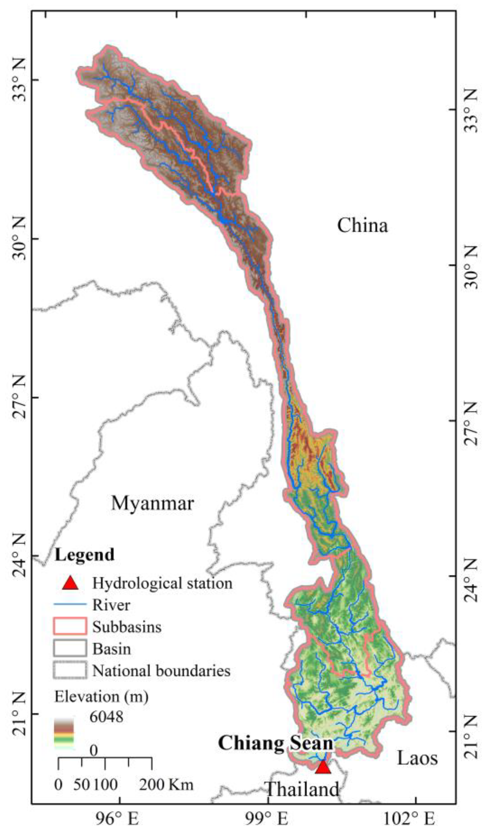
2.1. Study Area

The upper Lancang-Mekong River is one of the main rivers located in southwest China and is the most typical north–south river in the world (Figure 1), with a length of approximately 2129 km and a drainage area of 1.87 × 105 km². The LMRB spans the tropical, subtropical, and temperate climate zones and possesses unique hydrological characteristics, owing to its great regional variety. Due to the monsoon, the upper LMRB is dry and cold in winter and hot and humid in summer, and the annual precipitation in the region is distributed unevenly. The precipitation in the wet season in the LMRB accounts for the majority of the annual precipitation, and the seasonal changes are significant. Therefore, floods and droughts are the major natural disasters in the upper LMRB. According to statistical data acquired from the Yunnan Water Resources Department (http://wcb.yn.gov.cn/html/shuiziyuangongbao/, accessed on 30 December 2022), the average recurrence of floods in the upper LMRB is 9 years for major floods and 3 years for minor ones, and most floods occur between June and August. The average flooding frequency in this region is 3–5 years. These natural disasters have caused huge losses to agriculture in the downstream areas of the Mekong River, which include several developing countries. All these countries are highly dependent on agriculture, fishing, and hydropower; therefore, the forecasting, governance, and management of floods and droughts in these areas are extremely important.

2.2. Data

The NCEP CFSR represents a new generation of re-analysis product, which provided the best estimates of the land surface state from 1979 to 2014 and was developed from the global high-resolution atmosphere–ocean–land surface–sea ice coupling system and data assimilation system [35]. Notably, the CFSR datasets have a high resolution globally (T382L64). The CFSR datasets provide six meteorological variables for hydrological models, including precipitation, maximum/minimum temperatures, relative humidity, wind speed, and solar radiation. We downloaded daily meteorological variables in the SWAT file format from the SWAT data website (https://swat.tamu.edu/data/cfsr, accessed on 16 December 2021). In order to perform grid-to-grid comparison between CFSR and CMADS meteorological re-analyses, the coordinates of CFSR were interpolated into those of CMADS by the bilinear interpolation method. Although the resolution difference between CMADS and CFSR is small, their data coordinates deviated slightly, and there was a certain level of spatial error in the interpolated CFSR data.

In contrast to the global CFSR datasets, CMADS is a regional re-analysis dataset developed by Dr. Meng Xianyong, mainly covering East Asia (0°–65° N, 60°–160° E). The CMADS product was constructed through the assimilation and correction of meteorological observations (automatic stations, satellites, and radars) and the European Centre for Medium-Range Weather Forecasts background field using multiple technologies and scientific methods, including resampling, bilinear interpolation, and the loop nesting of data [36]. The assimilation process of CMADS was mainly achieved through LAPS and STMAS. CMADS is available to the public, which is beneficial for the areas of East Asia, especially the regions with relatively scarce meteorological data. CMADS includes multiple versions of the datasets with different resolutions (1/3°, 1/4°, and 1/8°) to meet different user needs. We used CMADS version 1.0 (1/3°) in this study, which is freely available (http://www.cmads.org/, accessed on 5 March 2022). We chose the common 6-year period (i.e., 2008–2013) to evaluate the CFSR meteorological datasets for the upper LMRB.

In addition to meteorological forcings, other land surface data were needed for delineating the watershed, including DEMs, land use, and soil type. The 90 m DEMs were acquired from the National Aeronautics and Space Administration and the Department of Defense’s National Imagery and Mapping Agency. The land use data were obtained from the Earth Resources Observation and Science Center, which adopts the USGS LULC 24 classification standard. The soil type data were required from the Food and Agriculture Organization of the United Nations [37] and were published in 2003 (https://www.fao.org, accessed on 20 December 2021). The gauged streamflow at the Chiang Sean hydrological station was obtained from the Mekong River commission.

There are eight main LULC types in the upper LMRB (Table S1): grassland, mixed forest, evergreen broad-leaved forest, tundra, savanna, deciduous broad-leaved forest, shrub land, and irrigated farmland and pasture. The coverage areas of grasslands and mixed forests exceed half of the total watershed area and are mainly distributed in the upstream and downstream regions, respectively. Eleven soil types and two dominant soil textures (loam and sandy clay loam) have been identified in the upper LMRB (Table S2). More information on the soil types is provided in Table S2 of the Supplementary Materials. Based on these geographical data, the upper LMRB was delineated to achieve a stream network based on the QGIS interface for SWAT+ 2.0. We created four subbasins from the DEM by specifying area thresholds and the outlet. To ensure accurate HRU landscape units to separate floodplain and upslope areas, we created 110 landscape units by demarcating the floodplain simply as a buffer drawn around the stream reaches. For each landscape unit, the largest potential HRU was chosen to be the dominant HRU, sharing the same land use, soil, and slope range [38]. The streamflow was generated from each HRU separately, and then the route to obtain the total streamflow for the watershed was determined, which provided a much better physical description of the water balance [39,40].

2.3. Evaluation Index

The performance of the CFSR meteorological datasets was evaluated for the common 6-year period (2008–2013) using R, PBIAS, and RMSE. R was used to measure the correlation between the variables of CFSR and CMADS; if the R value was close to 1, the two variables were considered to be linearly related. Furthermore, PBIAS was employed in this study as a measure of the average trend of CFSR greater or less than CMADS [41,42]. The optimal PBIAS value was considered as 0 (%). Low absolute values indicated an accurate model simulation; for example, ±25% represented good performance. A positive PBIAS value indicated an overestimation (by the model), whereas a negative value indicated an underestimation. Finally, the RMSE was used for measuring the differences between the values predicted by the model and the observed values, with a smaller value indicating better model performance.

$$\mathrm{R}=\frac{\sum \left({\mathrm{X}}_{\mathrm{t}}-\overline{\mathrm{X}}\right)\left({\mathrm{Y}}_{\mathrm{t}}-\overline{\mathrm{Y}}\right)}{\sqrt{\sum {\left({\mathrm{X}}_{\mathrm{t}}-\overline{\mathrm{X}}\right)}^2}\sqrt{\sum {\left({\mathrm{Y}}_{\mathrm{t}}-\overline{\mathrm{Y}}\right)}^2}},$$

(1)

$$\mathrm{PBIAS}=\frac{{\displaystyle \sum }\left({\mathrm{X}}_{\mathrm{t}}-{\mathrm{Y}}_{\mathrm{t}}\right)\times 100}{{\displaystyle \sum }{\mathrm{Y}}_{\mathrm{t}}},$$

(2)

$$\mathrm{RMSE}=\sqrt{\frac{1}{\mathrm{N}}{\displaystyle \sum }{{(\mathrm{X}}_{\mathrm{t}}-{\mathrm{Y}}_{\mathrm{t}})}^2},$$

(3)

where X_t indicates the meteorological variables of the CFSR datasets; Y_t indicates the meteorological variables of the CMADS datasets, including six mereological elements; and $\overline{\mathrm{X}}$ and $\overline{\mathrm{Y}}$ indicate the average values of the CFSR and CMADS meteorological variables, respectively.

The Nash–Sutcliffe efficiency coefficient (NSE), the coefficient of determination (R²), and PBIAS were used to evaluate the hydrological model simulations based on the CFSR and CMADS meteorological datasets for the common 6-year period (2008–2013). The NSE reflected the degree of fit between the monthly simulated and observed streamflow at the Chiang Sean hydrological station [43]. If the NSE approached 1, it indicated the most accurate hydrological simulation. Moriasi et al. [44] recommended the use of performance ratings to measure SWAT performance. For the monthly time step, 0.75 < NSE < 1 and PBIAS < ±10% indicated that the hydrological simulations were very good. Values of 0.65 < NSE < 0.75 and ±10% ≤ PBIAS ≤ ±15% indicated that the hydrological simulations were good; 0.50 < NSE < 0.65 and ±15% ≤ PBIAS ≤ ±25% indicated that the hydrological simulations were satisfactory; and NSE ≤ 0.5 and PBIAS ≥ ±25% indicated that the hydrological simulations were unsatisfactory. Note that R² was used to measure the accuracy of the simulated streamflow. The equations used to calculate the statistical indexes are shown below:

$$\mathrm{NSE}=1-\frac{{\displaystyle \sum }{{(\mathrm{Q}}_{\mathrm{o}}^{\mathrm{t}}-{\mathrm{Q}}_{\mathrm{m}}^{\mathrm{t}})}^2}{{\displaystyle \sum }{{(\mathrm{Q}}_{\mathrm{o}}^{\mathrm{t}}-\overline{{\mathrm{Q}}_{\mathrm{o}}^{\mathrm{t}}})}^2},$$

(4)

$${\mathrm{R}}^2=\frac{{({\displaystyle \sum }{(\mathrm{Q}}_{\mathrm{o}}^{\mathrm{t}}-\overline{{\mathrm{Q}}_{\mathrm{o}}^{\mathrm{t}}}){\displaystyle \sum }{(\mathrm{Q}}_{\mathrm{m}}^{\mathrm{t}}-\overline{{\mathrm{Q}}_{\mathrm{m}}^{\mathrm{t}}}\left)\right)}^2}{{\displaystyle \sum }{{(\mathrm{Q}}_{\mathrm{o}}^{\mathrm{t}}-\overline{{\mathrm{Q}}_{\mathrm{o}}^{\mathrm{t}}})}^2{\displaystyle \sum }{{(\mathrm{Q}}_{\mathrm{m}}^{\mathrm{t}}-\overline{{\mathrm{Q}}_{\mathrm{m}}^{\mathrm{t}}})}^2},$$

(5)

$$\mathrm{PBIAS}=\frac{{\displaystyle \sum }\left({\mathrm{Q}}_{\mathrm{m}}^{\mathrm{t}}-{\mathrm{Q}}_{\mathrm{o}}^{\mathrm{t}}\right)\times 100}{{\displaystyle \sum }{\mathrm{Q}}_{\mathrm{o}}^{\mathrm{t}}},$$

(6)

where ${\mathrm{Q}}_{\mathrm{o}}^{\mathrm{t}}$, ${\mathrm{Q}}_{\mathrm{m}}^{\mathrm{t}}$, $\overline{{\mathrm{Q}}_{\mathrm{o}}^{\mathrm{t}}}$, and $\overline{{\mathrm{Q}}_{\mathrm{m}}^{\mathrm{t}}}$ denote the monthly observed, simulated, observed average, and simulated average streamflows at time t, respectively.

2.4. Hydrological Models

The SWAT model aims to predict the long-term effects of land management practices on the production of water, sediment, and agricultural chemicals in large complex watersheds with different soil, land use, and management conditions [40]. Note that SWAT+ is a completely restructured version of SWAT. As a semi-distributed hydrological model, SWAT+ can effectively simulate the flow and pollutant transport of rivers under different conditions and scenarios across a wide range of spatiotemporal scales. Bieger et al. [39] concluded that the SWAT+ model is more flexible in terms of the delineation and interaction of the spatial objects in a watershed, offering users the opportunity to achieve a more realistic spatial representation of their target watershed areas.

In this study, we used a new and free SWAT+ version 2.0.6 model to perform hydrological modeling in the upper LMRB based on the QSWAT+ platform, which was the Quantum GIS 3.16 Interface for SWAT+. The SWAT+ model provided diverse options for physical processes at the watershed level. To drive the SWAT+ model, we used the Penman/Monteith method, the Soil Conservation Service’s curve number method, and the variable storage routing method to calculate the PET, estimate surface runoff, and determine the route of streamflow in the channel, respectively.

2.5. SWAT+ Parameter Sensitivity Analysis and Calibration Tool

In our study, we used the new and free SWAT+ toolbox v1.0 to carry out the parameter sensitivity analysis (SA), as well as calibration and validation, for the upper LMRB. The Sobol method, a quantitative SA method available in the SWAT+ toolbox, was used in this study for the upper LMRB and could indicate the degree of sensitivity of the parameters according to the contributions of each parameter to the final output results [45,46]. SA is the identification of parameters that are sensitive to the hydrological processes in different study areas [47,48]. Based on several studies [45,49,50], we considered 24 commonly used parameters, along with their previously established reference ranges, for the parameter sensitivity analysis. For Sobol’s quantitative SA, we specified 100 random sample points for 24 tunable parameter ranges, resulting in 5000 parameter samples [51,52]. We obtained the first-order sensitivity results of each parameter after 5000 SWAT+ model simulation runs. The sensitivities of the parameters were ranked by the absolute value of the first-order sensitivity. After determining the model-sensitive parameters, we calibrated them using the observed streamflow obtained from Chiang Sean station as a reference. In order to represent the realistic physical process in the SWAT+ model, we used the calibration procedure to improve the fitting degree between simulated and observed streamflow [53]. The SWAT+ toolbox provided a dynamically dimensioned search (DDS) automatic calibration algorithm [54], which could automatically expand the search to find a good solution without tuning the algorithm parameters. The DDS automatic calibration algorithm has outstanding performance in terms of both convergence speed and parameter set searching ability [55,56]. Finally, we validated the optimal parameter values of the SWAT+ model for the streamflow simulation. According to the time length of the meteorological datasets and the observed streamflow from the Chiang Saen station, we chose 2008 as the warm-up period, 2009–2010 as the calibration period, and 2011–2013 as the validation period.

3. Results

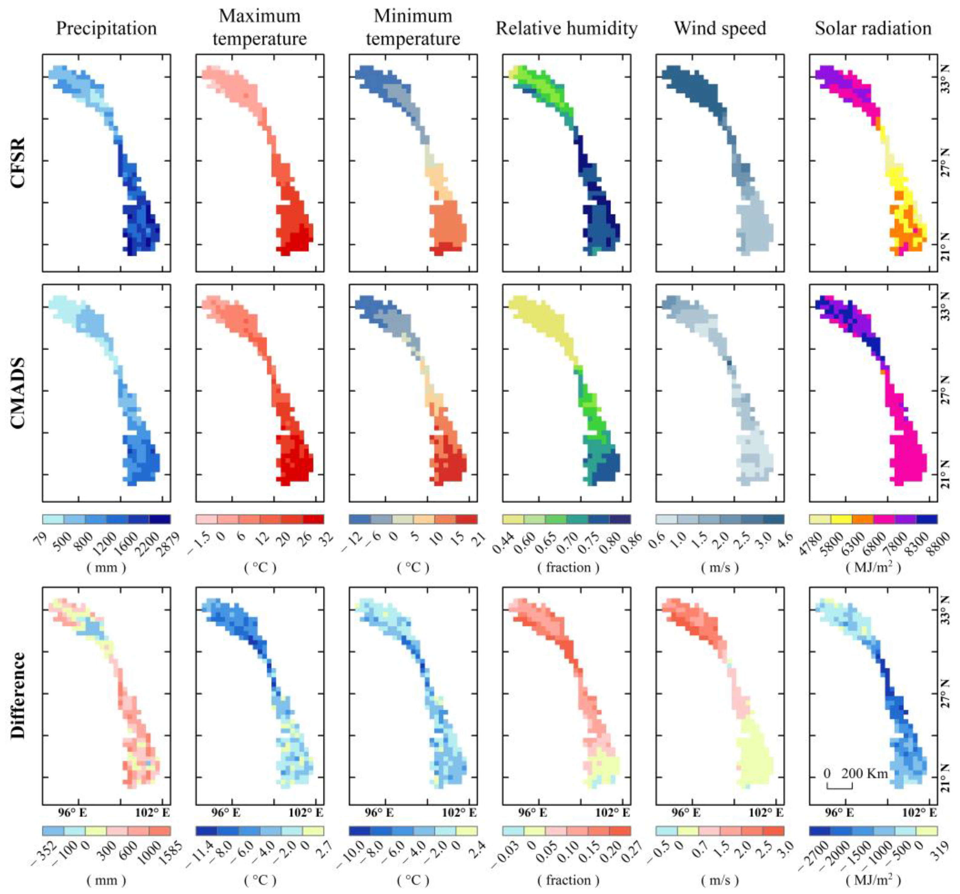
3.1. Spatial Annual Average Distribution of CFSR Dataset and the Difference for LMRB

We evaluated six meteorological variables of the CFSR dataset using a multi-source meteorological dataset (CMADS). For grid-to-grid comparisons, we consistently interpolated the spatial resolution of the two datasets to 0.3°, about 33.3 km. The difference maps were computed by subtracting the average annual meteorological variables of the CMADS dataset from the average annual values of the CFSR dataset. Figure 2 portrays the annual average of the six meteorological variables from 2008 to 2013 and the differences between the average annual values of the CFSR and CMADS datasets. The spatial distributions of the annual mean precipitation values of these two datasets were highly similar, indicating less precipitation in the northwest region and more precipitation in the southeast region. However, the average annual precipitation of the CFSR dataset was generally 300–600 mm higher than that of the CMADS dataset across the whole basin, with the range being 252–1488 mm in the CMADS dataset and 429–2495 mm in the CFSR dataset. Some studies have found that the precipitation is often overestimated by CFSR datasets [3,30,57]. These studies indicated that the degree of overestimation of the CFSR data for 2008–2013 was more noticeable than that of other precipitation products; the increase in the precipitation was significant circa 2006. These phenomena may be attributed to single-point observation errors [30,57]. However, there was an exception in that the CFSR dataset contained an area of less than 300 mm annual precipitation in the upper part of the basin. Lauri et al. [11] also presented data showing a lower average annual precipitation in the upper LMRB over the 1999–2005 period. Lorenz and Kunstmann [24] also concluded that there seemed to be a significant bias in the estimation of precipitation at mid to high latitudes by CFSR, which could be explained by the excessive activity in the daily cycle of atmospheric composition over North America [58]. Additionally, some studies found that CMADS often underestimates precipitation, because the daily precipitation recorded by CMORPH satellites always underestimates light rainfall events (due to the interference of surface reflectivity) [3,26,59]. Furthermore, complex orographic features, as well as the effects of the Pacific and Indian Ocean monsoons, may influence the high spatial heterogeneity of precipitation, thus reducing the accuracy of the precipitation predictions by both CMADS and CFSR [3].

The spatial distributions of the annual mean max/min temperatures in the CFSR and CMADS datasets were highly similar; the temperature increased gradually from the upper to lower reaches of the basin. However, both the average annual max and min temperatures of the CFSR dataset were generally lower than those of the CMADS dataset; notably, the maximum temperature of the CFSR dataset was lower in the upper part of the basin, with a negative 6 ℃ bias. The minimum temperature of the CFSR dataset was generally lower across the whole basin, and there were no significant regional differences. Lauri et al. [11] also found that the average annual temperature was lower in the upper LMRB over the 1999–2005 period. Liu et al. [3] found that the maximum and minimum temperatures of CMADS and CFSR were both underestimated in the Qinghai-Tibet Plateau. Wang et al. [57] found that the CFSR temperature anomaly in tropical regions was greater than that at mid to high latitudes.

Notably, the spatial distribution of the annual relative humidity was consistent with that of the annual precipitation, with lower relative humidity in the northwest and higher relative humidity in the southeast. The relative humidity of the CFSR dataset was generally higher than that of the CMADS dataset across the whole basin. Precipitation and temperature are the key factors that affect relative humidity, which may be the main reason why the CFSR dataset had a higher relative humidity than the CMADS dataset. Some studies found that the relative humidity values in the CFSR dataset were inaccurate [3,60], as they were higher than the observed values [60]. The spatial distributions of the annual wind speed in the CFSR and CMADS datasets were similar, but the wind speed in the CFSR dataset was significantly higher than that in the CMADS dataset in the upper part of the basin, by approximately 2 m/s. We noted that the wind speed was high in the plateau area and decreased gradually with decreasing elevation. It has been demonstrated that wind speed is overestimated by CFSR and CMADS compared with observed wind speeds in high-altitude regions [3,61]. Another significant difference between the CFSR and CMADS datasets was solar radiation. The annual solar radiation of the CFSR dataset was significantly lower than that of the CMADS dataset; in particular, the solar radiation was 1500 MJ/m² lower in the downstream region.

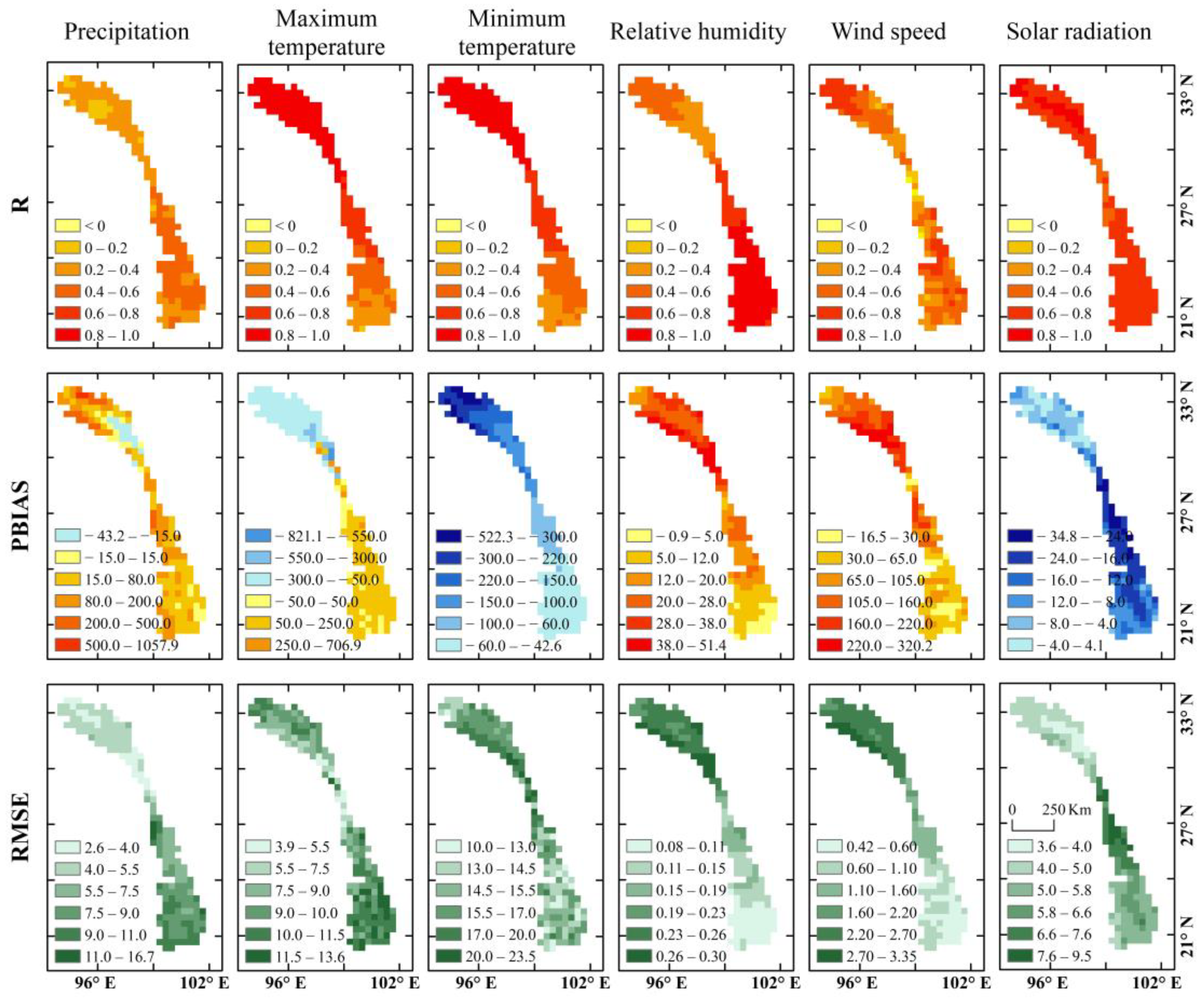
3.2. Evaluating the Meteorological Variables of CFSR in the Upper LMRB

After comparing the annual average spatial distribution of the CFSR dataset in the upper LMRB, we evaluated the applicability of the meteorological variables of the CFSR when CMADS was considered as the observational reference. The evaluation indices included R, PBIAS, and RMSE, and the calculation was based on the daily meteorological variables for 1 January 2008 to 31 December 2013. The spatial distributions of the R, PBIAS, and RMSE values of the six meteorological variables in CFSR and CMADS are shown in Figure 3. In terms of precipitation, the R values increased from the upstream region to the downstream region from 0.14 to 0.56, indicating that the precipitation values in the CFSR dataset were more accurately modeled in the downstream region. The values of PBIAS were positive across almost the whole basin, which implied that the amount of precipitation in the CFSR dataset was higher than that in the CMADS dataset. The highest positive PBIAS values (above 500) were in the upper part of the basin. However, negative PBIAS values were also identified in the upper part of the basin, implying that the amount of precipitation in the CFSR dataset was lower than that in the CMADS dataset. Future research is needed to explain this contradiction. The RMSE values increased from the upstream region (2.6) to the downstream region (16.7), indicating that there was a larger deviation in precipitation in the downstream region and a smaller deviation in the upstream region.

In terms of the max/min temperatures, the R values were positive and high over the entire LMRB, reaching a maximum of 0.95. This indicated that the maximum and minimum temperatures of the CFSR dataset were accurate for most areas. However, there were deviations in the PBIAS and RMSE values. The PBIAS values for the maximum temperature were negative in the upstream region but positive in the downstream region, indicating that the maximum temperatures of the CFSR dataset were lower than those of the CMADS dataset in the upstream region but higher than those of the CMADS dataset in the downstream region. Notably, the greatest positive (706.9%) and negative (–821.1%) PBIAS values for maximum temperature were observed in the middle and upper reaches of the upper LMRB, implying a great deviation in the maximum temperature values between CFSR and CMADS. The PBIAS values for the minimum temperature were negative across the whole basin, indicating that the minimum temperatures of the CFSR dataset were lower than those of the CMADS dataset. The most negative PBIAS values were observed in the upstream region and decreased gradually from the upstream to the downstream regions. The RMSE values for the maximum and minimum temperatures were similar to the PBIAS results, but the RMSE of the maximum temperature was generally smaller than that of the minimum temperature (10.0 compared to 23.5).

The R values of the relative humidity in the two datasets portrayed a stronger positive correlation in the downstream regions, and the PBIAS and RMSE values of the relative humidity were small in the downstream regions, indicating that the two datasets were highly similar in the downstream regions. However, the deviations in the relative humidity were rather large in the upstream regions, with the CFSR values being higher than the CMADS values. The R values of the wind speed were moderate, while the PBIAS and RMSE values were small in the upstream regions, indicating that the wind speed of the CFSR dataset was closer to that of the CMADS dataset in the downstream regions. However, the deviations in wind speed were positive and large in the upstream regions, where the wind speed of the CFSR dataset was higher than that of the CMADS dataset. The R value of the solar radiation between the CFSR and CMADS datasets was high over the entire basin, and the PBIAS and RMSE values were small in the upstream regions, indicating that the solar radiation of the CFSR dataset was closer to that of the CMADS dataset in the upstream regions. However, the deviations in solar radiation were negative and large in the downstream regions, where the solar radiation of the CFSR dataset was lower than that of the CMADS dataset.

The area average values of the statistical indicators for the six CFSR meteorological variables are shown in

Table 2. Area average values of the statistical indicators for the six meteorological variables between CFSR and CMADS.

Meteorological Variables	R	PBIAS	RMSE
Precipitation	0.35	85.47	6.68
Maximum temperature	0.68	−18.45	9.39
Minimum temperature	0.65	−127.71	15.71
Relative humidity	0.65	20.01	0.18
Wind speed	0.47	103.36	1.52
Solar radiation	0.72	−12.11	5.45

. Note that the indicators for maximum temperature, relative humidity, and solar radiation of the CFSR dataset were close to those of the CMADS dataset, with strong correlations (R ≥ 0.65) and small negative deviations (PBIAS ≤ 25%), but the precipitation and wind speed of the CFSR dataset presented low correlations (R ≤ 0.50) and large positive deviations (PBIAS ≥ 25%) compared to those of the CMADS dataset. The minimum temperatures of the CFSR dataset had a high correlation (R is 0.65) and large negative deviations (PBIAS = –127.71%) compared to those of the CMADS dataset. The temperature data portrayed the highest RMSE values, in the range of 9–16. The precipitation and solar radiation portrayed moderate values, and the relative humidity and wind speed parameters exhibited the smallest errors.

3.3. Comparison of the Hydrological Features between CFSR-Based SWAT+ and CMADS-Based SWAT+

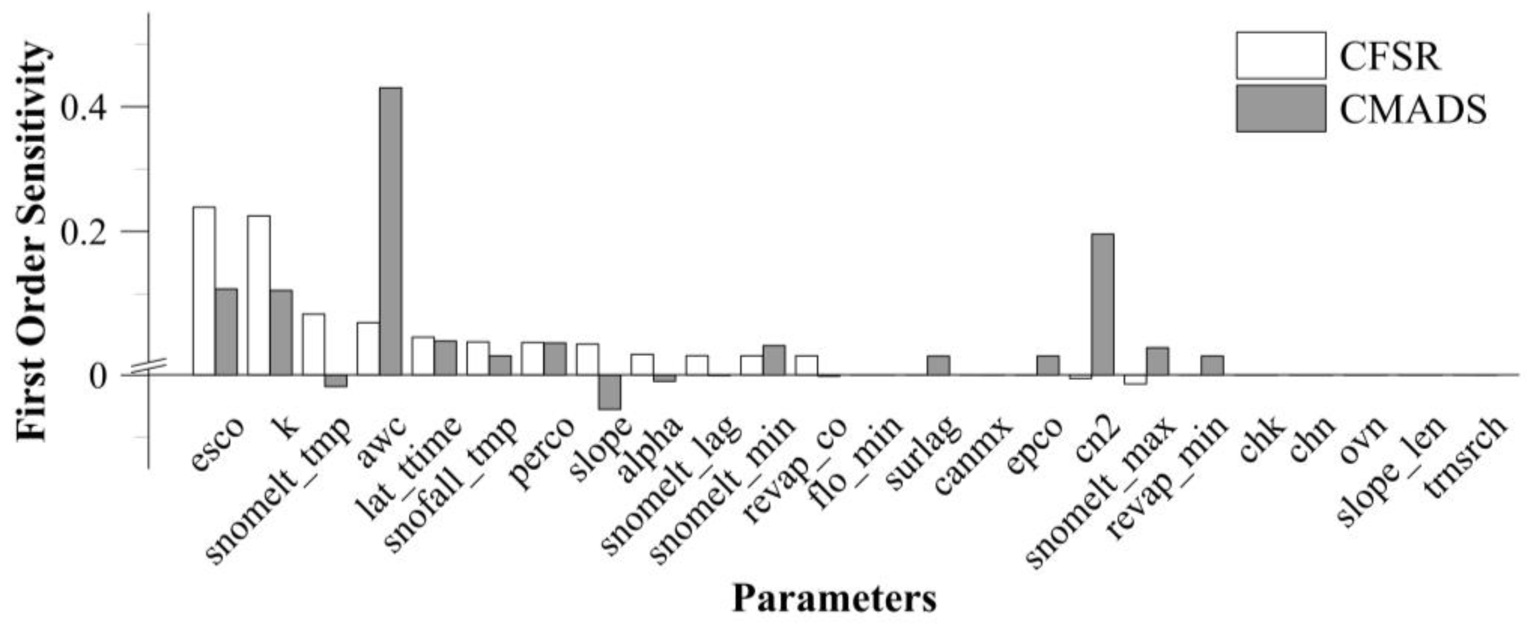
3.3.1. Model Parameter Sensitivity Based on CFSR and CMADS

In order to compare the hydrological features based on the two different meteorological re-analyses in the upper LMRB, we first needed to compare the model parameter sensitivity. We used Sobol’s method to screen the sensitive parameters. Figure 4 portrays the first-order sensitivities of a total of 24 commonly used parameters based on the two different meteorological re-analyses, CFSR and CMADS. We noted that the sensitive parameters based on CFSR for which the first-order sensitivity was greater than 0 were highly consistent with those based on CMADS. However, the sensitivities of these parameters (in terms of both datasets) were different. Overall, we determined 17 consistent sensitive parameters: esco, k, snomelt_tmp, awc, lat_ttime, snofall_tmp, perco, slope, alpha, snomelt_lag, snomelt_min, revap_co, surlag, canmx, epco, cn2, and snomelt_max. Two sensitive parameters were inconsistent: flo_min, which was sensitive based on CFSR only, and revap_min, which was sensitive based on CMADS only. Finally, we chose all 19 sensitive parameters, both consistent and inconsistent, for which the first-order sensitivity was greater than 0 for both CFSR and CMADS to carry out parameter calibration and validation.

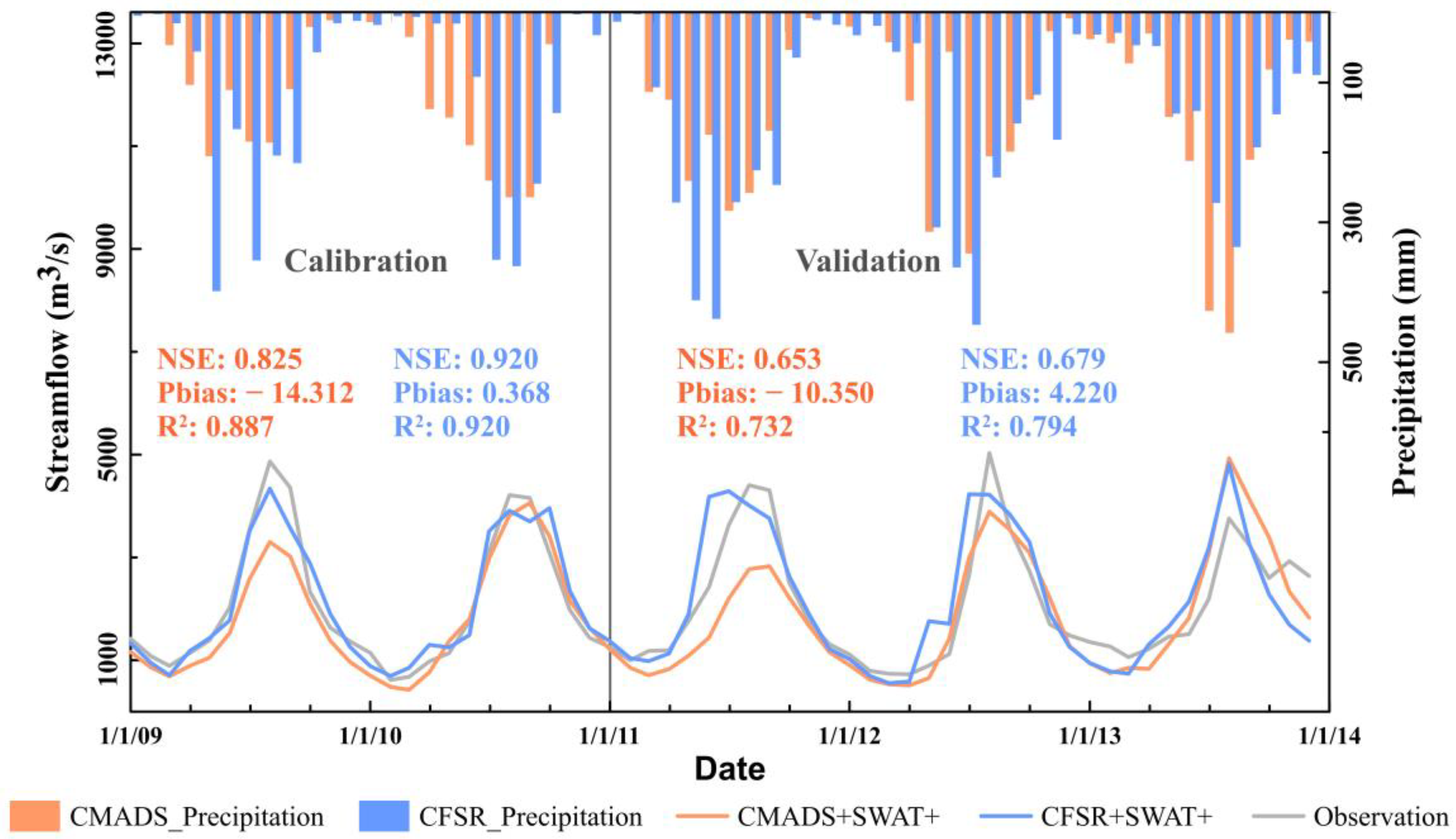
3.3.2. Model Calibration and Validation Based on CFSR and CMADS

To further assess the capability of the SWAT+ hydrological model for streamflow simulations based on the two different meteorological re-analyses in the upper LMRB, we employed DDS for model parameter calibration and streamflow simulation for validation using the monthly streamflow observed at Chiang Sean hydrological station. The hydrological simulation period was from January 2008 to December 2013. We chose the year 2008 as the warm-up period; the two years from 2009 to 2010 as the calibration period; and the three years from 2011 to 2013 as the validation period.

Table 3. The calibrated optimal values of the 19 sensitive parameters for SWAT+ based on the two meteorological re-analyses, namely, CFSR and CMADS.

Parameter	Description	Min	Max	Change Type *	Parameter Group	Optimal Value
						CFSR	CMADS
esco	Soil evaporation compensation factor (-)	0	1	replace	HRU	0.274	0.072
slope	Average slope steepness in HRU (m/m)	−50	50	relative	HRU	2.377	47.689
revap_co	Fraction of pet to calculate revap (-)	0.02	0.2	replace	Aquifer	0.184	0.198
epco	Plant water uptake compensation (-)	0	1	replace	HRU	0.046	0.717
canmx	Maximum canopy storage (mm_H2O)	0	100	replace	HRU	46.584	30.641
surlag	Surface runoff lag time (days)	0.05	24	replace	Basin	2.738	13.966
alpha	Alpha factor for gw recession curve (1/days)	0	1	replace	Aquifer	0.075	0.264
awc	Available water capacity of soil layer (mm_H2O/mm_soil)	−25	25	relative	Soil	15.516	−15.443
cn2	SCS runoff curve number adjustment factor SCS (%)	−20	20	relative	HRU	−19.682	−18.928
flo_min	Minimum aquifer storage to allow return flow (mm)	0	5000	replace	Aquifer	1704.311	3329.009
k	Saturated hydraulic conductivity of soil layer (mm/hr)	−80	80	relative	Soil	78.688	42.922
lat_ttime	Lateral flow travel time (days)	0.5	180	replace	HRU	118.878	126.252
revap_min	Threshold depth of water in shallow aquifer required to allow revap to occur (mm)	0	500	replace	Aquifer	451.913	231.766
snofall_tmp	Snow fall temperature (℃)	−5	5	replace	HRU	3.482	4.602
snomelt_lag	Snowmelt lag factor (-)	0	1	replace	HRU	0.591	0.976
snomelt_max	Maximum snow melt factor (mm/(d·℃)	0	10	replace	HRU	3.314	0.235
snomelt_min	Minimum snow melt factor (mm/(d·℃)	0	10	replace	HRU	8.177	4.773
snomelt_tmp	Snow melt temperature (℃)	−5	5	replace	HRU	−2.919	−3.637
perco	Percolation coefficient	0	1	replace	HRU	0.901	0.773

Note: * Relative change—increases/decreases the current value by a specified value; replace—the specified value takes the place of the old parameter value.

portrays the calibrated optimal values and the value range and change types of the 19 sensitive parameters for each meteorological re-analysis. The calibrated optimal values of the 19 sensitive parameters were very different for the two meteorological re-analyses, with these differences reflected mainly in the most sensitive parameters, including esco, slope, epco, and surlag. Notably, the optimal values of the parameters were positive for CFSR but negative for CMADS. This was seen, for example, in awc. Note that esco, revap_min, and awc all affected the process of evaporation. To adjust for the higher precipitation in CFSR, the evaporation based on CFSR may have required a greater value. However, the calibrated optimal values of some parameters were consistent, including revap_co, cn2, lat_time, and perco. Based on the results comparison of the re-analyses, as explained in Section 4.1 and Section 4.2, the differences in the meteorological re-analyses may have been the reason for the different calibrated optimal values.

Two simulated monthly streamflows, based on the corresponding calibrated SWAT+ model parameters forced by the two different meteorological re-analyses, with the monthly streamflow observed at the Chiang Sean hydrological station during the calibration period (2009–2010) and validation period (2011–2013), are shown in Figure 5. The statistical measures used to evaluate the simulated streamflow included the NSE coefficient, PBIAS, and R². The higher the values of the NSE and R², the smaller the PBIAS value and the more accurate the simulated streamflow. Both monthly streamflow simulations performed well during the calibration period, with NSE values greater than 0.8, R² values greater than 0.88, and PBIAS values lower than 15%. The performances were still good during the validation period, with NSE values greater than 0.65, R² values greater than 0.70, and PBIAS values lower than 11%. Overall, the model performance driven by the CFSR dataset was better than that driven by the CMADS dataset, with higher NSE and R² values and smaller PBIAS values. According to the hydrograph in Figure 5, the CFSR-based and CMADS-based SWAT+ streamflow simulations could essentially predict the observed peak and low streamflow, but the CMADS-based SWAT+ streamflow simulation tended to underestimate the peak and low streamflow. Therefore, we noted that CFSR met the demands for simulating streamflow through the SWAT+ hydrological model in the upper LMRB.

To understand the mechanism behind the simulated monthly streamflow, we analyzed the simulated water balance based on the corresponding calibrated SWAT+ model parameters forced by the two different meteorological re-analyses, as shown in Figure 6, which were obtained from the model check component in the SWAT+ editor. Although the precipitation in the CFSR-based SWAT+ simulation was much higher than that in the CMADS-based SWAT+ simulation across the entire basin, only 49% of the CFSR precipitation was converted to streamflow, while 82% of the CMADS precipitation was converted. Furthermore, the evaporation and transpiration (ET) in the CFSR-based SWAT+ simulation were also higher than those in the CMADS-based SWAT+ simulation, which may have been another reason why the CFSR-based and CMADS-based SWAT+ streamflow simulations did not differ greatly. The higher percolation in the CMADS-based SWAT+ simulation may have led to the lower simulated peak and low streamflow. Several factors could have caused different responses between the meteorological estimates and hydrological outputs, including the sensitive parameters and their calibrated optimal values in the SWAT+ hydrological model. Gao et al. [25] concluded that the conversion of precipitation to runoff is a highly complex nonlinear process. Therefore, the discrepancies between the two meteorological forcings did not transfer linearly to runoff. This may have resulted in significant differences in the simulated streamflow forced by the two different meteorological re-analyses, CFSR and CMADS.

4. Discussion

The discussion will revolve around three topics. First, we discuss the similarities and differences in the two gridded meteorological forcings between our results and other results in Section 4.1. Then, we discussed the factors that may affect hydrological modeling and hydrological responses in Section 4.2, including the time span of meteorological forcings, the length of model calibration and validation periods, the parameter sensitivity values, and the criteria for parameter selection. Finally, we summarize the limitations of this study and the future research directions in Section 4.3.

4.1. Differences in Meteorological Forcings

Several previous studies have compared the meteorological elements of global or local re-analyses with gauge-observed data [11,24,25,26,30]. Such comparisons may introduce errors and uncertainties between the re-analyses and the gauged observations due to spatial scale differences. However, a comparison between re-analyses and grided observed data, such as CMADS data, can improve our understanding of how meteorological elements behave [62]. After comparing the precipitation and temperature values between global atmospheric re-analyses and observed data, Tian et al. [62] concluded that the precipitation values of CFSR were higher than the observed data and CMADS, while the maximum/minimum temperatures of CFSR were generally lower than the observed data and CMADS. These findings are also consistent with the results of another study on the Mekong River Basin [11].

The comprehensive meteorological CMADS datasets rendered the comparison of the other meteorological variables (wind speed, relative humidity, and solar radiation) for the CFSR in the upper LMRB possible. Our results showed that the precipitation, relative humidity, and wind speed of CFSR were higher than those of CMADS, while the max/min temperatures and solar radiation were lower than those of CMADS. There is a need to investigate the reason why the temperatures and solar radiation of the CFSR dataset were lower than those of the CMADS dataset and why CFSR exhibited higher wind speeds than the CMADS dataset. Meng et al. [36] concluded that temperature had a relatively greater RMSE in the southern and western parts of the Yunnan province, and a minority of stations in the region showed negative biases when compared to the observations from the national automatic stations. Relative humidity and wind speed showed a positive bias effect in the southern parts of the Yunnan province [36]. However, the factors influencing the accuracy of CMADS have not yet been systematically analyzed [36]. The main reason for the differences between the CMADS and CFSR datasets was the difference in the observation data sources and assimilation methods [35,36].

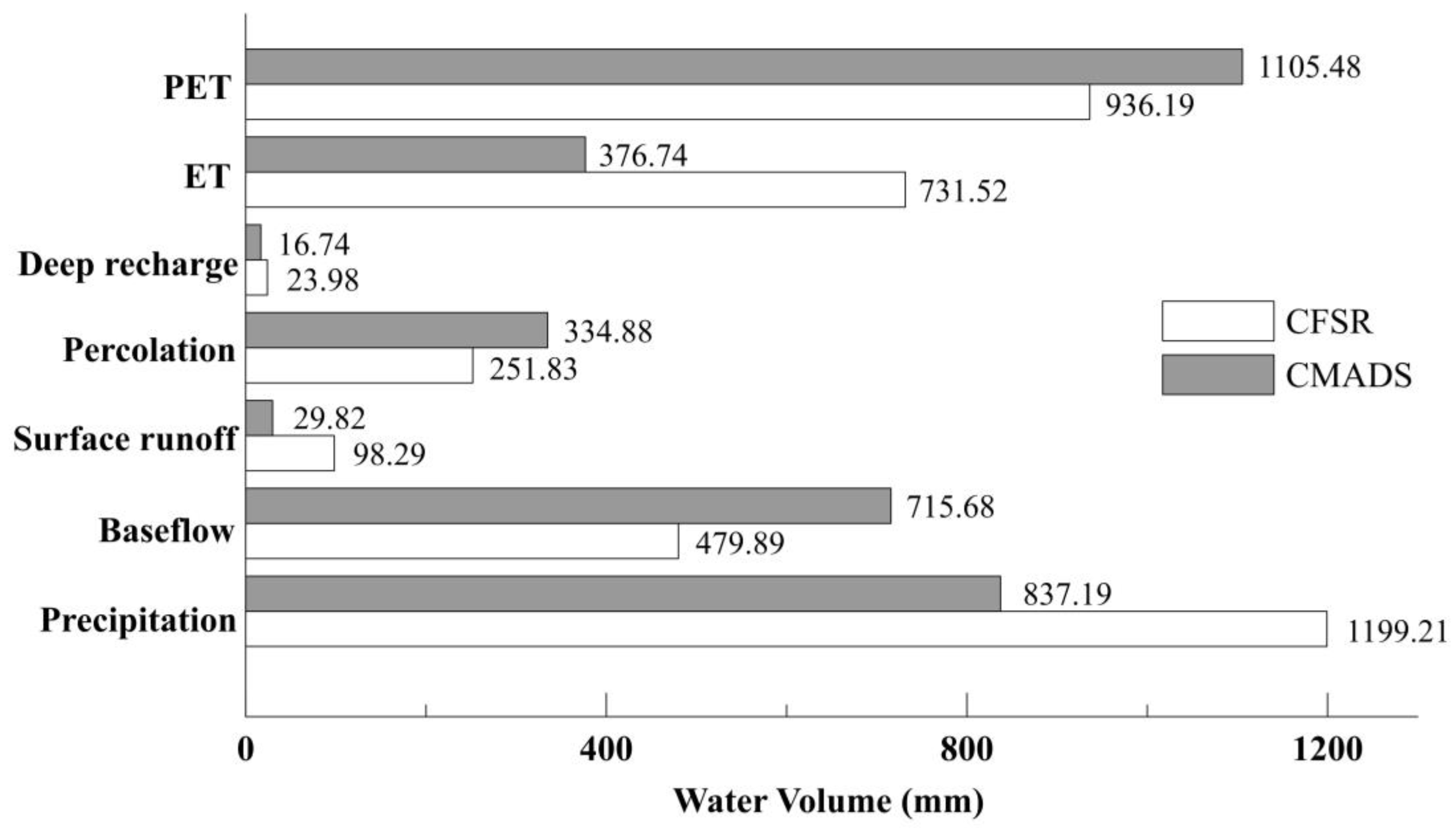
4.2. Differences in Hydrological Model Response

Various studies have reported that the performance of meteorological re-analyses in discharge modeling varies depending on the situation compared to rain gauge data [2,3,11,25,26,27,30]. However, their results indicate that CFSR could be a valuable option for hydrological simulation in areas with limited data. In this study, we compared the hydrological responses between the CFSR-based SWAT+ simulation and CMADS-based SWAT+ simulation under the same watershed delineation, hydrological model, parameter sensitivity analysis, and calibration method. However, the two different meteorological re-analyses led to different sensitivities and calibrated optimal values for the consistent parameters, which further led to different hydrological responses. Moreover, the simulations based on CFSR and CMADS yielded significant differences in the water balance components in the upper LMRB. For example, higher precipitation led to a lower conversion rate to streamflow and higher evaporation and transpiration according to the water balance. Therefore, a different watershed delineation, hydrological model, parameter sensitivity analysis, and calibration method would lead to different hydrological responses. In order to make the hydrological simulation more efficient in evaluating the performance of the meteorological re-analyses in discharge modeling, we created four subbasins and 110 HRUs from the DEM by specifying the default area thresholds for channels (1716 km²) and streams (17,160 km²). As the small area thresholds created more subbasins and HRUs, they required more computing time for the hydrological simulation, which may have affected the hydrological responses.

The common six-year time span of meteorological forcings in the hydrological modeling was short in this study. The global gridded meteorological re-analysis, CFSR, included a nearly 35-year period which met the long-term time-series requirements of hydrological modeling, but the regional gridded meteorological re-analysis, CMADS, only covered a 10 years period. However, regional gridded meteorological re-analyses generally assimilate more observations than global ones; resolve physical processes at a finer scale; and consequently account for terrain characteristics, topography, land use, and local weather characteristics [63]. In order to compare their performances in hydrological modeling and verify the performance of the global gridded meteorological re-analyses, we chose the common six-year period (i.e., 2008–2013). If the global gridded meteorological re-analysis-based hydrological modeling performed better than or comparably to the regional gridded meteorological re-analysis-based hydrological modeling, the global gridded meteorological re-analysis, here CFSR, would be chosen for the hydrological modeling research, because CFSR includes long-term time series and covers the global spatial scale.

The common six-year time span of the two meteorological forcings for hydrological modeling was from January 2008 to December 2013. No definite conclusions have been drawn as to the lengths of observed streamflow necessary for effective model calibration [64], but the record requires sufficiently diverse flow conditions. The lengths of time used in this study impacted the hydrological responses, because some extreme interannual variability was not included. We chose 2008, one year, as the warm-up period. According to the same physical criteria as the calibration and validation periods [53,65], such as the same type of climate and land use, the two years from 2009 to 2010 were used as the calibration period and three years from 2011 to 2013 as the validation period. The average values of the observed streamflow at Chiang Sean station in 2009–2010 and 2011–2013 were 2097.04 m³/s and 2069.69 m³/s, respectively, and the variances were 1,680,030.8 (m³/s)² and 1,347,166.8 (m³/s)², which met the same physical criteria as the calibration and validation periods. The same duration of model calibration and validation was set according to research on the Qinghai-Tibet Plateau [3]. Therefore, the hydrological modeling performances based on the two meteorological gridded re-analyses were to a certain extent credible.

In this study, we used a quantitative sensitivity analysis method, Sobol’s method, which could evaluate the impacts of each parameter (first-order effects) and its interactions (interaction effects) with other parameters on the model output [46,52]. Sobol’s method calculates the contribution of the variance due to the perturbation of each parameter relative to the total variance of the model output [51]. We obtained the first-order sensitivities of 24 common parameters after 5000 SWAT+ model simulation runs based on the SWAT+ toolbox v1.0. The sum of the first-order sensitivity values of the 24 common parameters was one or less than one, and the first-order sensitivity values were well differentiated based on Sobol’s method: some sensitivity values were higher (e.g., esco for CFSR was 0.24, and k for CFSR was 0.22), and some sensitivity values were lower (e.g., flo_min for CFSR was −0.0000013). However, the first-order sensitivity values were more uniform when using other quantitative sensitivity analysis methods, such as the McKay main effect analysis method [66]. Many studies [51,67] recommend that sensitive parameters should be chosen when the absolute value of the first-order sensitivity according to Sobol’s method is greater than 0. Another reason for the low sensitivity value may have been that the interaction between parameters was not considered in this study. Gan et al. [66] concluded that parameters with lower main effect values may have significant interaction effects with other parameters, which should also be treated as important parameters. Therefore, we chose all parameters with a first-order sensitivity value greater than 0 instead of filtering parameters by setting sensitivity thresholds to avoid missing important sensitive parameters.

The uncertainty of precipitation estimations and meteorological forcings is regarded as typical for input data [68], and Leta et al. [69] concluded that it is very important to take rainfall uncertainty into account when calibrating a hydrological model. It was difficult to perform bias correction on the precipitation data in this study because the weather gauge stations were scarce. We could have feasibly used the satellite-based observational precipitation datasets to correct the precipitation values. We also needed to correct the biases of the other meteorological forcings; however, fewer of these forcings were comprehensively observed, such as relative humidity and solar radiation. The uncorrected bias in the meteorological forcings in this study resulted in uncertainties in the hydrological model parameters.

4.3. Limitations

In addition to the input meteorological data and hydrological model parameters, other limitations, including anthropogenic activities and climate change, could have influenced the hydrological modeling in the upper LMRB. Firstly, we did not consider anthropogenic activities in the hydrological modeling, such as the dam construction along the upper LMRB. The observed streamflow was affected by dam construction [14,70,71], but the simulated streamflow did not reflect this factor. Secondly, climate change may influence hydrological modeling, but the research period of this study was too short to include the impact of climate change. Another limitation was the limited number of observed hydrological stations for hydrological modeling in the upper LMRB. The upper LMRB is huge, topographically and hydrologically diverse, and spans areas affected by different sources of highly variable monsoonal moisture. We used only one observed streamflow from Chiang Sean hydrological station for hydrological modeling. We could compare the performance of the hydrological responses based on the two gridded meteorological re-analyses in more detail by dividing the upper LMRB into several parts.

The increases or decreases in streamflow caused by anthropogenic activities and climate change pose some challenges to the supply and management of water resources in the upper LMRB. Medium- to long-term streamflow forecasting is a good way to meet these challenges. Currently, the main problem with medium- to long-term streamflow forecasting is the low prediction accuracy, which makes it difficult to effectively guide production practice. In the present study, we focused on the performance of hydrological modeling in the LMRB based on different re-analysis datasets and concluded that CFSR could drive the SWAT+ model to simulate the streamflow in the upper LMRB. The available and valuable hydrological modeling based on CFSR provided an experimental basis for us to conduct ensemble streamflow prediction for medium- to long-term hydrological predictability research. We will use climate forecast data as the input data for the SWAT+ model to conduct ensemble streamflow prediction and focus on an analysis of how climate forecasts contribute to the predictability of seasonal streamflow in the upper LMRB, which could provide a scientific basis for realizing medium- and long-term streamflow forecasting, promoting the efficient development and utilization of water resources in the basin, and formulating effective flood control and drought relief measures.

5. Conclusions

Our study aimed to assess differences in hydrological responses through hydrological modeling in the upper LMRB using two common open-gridded meteorological datasets, CFSR and CMADS. This study evaluated the suitability of six meteorological variables from the CFSR and CMADS datasets that are commonly used to force SWAT+ models, along with analyzing the differences in the hydrological modeling. We arrived at the following conclusions:

All the meteorological variables of the CFSR and CMADS datasets exhibited similar spatial average annual distributions; however, the precipitation, relative humidity, and wind speed values in the CFSR dataset were greater than those in the CMADS dataset. Further, the temperatures and solar radiation were lower in the CFSR dataset. The spatial distributions of the statistical indicators in the CFSR and CMADS datasets, namely, the R, PBIAS, and RMSE values, were different. The temperatures and solar radiation values in the CFSR and CMADS datasets exhibited strong correlations across the entire basin, while precipitation and relative humidity portrayed strong correlations in the downstream regions. Additionally, wind speed exhibited an irregular spatial distribution of correlation over the entire river basin. The PBIAS results indicated that precipitation, relative humidity, and wind speed portrayed positive deviations across the entire basin. Minimum temperature and solar radiation portrayed negative deviations across the entire basin. Notably, the maximum temperature yielded a positive deviation in the downstream and a negative deviation in the upstream regions. These conclusions were further confirmed by the result of the RMSE and the area average values of the statistical indicators.

For a comparison of the hydrological features of the CFSR- and CMADS-based SWAT+ models, we compared the sensitive parameters and simulated the monthly streamflow. Different meteorological datasets resulted in significant differences in hydrological responses, which were reflected by the different sensitive parameters and their optimal values. Nineteen sensitive parameters (from a total of twenty-four parameters) for the CFSR and CMADS models were mostly the same, with only two being inconsistent, namely, flo_min and revap_min. However, the sensitivities of these parameters were different. The calibrated optimal values of the 19 sensitive parameters were very different for the two meteorological re-analyses, reflected mainly in the most sensitive parameters, including esco, slope, epco, and surlag. These different calibrated optimal values of the sensitive parameters lead to different simulated water balance components between the CFSR- and CMADS-based SWAT+ models. The monthly streamflow simulated using the CFSR-based SWAT+ model was superior to that simulated using the CMADS-based SWAT+ model from 2008–2013, with higher NSE and lower PBIAS values. These results indicated that CFSR could better drive the SWAT+ model to simulate the streamflow in the upper LMRB. This study advanced our understanding of the strengths and weaknesses of different meteorological forcings and their performance and helped to determine the hydrological models applicable for the upper LMRB.

References

1. Singh, V.P. Hydrologic Modeling: Progress and Future Directions. Geosci. Lett. 2018, 5, 15. [Google Scholar] [CrossRef]
2. Fuka, D.R.; Walter, M.T.; MacAlister, C.; Degaetano, A.T.; Steenhuis, T.S.; Easton, Z.M. Using the Climate Forecast System Reanalysis as Weather Input Data for Watershed Models. Hydrol. Process. 2014, 28, 5613–5623. [Google Scholar] [CrossRef]
3. Liu, J.; Shanguan, D.; Liu, S.; Ding, Y. Evaluation and Hydrological Simulation of CMADS and CFSR Reanalysis Datasets in the Qinghai-Tibet Plateau. Water 2018, 10, 513. [Google Scholar] [CrossRef] [Green Version]
4. Liu, J.; Zhang, Y.; Yang, L.; Li, Y. Hydrological Modeling in the Chaohu Lake Basin of China—Driven by Open-Access Gridded Meteorological and Remote Sensing Precipitation Products. Water 2022, 14, 1406. [Google Scholar] [CrossRef]
5. Guo, Y.; Ding, W.; Xu, W.; Zhu, X.; Wang, X.; Tang, W. Assessment of an Alternative Climate Product for Hydrological Modeling: A Case Study of the Danjiang River Basin, China. Water 2022, 14, 1105. [Google Scholar] [CrossRef]
6. Miao, C.; Gou, J.; Fu, B.; Tang, Q.; Duan, Q.; Chen, Z.; Lei, H.; Chen, J.; Guo, J.; Borthwick, A.G.L.; et al. High-Quality Reconstruction of China’s Natural Streamflow. Sci. Bull. 2022, 67, 547–556. [Google Scholar] [CrossRef]
7. Lv, M.; Xu, Z.; Lv, M. Evaluating Hydrological Processes of the Atmosphere–Vegetation Interaction Model and MERRA-2 at Global Scale. Atmosphere 2020, 12, 16. [Google Scholar] [CrossRef]
8. Salas, F.R.; Somos-Valenzuela, M.A.; Dugger, A.; Maidment, D.R.; Gochis, D.J.; David, C.H.; Yu, W.; Ding, D.; Clark, E.P.; Noman, N. Towards Real-Time Continental Scale Streamflow Simulation in Continuous and Discrete Space. J. Am. Water Resour. Assoc. 2018, 54, 7–27. [Google Scholar] [CrossRef]
9. Lin, P.; Pan, M.; Beck, H.E.; Yang, Y.; Yamazaki, D.; Frasson, R.; David, C.H.; Durand, M.; Pavelsky, T.M.; Allen, G.H.; et al. Global Reconstruction of Naturalized River Flows at 2.94 Million Reaches. Water Resour. Res. 2019, 55, 6499–6516. [Google Scholar] [CrossRef] [Green Version]
10. Yang, X.; He, R.; Ye, J.; Tan, M.L.; Ji, X.; Tan, L.; Wang, G. Integrating an Hourly Weather Generator with an Hourly Rainfall SWAT Model for Climate Change Impact Assessment in the Ru River Basin, China. Atmos. Res. 2020, 244, 105062. [Google Scholar] [CrossRef]
11. Lauri, H.; Räsänen, T.A.; Kummu, M. Using Reanalysis and Remotely Sensed Temperature and Precipitation Data for Hydrological Modeling in Monsoon Climate: Mekong River Case Study. J. Hydrometeorol. 2014, 15, 1532–1545. [Google Scholar] [CrossRef]
12. Dao, D.M.; Lu, J.; Chen, X.; Kantoush, S.A.; Binh, D.V.; Phan, P.; Tung, N.X. Predicting Tropical Monsoon Hydrology Using CFSR and CMADS Data over the Cau River Basin in Vietnam. Water 2021, 13, 1314. [Google Scholar] [CrossRef]
13. Zhang, D.; Tan, M.L.; Dawood, S.R.S.; Samat, N.; Chang, C.K.; Roy, R.; Tew, Y.L.; Mahamud, M.A. Comparison of NCEP-CFSR and CMADS for Hydrological Modelling Using SWAT in the Muda River Basin, Malaysia. Water 2020, 12, 3288. [Google Scholar] [CrossRef]
14. Han, Z.; Long, D.; Fang, Y.; Hou, A.; Hong, Y. Impacts of Climate Change and Human Activities on the Flow Regime of the Dammed Lancang River in Southwest China. J. Hydrol. 2019, 570, 96–105. [Google Scholar] [CrossRef]
15. Ma, D.; Xu, Y.-P.; Gu, H.; Zhu, Q.; Sun, Z.; Xuan, W. Role of Satellite and Reanalysis Precipitation Products in Streamflow and Sediment Modeling over a Typical Alpine and Gorge Region in Southwest China. Sci. Total Environ. 2019, 685, 934–950. [Google Scholar] [CrossRef]
16. Räsänen, T.A.; Kummu, M. Spatiotemporal Influences of ENSO on Precipitation and Flood Pulse in the Mekong River Basin. J. Hydrol. 2013, 476, 154–168. [Google Scholar] [CrossRef]
17. Pokhrel, Y.; Burbano, M.; Roush, J.; Kang, H.; Sridhar, V.; Hyndman, D. A Review of the Integrated Effects of Changing Climate, Land Use, and Dams on Mekong River Hydrology. Water 2018, 10, 266. [Google Scholar] [CrossRef] [Green Version]
18. Liu, H.; Wang, Z.; Ji, G.; Yue, Y. Quantifying the Impacts of Climate Change and Human Activities on Runoff in the Lancang River Basin Based on the Budyko Hypothesis. Water 2020, 12, 3501. [Google Scholar] [CrossRef]
19. Xu, Z. Hydrological Models: Past, Present and Future. J. Beijing Norm. Univ. 2010, 46, 278–289. [Google Scholar]
20. Siddique-E-Akbor, A.H.M.; Hossain, F.; Sikder, S.; Shum, C.K.; Tseng, S.; Yi, Y.; Turk, F.J.; Limaye, A. Satellite Precipitation Data–Driven Hydrological Modeling for Water Resources Management in the Ganges, Brahmaputra, and Meghna Basins. Earth Interact. 2014, 18, 1–25. [Google Scholar] [CrossRef]
21. Pelosi, A.; Terribile, F.; D’Urso, G.; Chirico, G. Comparison of ERA5-Land and UERRA MESCAN-SURFEX Reanalysis Data with Spatially Interpolated Weather Observations for the Regional Assessment of Reference Evapotranspiration. Water 2020, 12, 1669. [Google Scholar] [CrossRef]
22. Essou, G.R.C.; Brissette, F.; Lucas-Picher, P. Impacts of Combining Reanalyses and Weather Station Data on the Accuracy of Discharge Modelling. J. Hydrol. 2017, 545, 120–131. [Google Scholar] [CrossRef]
23. Tan, M.L.; Gassman, P.W.; Liang, J.; Haywood, J.M. A Review of Alternative Climate Products for SWAT Modelling: Sources, Assessment and Future Directions. Sci. Total Environ. 2021, 795, 148915. [Google Scholar] [CrossRef] [PubMed]
24. Lorenz, C.; Kunstmann, H. The Hydrological Cycle in Three State-of-the-Art Reanalyses: Intercomparison and Performance Analysis. J. Hydrometeorol. 2012, 13, 24. [Google Scholar] [CrossRef] [Green Version]
25. Gao, X.; Zhu, Q.; Yang, Z.; Wang, H. Evaluation and Hydrological Application of CMADS against TRMM 3B42V7, PERSIANN-CDR, NCEP-CFSR, and Gauge-Based Datasets in Xiang River Basin of China. Water 2018, 10, 1225. [Google Scholar] [CrossRef] [Green Version]
26. Zhang, L.; Meng, X.; Wang, H.; Yang, M.; Cai, S. Investigate the Applicability of CMADS and CFSR Reanalysis in Northeast China. Water 2020, 12, 996. [Google Scholar] [CrossRef] [Green Version]
27. Dile, Y.T.; Srinivasan, R. Evaluation of CFSR Climate Data for Hydrologic Prediction in Data-Scarce Watersheds: An Application in the Blue Nile River Basin. J. Am. Water Resour. Assoc. 2014, 50, 1226–1241. [Google Scholar] [CrossRef]
28. Meng, X.; Wang, H. Significance of the China Meteorological Assimilation Driving Datasets for the SWAT Model (CMADS) of East Asia. Water 2017, 9, 765. [Google Scholar] [CrossRef]
29. Meng, X.; Wang, H.; Chen, J. Profound Impacts of the China Meteorological Assimilation Dataset for SWAT Model (CMADS). Water 2019, 11, 832. [Google Scholar] [CrossRef] [Green Version]
30. Wang, N.; Liu, W.; Sun, F.; Yao, Z.; Wang, H.; Liu, W. Evaluating Satellite-Based and Reanalysis Precipitation Datasets with Gauge-Observed Data and Hydrological Modeling in the Xihe River Basin, China. Atmos. Res. 2020, 234, 104746. [Google Scholar] [CrossRef]
31. Salathé, E.P. Comparison of Various Precipitation Downscaling Methods for the Simulation of Streamflow in a Rainshadow River Basin: Precipitation Downscaling Methods for Streamflow Simulation. Int. J. Climatol. 2003, 23, 887–901. [Google Scholar] [CrossRef] [Green Version]
32. Zhang, B. A Water-Energy Balance Approach for Multi-Category Drought Assessment across Globally Diverse Hydrological Basins. Agric. For. Meteorol. 2019, 19, 247–265. [Google Scholar] [CrossRef]
33. Vrugt, J.A.; Bouten, W.; Gupta, H.V.; Sorooshian, S. Toward Improved Identifiability of Hydrologic Model Parameters: The Information Content of Experimental Data: Improved Identifiability of Hydrologic Model Parameters. Water Resour. Res. 2002, 38, 48-1–48-13. [Google Scholar] [CrossRef]
34. Yapo, P.O.; Gupta, H.V.; Sorooshian, S. Multi-Objective Global Optimization for Hydrologic Models. J. Hydrol. 1998, 204, 83–97. [Google Scholar] [CrossRef] [Green Version]
35. Saha, S.; Moorthi, S.; Pan, H.-L.; Wu, X.; Wang, J.; Nadiga, S.; Tripp, P.; Kistler, R.; Woollen, J.; Behringer, D.; et al. The NCEP Climate Forecast System Reanalysis. Bull. Amer. Meteor. Soc. 2010, 91, 1015–1058. [Google Scholar] [CrossRef] [Green Version]
36. Meng, X.; Wang, H.; Shi, C.; Wu, Y.; Ji, X. Establishment and Evaluation of the China Meteorological Assimilation Driving Datasets for the SWAT Model (CMADS). Water 2018, 10, 1555. [Google Scholar] [CrossRef] [Green Version]
37. FAO. World Soil Resources. An Explanatory Note on the FAO World Soil Resources Map at 1:25,000,000 Scale; 1992; FAO: Rome, Italy, 1991. [Google Scholar]
38. Dile, Y.; Srinivasan, R.; George, C. Manual for QSWAT. QSWAT Is the SWAT Interface for QGIS. SWAT (Soil and Water Assessment Tool) Is a Physically Based Hydrological Model. QSWAT 2015. [Google Scholar] [CrossRef]
39. Bieger, K.; Arnold, J.G.; Rathjens, H.; White, M.J.; Bosch, D.D.; Allen, P.M.; Volk, M.; Srinivasan, R. Introduction to SWAT+, A Completely Restructured Version of the Soil and Water Assessment Tool. J. Am. Water Resour. Assoc. 2017, 53, 115–130. [Google Scholar] [CrossRef]
40. Neitsch, S.L.; Arnold, J.G.; Kiniry, J.R.; Williams, J.R. Soil and Water Assessment Tool Theoretical Documentation Version 2009; Technical Report; Texas Water Resources Institute: College Station, TX, USA, 2011; Available online: https://oaktrust.library.tamu.edu/handle/1969.1/128050 (accessed on 23 April 2023).
41. Sorooshian, S.; Duan, Q.; Gupta, V.K. Calibration of Rainfall-Runoff Models: Application of Global Optimization to the Sacramento Soil Moisture Accounting Model. Water Resour. Res. 1993, 29, 1185–1194. [Google Scholar] [CrossRef]
42. Yapo, P.O.; Gupta, H.V.; Sorooshian, S. Automatic Calibration of Conceptual Rainfall-Runoff Models: Sensitivity to Calibration Data. J. Hydrol. 1996, 181, 23–48. [Google Scholar] [CrossRef]
43. Nash, J.E.; Sutcliffe, J.V. River Flow Forecasting through Conceptual Models Part I—A Discussion of Principles. J. Hydrol. 1970, 10, 282–290. [Google Scholar] [CrossRef]
44. Moriasi, D.N.; Arnold, J.G.; Van Liew, M.W.; Bingner, R.L.; Harmel, R.D.; Veith, T.L. Model Evaluation Guidelines for Systematic Quantification of Accuracy in Watershed Simulations. Trans. ASABE 2007, 50, 885–900. [Google Scholar] [CrossRef]
45. Li, J.; Duan, Q.Y.; Gong, W.; Ye, A.; Dai, Y.; Miao, C.; Di, Z.; Tong, C.; Sun, Y. Assessing Parameter Importance of the Common Land Model Based on Qualitative and Quantitative Sensitivity Analysis. Hydrol. Earth Syst. Sci. 2013, 17, 3279–3293. [Google Scholar] [CrossRef] [Green Version]
46. Zhang, C.; Chu, J.; Fu, G. Sobol′s Sensitivity Analysis for a Distributed Hydrological Model of Yichun River Basin, China. J. Hydrol. 2013, 480, 58–68. [Google Scholar] [CrossRef] [Green Version]
47. Massmann, C.; Holzmann, H. Analysis of the Behavior of a Rainfall–Runoff Model Using Three Global Sensitivity Analysis Methods Evaluated at Different Temporal Scales. J. Hydrol. 2012, 475, 97–110. [Google Scholar] [CrossRef]
48. Khorashadi Zadeh, F.; Nossent, J.; Sarrazin, F.; Pianosi, F.; van Griensven, A.; Wagener, T.; Bauwens, W. Comparison of Variance-Based and Moment-Independent Global Sensitivity Analysis Approaches by Application to the SWAT Model. Environ. Model. Softw. 2017, 91, 210–222. [Google Scholar] [CrossRef] [Green Version]
49. Brouziyne, Y.; Abouabdillah, A.; Bouabid, R.; Benaabidate, L.; Oueslati, O. SWAT Manual Calibration and Parameters Sensitivity Analysis in a Semi-Arid Watershed in North-Western Morocco. Arab. J. Geosci. 2017, 10, 427. [Google Scholar] [CrossRef]
50. White, K.L.; Chaubey, I. Sensitivity Analysis, Calibration, and Validations for A Multisite and Multivariable Swat Model. J. Am. Water Resour. Assoc. 2005, 41, 1077–1089. [Google Scholar] [CrossRef]
51. Li, M.; Di, Z.; Duan, Q. Effect of Sensitivity Analysis on Parameter Optimization: Case Study Based on Streamflow Simulations Using the SWAT Model in China. J. Hydrol. 2021, 603, 126896. [Google Scholar] [CrossRef]
52. Sobol, I.M. Sensitivity estimates for nonlinear mathematical models. Math. Model. Comput. Exp. 1993, 7861, 112–118. [Google Scholar]
53. Abbaspour, K.; Vaghefi, S.; Srinivasan, R. A Guideline for Successful Calibration and Uncertainty Analysis for Soil and Water Assessment: A Review of Papers from the 2016 International SWAT Conference. Water 2017, 10, 6. [Google Scholar] [CrossRef] [Green Version]
54. Tolson, B.A.; Shoemaker, C.A. Dynamically Dimensioned Search Algorithm for Computationally Efficient Watershed Model Calibration: Dynamically Dimensioned Search Algorithm. Water Resour. Res. 2007, 43, W01413. [Google Scholar] [CrossRef] [Green Version]
55. Yen, H.; Wang, X.; Fontane, D.G.; Harmel, R.D.; Arabi, M. A Framework for Propagation of Uncertainty Contributed by Parameterization, Input Data, Model Structure, and Calibration/Validation Data in Watershed Modeling. Environ. Model. Softw. 2014, 54, 211–221. [Google Scholar] [CrossRef]
56. Yen, H.; Jeong, J.; Smith, D.R. Evaluation of Dynamically Dimensioned Search Algorithm for Optimizing SWAT by Altering Sampling Distributions and Searching Range. J. Am. Water Resour. Assoc. 2016, 52, 443–455. [Google Scholar] [CrossRef]
57. Wang, W.; Xie, P.; Yoo, S.-H.; Xue, Y.; Kumar, A.; Wu, X. An Assessment of the Surface Climate in the NCEP Climate Forecast System Reanalysis. Clim. Dyn. 2011, 37, 1601–1620. [Google Scholar] [CrossRef]
58. Higgins, R.W.; Kousky, V.E.; Silva, V.B.S.; Becker, E.; Xie, P. Intercomparison of Daily Precipitation Statistics over the United States in Observations and in NCEP Reanalysis Products. J. Clim. 2010, 23, 4637–4650. [Google Scholar] [CrossRef]
59. Beck, H.E.; van Dijk, A.I.J.M.; Levizzani, V.; Schellekens, J.; Miralles, D.G.; Martens, B.; de Roo, A. MSWEP: 3-Hourly 0.25° Global Gridded Precipitation (1979–2015) by Merging Gauge, Satellite, and Reanalysis Data. Hydrol. Earth Syst. Sci. 2017, 21, 589–615. [Google Scholar] [CrossRef] [Green Version]
60. Bao, X.; Zhang, F. Evaluation of NCEP–CFSR, NCEP–NCAR, ERA-Interim, and ERA-40 Reanalysis Datasets against Independent Sounding Observations over the Tibetan Plateau. J. Clim. 2013, 26, 206–214. [Google Scholar] [CrossRef] [Green Version]
61. Sharp, E.; Dodds, P.; Barrett, M.; Spataru, C. Evaluating the Accuracy of CFSR Reanalysis Hourly Wind Speed Forecasts for the UK, Using in Situ Measurements and Geographical Information. Renew. Energy 2015, 77, 527–538. [Google Scholar] [CrossRef] [Green Version]
62. Tian, W. Evaluation of Six Precipitation Products in the Mekong River Basin. Atmos. Res. 2021, 13, 105539. [Google Scholar] [CrossRef]
63. Raimonet, M.; Oudin, L.; Thieu, V.; Silvestre, M.; Vautard, R.; Rabouille, C.; Le Moigne, P. Evaluation of Gridded Meteorological Datasets for Hydrological Modeling. J. Hydrometeorol. 2017, 18, 3027–3041. [Google Scholar] [CrossRef]
64. Perrin, C.; Oudin, L.; Andreassian, V.; Rojas-Serna, C.; Michel, C.; Mathevet, T. Impact of Limited Streamflow Data on the Efficiency and the Parameters of Rainfall—Runoff Models. Hydrol. Sci. J. 2007, 52, 131–151. [Google Scholar] [CrossRef] [Green Version]
65. Arnold, J.G.; Moriasi, D.N.; Gassman, P.W.; Abbaspour, K.C.; White, M.J.; Srinivasan, R.; Harmel, D.; van Griensven, A.; Van Liew, M.W.; Kannan, N.; et al. SWAT: Model Use, Calibration, and Validation. Trans. ASABE 2012, 55, 1491–1508. [Google Scholar] [CrossRef]
66. Gan, Y.; Duan, Q.; Gong, W.; Tong, C.; Sun, Y.; Chu, W.; Ye, A.; Miao, C.; Di, Z. A Comprehensive Evaluation of Various Sensitivity Analysis Methods: A Case Study with a Hydrological Model. Environ. Model. Softw. 2014, 51, 269–285. [Google Scholar] [CrossRef] [Green Version]
67. Cibin, R.; Sudheer, K.P.; Chaubey, I. Sensitivity and Identifiability of Stream Flow Generation Parameters of the SWAT Model. Hydrol. Process. 2010, 24, 1133–1148. [Google Scholar] [CrossRef]
68. Ajami, N.K.; Duan, Q.; Sorooshian, S. An Integrated Hydrologic Bayesian Multimodel Combination Framework: Confronting Input, Parameter, and Model Structural Uncertainty in Hydrologic Prediction. Water Resour. Res. 2007, 45, 208–214. [Google Scholar] [CrossRef]
69. Leta, O.T.; Nossent, J.; Velez, C.; Shrestha, N.K.; van Griensven, A.; Bauwens, W. Assessment of the Different Sources of Uncertainty in a SWAT Model Of-the River Senne (Belgium). Environ. Model. Softw. 2015, 68, 129–146. [Google Scholar] [CrossRef]
70. Lu, X.X.; Li, S.; Kummu, M.; Padawangi, R.; Wang, J.J. Observed Changes in the Water Flow at Chiang Saen in the Lower Mekong: Impacts of Chinese Dams? Quat. Int. 2014, 336, 145–157. [Google Scholar] [CrossRef]
71. Lauri, H.; de Moel, H.; Ward, P.J.; Räsänen, T.A.; Keskinen, M.; Kummu, M. Future Changes in Mekong River Hydrology: Impact of Climate Change and Reservoir Operation on Discharge. Hydrol. Earth Syst. Sci. 2012, 16, 4603–4619. [Google Scholar] [CrossRef]
Figure 1. DEMs, delineated watershed, and location of the Chiang Sean hydrological station in the upper LMRB.
Water 15 02209 g001
Figure 2. Spatial distribution of the six meteorological variables of the CFSR and CMADS datasets.
Water 15 02209 g002
Figure 3. Spatial distributions of the R, PBIAS, and RMSE of the six meteorological variables for CFSR and CMADS.
Water 15 02209 g003
Figure 4. First-order sensitivity of 24 commonly used parameters for streamflow simulation based on the two different meteorological re-analyses, CFSR and CMADS, under Sobol’s method. Note: soil evaporation compensation factor (esco), saturated hydraulic conductivity of soil layer (k), snowmelt temperature (snomelt_tmp), available water capacity of soil layer (awc), lateral flow travel time (lat_ttime), snowfall temperature (snofall_tmp), percolation coefficient (perco), average slope steepness in HRU (slope), alpha factor for groundwater recession curve (alpha), snowmelt lag factor (snomelt_lag), minimum snowmelt temperature (snomelt_min), fraction of pet to calculate revap (revap_co), minimum aquifer storage to allow return flow (flo_min), surface runoff lag time (surlag), maximum canopy storage (canmx), plant water uptake compensation factor (epco), soil conservation service (SCS), runoff curve number adjustment factor (cn2), maximum snowmelt temperature (snomelt_max), threshold depth of water in shallow aquifer required to allow revap to occur (revap_min), effective hydraulic conductivity of main channel alluvium (chk), Manning’s “n” value for the main channel (chn), Manning’s “n” value for overland flow (ovn), average slope length for erosion (slope_len), and fraction of transmission losses from main channel that enter the deep aquifer (trnsrch).
Water 15 02209 g004
Figure 5. Comparison of the simulated monthly streamflow based on the corresponding calibrated SWAT+ model parameters forced by the two different meteorological re-analyses with the observed monthly streamflow and precipitation from the Chiang Sean hydrological station during the calibration (2009–2010) and validation (2011–2013) periods.
Water 15 02209 g005
Figure 6. Simulated water balance based on the corresponding calibrated SWAT+ model parameters forced by the two different meteorological re-analyses, CFSR and CMADS. Note: ET, evapotranspiration, is a collective term that includes all processes by which water on the Earth’s surface is converted to water vapor [40], including evaporation from the plant canopy, transpiration, sublimation, and evaporation from the soil, which are calculated individually in SWAT+; PET, potential evapotranspiration, is the rate at which evapotranspiration would occur from a large area uniformly covered with growing vegetation that has access to an unlimited supply of soil water and is not exposed to advection or heat storage effects [40], calculated by the Penman–Monteith method.
Water 15 02209 g006