Article

Measuring and Evaluating the Speed and the Physical Characteristics of Fishes Based on Video Processing

by
Faezeh Behzadi Pour
1,
Lorena Parra
2,
Jaime Lloret
2 and
Saman Abdanan Mehdizadeh
1,*
1
Department of Agricultural Machinery and Mechanization, Faculty of Agricultural Engineering and Rural Development, Agricultural Sciences and Natural Resources University of Khuzestan, Mollasani 6341773637, Iran
2
Instituto de Investigación para la Gestión Integrada de Zonas Costeras, Universitat Politècnica de València, 46730 Grau de Gandia, Spain
*
Author to whom correspondence should be addressed.
Water 2023, 15(11), 2138; https://doi.org/10.3390/w15112138
Submission received: 13 April 2023 / Revised: 29 May 2023 / Accepted: 1 June 2023 / Published: 5 June 2023
(This article belongs to the Section Water, Agriculture and Aquaculture)

Abstract

:
Acquiring the morphological parameters of fish with the traditional method (depending on human and non-automatic factors) not only causes serious problems, such as disease transmission, mortality due to stress, and carelessness and error, but it is also time-consuming and has low efficiency. In this paper, the speed of fish and their physical characteristics (maximum and minimum diameter, equivalent diameter, center of surface, and velocity of fish) were investigated by using a programmed online video-recording system. At first, using the spatial coordinates obtained from YOLOv2, the speed of the fish was calculated, and the morphological characteristics of the fish were also recorded using this program during two stages of feeding and normal conditions (when the fish are not in feeding condition). Statistical analysis was performed between the measured parameters due to the high correlation between the parameters, and the classification system with high accuracy was able to provide an accurate prediction of the fish in both normal and feeding conditions. In the next step, an artificial neural network (ANN) prediction model (with three neurons; four input, one hidden layer, and one output) was presented to plan the system online. The model has the lowest error (1.4 and 0.14, respectively) and the highest coefficient of explanation (0.95 and 0.94, respectively) in two modes, normal and feeding, which are presented by the ANN system for planning the online system. The high accuracy and low error of the system, in addition to having a high efficiency for continuous and online monitoring of live fish, can have a high economic benefit for fish breeders due to the simplicity of its equipment, and it can also check and diagnose the condition of fish in time and prevent economic damage.

1. Introduction

Fish is one of the most important sources of animal proteins, micronutrients, and minerals needed by humans all over the world. Compared to red meat, fish meat has more nutritional value and is healthier in terms of quality [1]. The attention of different countries to the aquaculture industry to supply food to the human population has grown significantly with the increase in population and the need to supply food [1]. As aquaculture production has steadily increased its share of total marine-based global food production, it is expected to grow further in the future [2]. Fish breeders resist physically removing fish from ponds to collect data; therefore, the importance of collecting high-precision data on the morphological conditions of live fish without the need to physically relocate them has become a critical need for fisheries and aquatic management [3]. The current problem is that measuring the physical characteristics of fish based on traditional methods supposes stressful conditions, which might cause a decline in fish performance as well as being a highly time-demanding activity.
By using machine vision technology, in addition to solving the existing problems, fish biometric parameters have been checked with high precision. This will improve fish nutrition, disease prevention, the continuous monitoring of fish, and time management in fish farming, including the timely supply of fish to the market so more profit can be obtained [4]. Studying the biological parameters of salmon with the traditional method (relying on human and non-automatic factors) has low efficiency due to its serious problems, such as the transmission of diseases, the death of aquatic animals due to the stress caused to them, and inaccuracies, in addition to being time-consuming.
Considering the high cost of fish farms (especially the cost of feed) and the growing need of this industry for new technologies to increase the efficiency of breeding, there is a need for a system that can continuously determine the morphological and movement characteristics of fish during the breeding process. If fish movement and growth are not accurately monitored the proper measures cannot be taken. Most tracking systems are based on deep learning [5], particle filters [6], adaptive filters [7,8], and others [9,10,11].
The aim of the paper is to develop a tool for fish monitoring based on image processing. The proposed tool was developed based on creating a model with YOLOv2, a convolution network for object detection. In this research, we successfully:
  • Avoid traditional methods for determining the physical characteristics of fish;
  • Solve the issue regarding the expense of current solutions for the online monitoring of the physical characteristics of fish.
The main novelties of this proposal can be summarized as follows:
  • The development of an online and continuous low-cost tool for monitoring fish velocity;
  • An investigation of the quantitative characteristics of fish, including the length and diameter of the body;
  • An identification of the relations between fish body length and velocity;
  • An identification of the relations between fish velocity under normal and feeding conditions.
The rest of the paper is structured as follows: Section 2 provides a summary of related work in the literature. Section 3 elaborates on a detailed explanation of our proposed approach, the methods used, and the dataset used. Section 4 presents the experiment results and describes them. The conclusion and future work are presented in Section 5.

2. Related Work

It is necessary to implement more sophisticated systems to be able to track fish behavior for a long time, with minimal loss of identity across frames. Several authors have proposed systems to solve these challenges: complex models of object recognition, color label recognition systems, object recognition labels [12], a set of variables for unique recognition, time complexity algorithms in contour recognition, and separating the head and body of the fish [13,14,15]. The unique data of fish swimming speed can be a key element in understanding the behavioral dynamics of fish and their interaction with the environment, stress, and hunger level, as well as measuring aquatic welfare issues related to new waves and currents in breeding sites [16,17,18]. Although many methods can be used to measure the characteristics of aquatic animals, the speed and the health of aquatic animals, as well as increasing economic profit, are the challenges facing us today.
In the past, morphometric studies were based on a series of traditional measurements around the body and head axis. A new morphological measurement system was developed by Strauss and Bocastin called the image processing system, which determined diversity using morphological traits, due to the limitations and weaknesses of the old measurement systems [19]. The image processing system does not have the weaknesses and disadvantages of traditional morphometry methods and covers the whole body regularly, creating a good model of the actual shape of the samples, unlike the traditional method [20]. In the study, live-tagged fish in an experimental farm was used to measure the swimming speed of Atlantic salmon based on conventional acoustic telemetry and Doppler analysis. The results showed that the actual and average swimming speed ranges were 880 mm/s with a deviation of 590 mm/s, and 1080 mm/s with a deviation of 590 mm/s, respectively, and the body length per second was 1.4 and 1.6, respectively [21]. Another study, using low-cost sensors to monitor water quality and fish behavior in aquaculture tanks during the feeding process, reported that the proposed system can measure water quality parameters, tank condition, feed fall, and fish swimming depth and speed. They reported that the work is quite economical, with the cost of the sensors and the proposed node less than EUR 90 [22]. Analysis of the biometric parameters and the growth curve of salmon was performed by analyzing digital images under laboratory conditions. According to the results presented, the accuracy of the system in estimating the biometric parameters of salmon is higher than 90%, and the capability of the system was obtained at 98% for the estimation of food required by fish in the growth process [23]. In the research, several fish were photographed in a chamber to calculate the circumference, area, and equivalent diameter of the fish to investigate the morphometric changes in Salmonidae fish (Oncorhynchus mykiss (Walbaum, 1792)) using the image processing method (IPM). Based on the reported results, final weight, average final length, and final height increased significantly with increasing feeding. Additionally, the final area, final circumference, and final diameter increased with increasing feeding relative to body weight. Therefore, the results showed that image processing has sufficient accuracy and high speed to determine the fish length and other growth parameters, and it is cost-effective from an economic point of view [24].
Ref. [25] determined some quality parameters of fish pond water by processing the images taken using a smartphone camera and artificial neural network, and the coefficient of explanation of the best models presented for PH, TDS (total dissolved substances), EC (electrical conductivity), and Turb (turbidity) was reported as 0.913, 0.993, 0.994, and 0.958, respectively, and the RMSE values were 0.054, 1.835, 3.766, and 0.266, respectively. Ref. [15] used two convolutional networks to track zebrafish groups of up to 100 fish with over 99.95% accuracy via video in a low-noise environment. Ref. [26] developed a Kalman-filter-based bird tracking algorithm for chick movement detection using low-resolution video. According to the results, they reported that YOLO provides 99.9% accuracy in detecting chickens in low-quality videos. Ref. [27] estimates and diagnoses orange fruit in an orchard using YOLO models. They reported the Precision, Recall, F1-score, and MAP of the YOLO-v4 as the best model for orange detection using test images, with values of 91.23%, 92.8%, 92%, and 90.8%, respectively. Ref. [28] presented an algorithm for image processing to estimate the average weight of ornamental fish, and among the mathematical models used, the power model of the weight–the surface area of fish with an R2 higher than 0.956 as a mathematical relationship for weight estimation. Ref. [29] investigated the application of computer vision and support vector regression methods to predict the weight of live broiler chickens. According to the results, they reported that the RMSE, MAPE, and R2 values of the SVR algorithm were 67.88, 8.63%, and 0.98, respectively. So, machine vision along with SVR could promisingly estimate the weight of live broiler chickens. Ref. [30] used an automatic image processing system to measure the morphological parameters (appearance), including total length, weight, thickness, and width, of flatfish and stated that the maximum error was 2%. Ref. [31] measured the length of tuna at depths of 2, 4, 6, 8, 10, and 12 using a stereo-video system and reported that the accuracy of the image processing system is equal to 5% for depths less than 5.5 m. Ref. [32] used image processing technology to estimate the density of salmon in a fish breeding pond and reported that there is no significant difference between the actual density and the density obtained from the mathematical model at the level of 5%. Ref. [4] presented an agent-based simulator of underwater sensors for measuring the number of fish. The novel ABS-Fish Count simulator defines and assesses different strategies for measuring fish from a set of underwater sonar sensors. Ref. [33], with the help of machine vision technology (imaging and image processing), digitized two types of fish based on species, size, and weight. They measured seven fish variables: length, height, area, circumference, equivalent diameter, largest diameter, and smallest diameter. The results showed that there is no significant difference between the actual weight and the measured weight at a 95% confidence level, that the proposed algorithm distinguished two types of fish with 100% accuracy, and that there was no significant difference in the length obtained and the manually measured fish length using image processing. Sometimes destructive methods are used to measure the morphological characteristics of fish, causing damage and stress to the fish, which not only causes economic loss but is also very time-consuming and expensive. Ref. [34] used an electro shocker for sampling in research to measure the meristic, morphometric, age structure, and growth of barb fish (Barbus grypus (Heckel, 1843)).

3. Materials and Methods

In this section, materials and methods are described in detail. First of all, we explain how data were gathered and the method used to propose our model. Then, the processing and labeling of images resulting from video processing are detailed. Then, the proposed artificial neural network (ANN) and details of training, testing, and validation datasets are provided. Finally, the used metrics for the evaluation of the proposed approach are presented.

3.1. Data Collection

To compare and investigate how the characteristics related to physics (speed, length, etc.) of fish change under natural and feeding conditions, several 30 fish were randomly selected in the pool with a size of 2.20 m × 1.50 m. Images were captured using a webcam (Samsung of A22 model) with automatic image focus, a speed of 30 frames per second, and an image resolution of 1080 × 604 pixels. For imaging, the webcam was placed on a fixed base and perpendicular to the water surface with a height of one meter. Due to the lack of a roof over the location of the filming (the place where the fish are kept), the imaging was performed in completely natural conditions without using any artificial light source.

3.2. Image Processing

The imaging operation was repeated in several steps, and then the images were analyzed using MATLAB 2021a software. The developed system includes three basic steps: 1. Training by entering tagged images. 2. Creating a model (YOLOv2) automatic recognition. 3. Recognition, location, and tracking of samples. In the first stage, fish were selected and labeled manually and were used to train the neural network. After training the network using labeled images of fish, a YOLOv2 [35] model was created for automatic fish detection, which in addition to detecting fish, also provided the possibility of tracking (Figure 1).
YOLOv2 is the second version of the YOLO27 convolution network. This network has a higher efficiency in detecting objects than other conventional determination methods; in addition, it offers good accuracy and speed of execution compared with other convolution networks [35]. The YOLOv2 network has been used in different sizes and with a combination of various techniques and training on different scales [36]. In this algorithm, to recognize an object in the image, first, the image is divided into smaller blocks, and if the density of the boundary blocks is the same, the object is recognized in the image. YOLOv2 facilitates network learning as much as possible and removes blocks that do not match the object class as much as possible [35,36]. A Kalman filter was used to determine the direction of movement and tracking of fish [37]. The Hungrian algorithm was also used to track the movement of fish. In this algorithm, the number of m sources was assigned to k targets through the cost matrix (m × k) [37,38] according to Formula (1):
d o w n r i g h t p s i , r j = f s 1 , r 1 f s 1 , r n f s m , r 1 f s m , r n
The element fsi,rj represents the connection of the i-th path of the predicted coordinates to the j-th coordinate r.
Using the output of the model extracted from the YOLOv2 network (with fish detection), the location points of the fish were used to calculate their movement speed, as well as the morphological characteristics of the fish, such as the large diameter (the largest axis length of the sample), small diameter (the smallest axis length of the sample), surface center, fish movement speed, and equivalent diameter, which were extracted and recorded [33].
The axes where the desired object in the binary image (black and white) have the highest and lowest number of white pixels, respectively, are called the maximum and minimum diameters. The equivalent diameter or diameter of the area of a shape is equal to the diameter of the ellipse, which creates an area equal to the area of the desired shape. The equivalent diameter is calculated according to Formula (2) [19,24,33].
E q u i v a l e n t   D i a m e t e r = 4 × s u r f a c e   a r e a π
In this step, statistical comparisons were performed with Spss software for morphological characteristics and speed of fishes in the generated video dataset in both normal and feeding stages. The k-means clustering algorithm was used to develop a classification for fish detection in both normal and feeding states [39]. Therefore, the classifier was trained and used based on the input characteristics of fish under normal and abnormal conditions (such as feeding). The camera installed on top of the pool was turned into a network camera by iVcam software. This software can be installed on smartphones and turns the phone into a webcam connected to the computer. After converting the phone’s camera to a webcam, the images were entered online into MATLAB software and the detection and tracking operations were performed online (Figure 2).

3.3. Artificial Neural Network Definition

Artificial neural networks are computer programs that have the ability to fashion complex processes, inspired by the physiology of the human brain. Neural networks have self-learning mechanisms and, in addition, they can create relationships between their memory and information [40]. Neural networks can be successfully used in problems that require functional characteristics similar to the human brain, such as learning, classification, and performance prediction [41].
To provide a suitable model for predicting fish movement speed based on morphological characteristics, 70% of the data was used for network training, 15% of the data was used for testing, and 15% was used for network validation [42].

3.4. Diagnosis Assessment Criteria

Recognition performance evaluation was conducted for all video sequences. A total of 15,106 frames were manually recorded to verify the performance of the algorithm in correctly identifying fish, mainly in occlusion cases. Therefore, several methods were used including Positive Predictive Value (PPV or Precision), True Positive Rate (TPR or Recall), and False Discovery Rate (FDR) to evaluate object recognition according to Formulas (3)–(5) [37,43]:
p r e c i s i o n = T r u e P o s i t i v e T r u e P o s i t i v e + F a l s e P o s i t i v e
R e c a l l = T r u e P o s i t i v e T r u e P o s i t i v e + F a l s e N e g a t i v e
F D R = F a l s e   P o s i t i v e T r u e P o s i t i v e + F a l s e P o s i t i v e
where the correct positive values, the total number of correct detections in all frames, the false negative values, the total number of missed detections, and the false positive values are the values that were wrongly detected. In this way, Fmeasure is calculated according to Equation (6), which is a weighted calculation of Precision and Recall [37]:
F m e a s u r e = 2 × R e c a l l x P r e c i s i o n R e c a l l + P r e c i s i o n
In the end, a multilayer perceptron neural network (artificial neural network (ANN)) was trained to make the system more intelligent and automatically detect the speed of fish movement based on their morphological characteristics, and the best model was selected with the highest R2 and the lowest error.
The results of present experiments were evaluated by the root mean square error (RMSE) and coefficient of determination (R2) according to Equations (7) and (8) [7]:
R M S E = 1 N i = 1 N ( y i y i ~ ) 2
R 2 = i = 1 N y i y ~ i y ~ i y ^ i 2 i = 1 N y i y ~ i 2 i = 1 N y ~ i y ^ i 2
where yi is the true value, y ~ i is the predicted value, y ^ i is the mean value of the true values, yi is the mean value of the predicted values, and N is the number of predicted values.
The step taken is briefly as follows: Fish tracking was performed using the YOLOv2 program. Then, the velocities were calculated based on the spatial coordinates obtained (in two conditions: normal and feeding). After statistical analysis of the obtained data about the speeds, a classification was developed that had a high accuracy (100%) for both normal and fed conditions. Then, using an artificial neural network, a model was predicted that can automatically predict the movement speed of fish under two conditions—normal and feeding.

4. Results

In order to investigate the characteristics measured in fish, statistical analyses were performed under two conditions of normal and feeding. First of all, the relationship between the speed and the maximum diameter of the fish was investigated in both normal and feeding conditions. Following this, the correlation was investigated between fish movement speed, large and small diameter, equivalent diameter, and surface center. Finally, classification was performed for them under normal and feeding conditions.

4.1. Statistical Analyses under Two Conditions of Normal and Feeding

In order to investigate the significant difference between the movement speed of fish, statistical analyses were conducted between them under two conditions of normal and feeding. The analysis of variance results were performed for the fish velocity and the maximum diameter under both conditions: normal and feeding (Table 1). According to the results of Table 1, there is a significant correlation between the speed of fish (under normal and feeding conditions) and their maximum diameter (under normal and feeding conditions) equal to 0.91 and 0.95, respectively. On the other hand, statistical analysis with a t-test showed that there is a statistically significant difference at the 5% error level between the speed of fish and their maximum diameter. According to Table 1, the standard error between the movement speed of fish under two conditions of normal and feeding was equal to 0.76, and the mean of their maximum diameter was equal to 1.3.

4.2. Correlation between Normal and Feeding Conditions for Fish

There was a significant correlation between fish movement speed as a dependent factor and large diameter, small diameter, equivalent diameter, and surface center as independent factors (Table 2 and Table 3).
According to Table 2 and Table 3, there is a direct and positive relationship between fish speed (as an influencing and dependent factor) and large diameter, small diameter, equivalent diameter, and surface center (as independent factors) in normal conditions. This means that by increasing or decreasing these parameters, the fish speed should also increase or decrease.
Table 3 shows the correlation between large diameter, small diameter, equivalent diameter, and surface center in feeding conditions. According to the results, there is a positive and direct relationship between the parameters, which means that with the increase in each of the independent factors, the movement speed also increases.
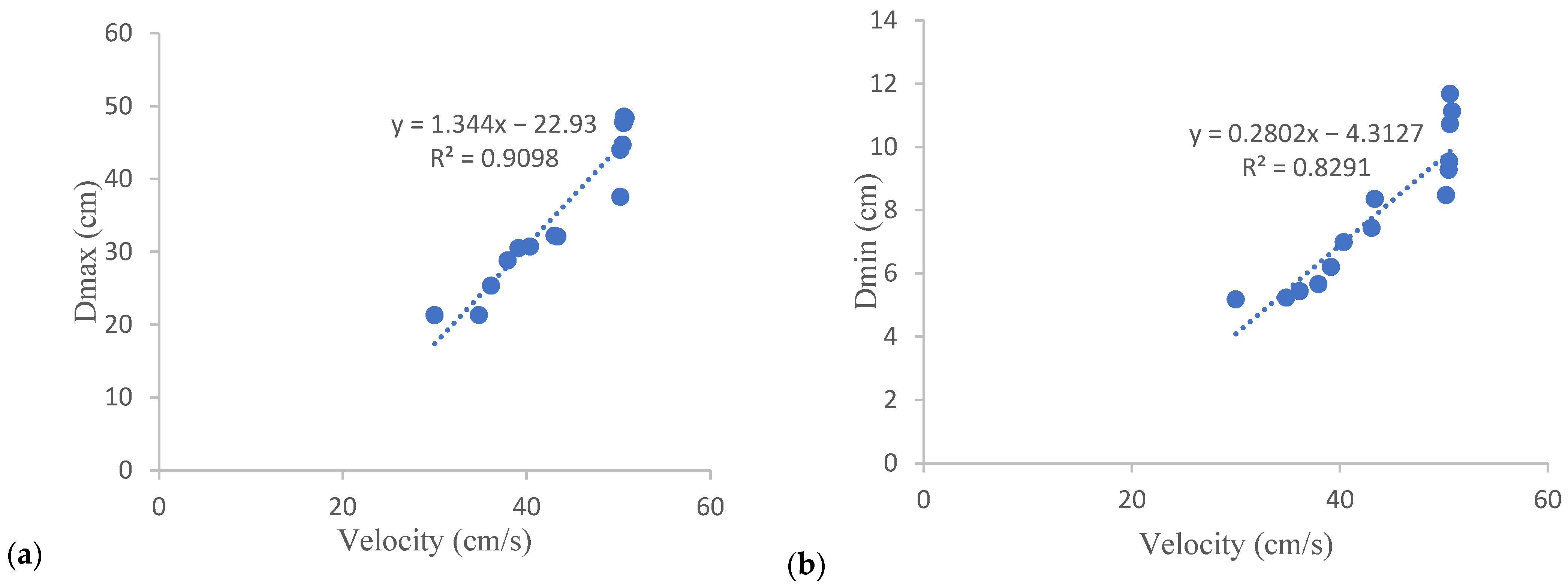
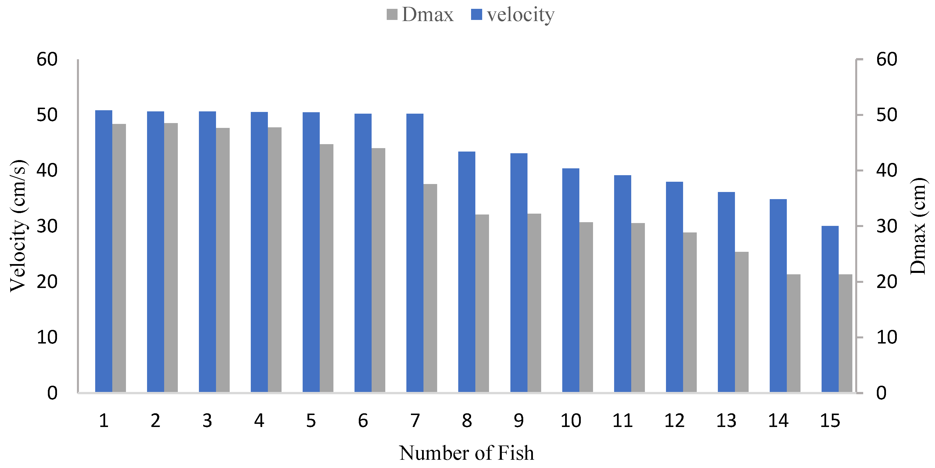
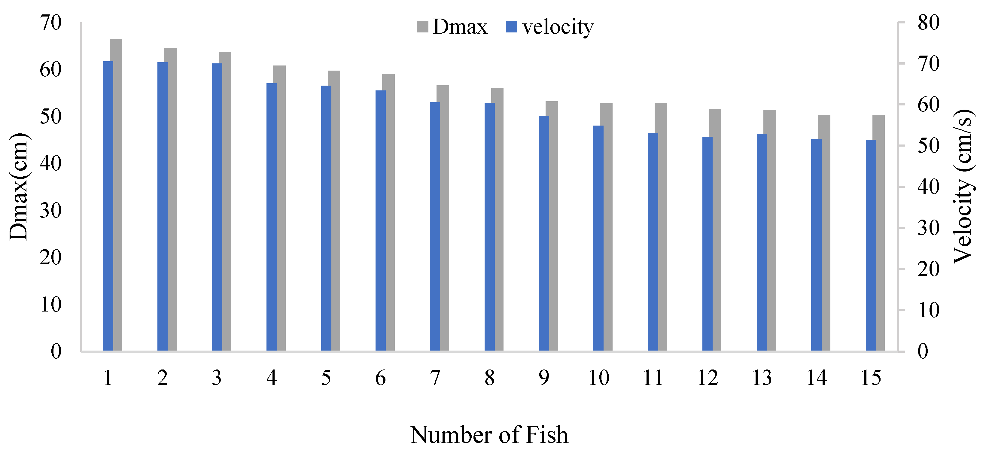
The fitting line (according to the direct and positive correlation obtained between the factors) between the speed and the measured diameters (large and small) was drawn under two normal and feeding conditions in Figure 3 and Figure 4, respectively. The R2 was equal to 0.94 and 0.89 between fish speed with large and small diameters, respectively, in normal conditions and equal to 0.92 and 0.90 in feeding conditions, respectively. Additionally, there was a linear relationship between speed and length in normal conditions and speed and small diameter in feeding conditions. There was also a quadratic relationship (quadratic function) between speed and large diameter. Additionally, the speed of fish and their maximum diameters are plotted for 15 fish to show the relationship between fish speed and maximum diameter in Figure 5 and Figure 6 under normal and feeding conditions, respectively.
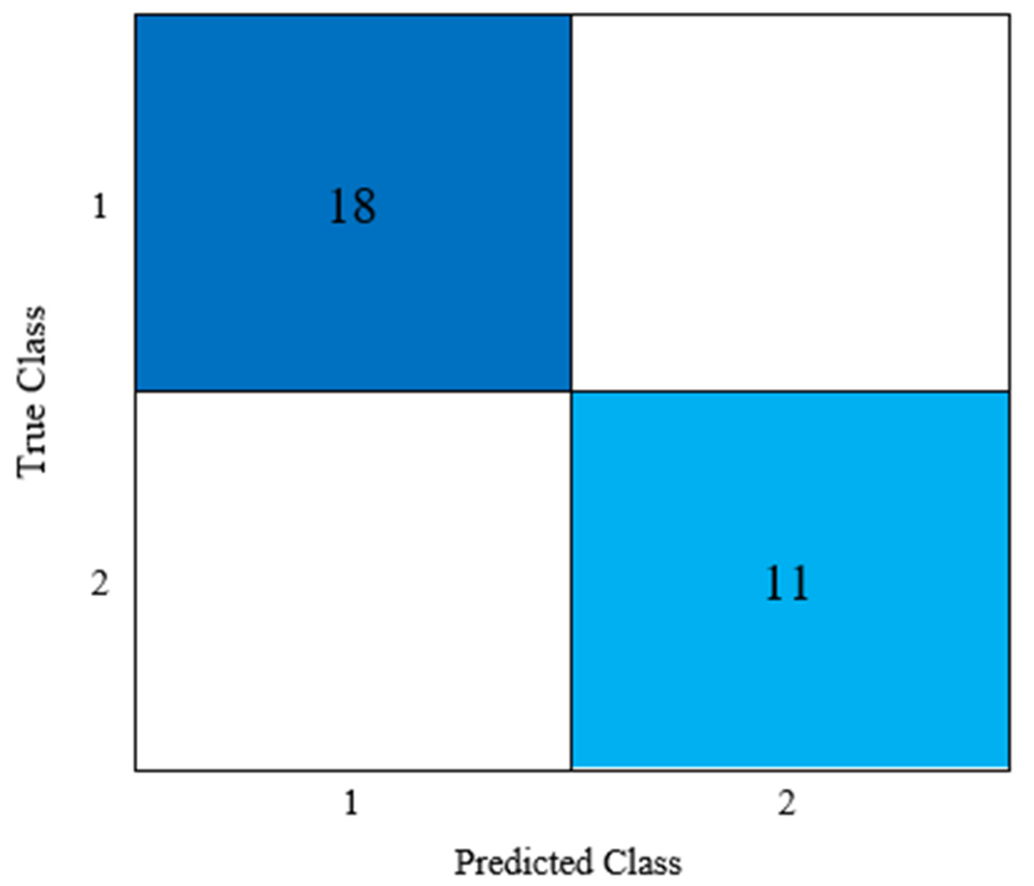
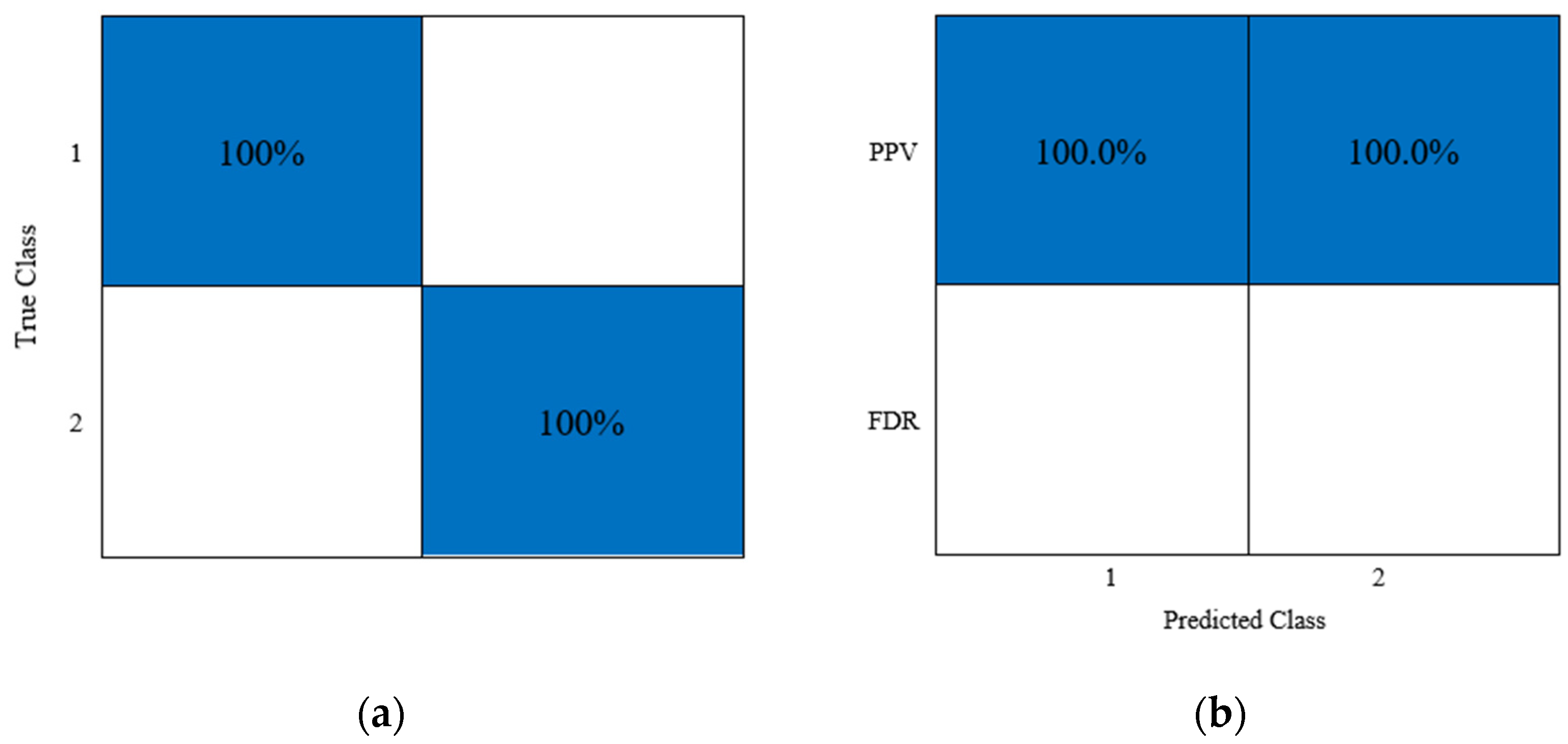
The classifier was trained under two conditions, normal and feed according to the correlation and high R2 between the large diameter and the movement speed of the samples, and then tested. In the stage of the classification test, 11 fish were detected under feeding conditions (looking for food) and 18 fish under normal conditions (Figure 7). It should be noted that the accuracy of the classification was 100% and it made the correct diagnosis based on the training it had seen (Figure 8). According to Table 4, True Positives (TP) and True Negatives (TN) are 100 percent; additionally, False Positives and False Negatives are 0 percent. Therefore, Precision, Recall, FDR, Fmeasure, and Accuracy were calculated to 100%, 100%, 0, 1, and 1%, respectively.
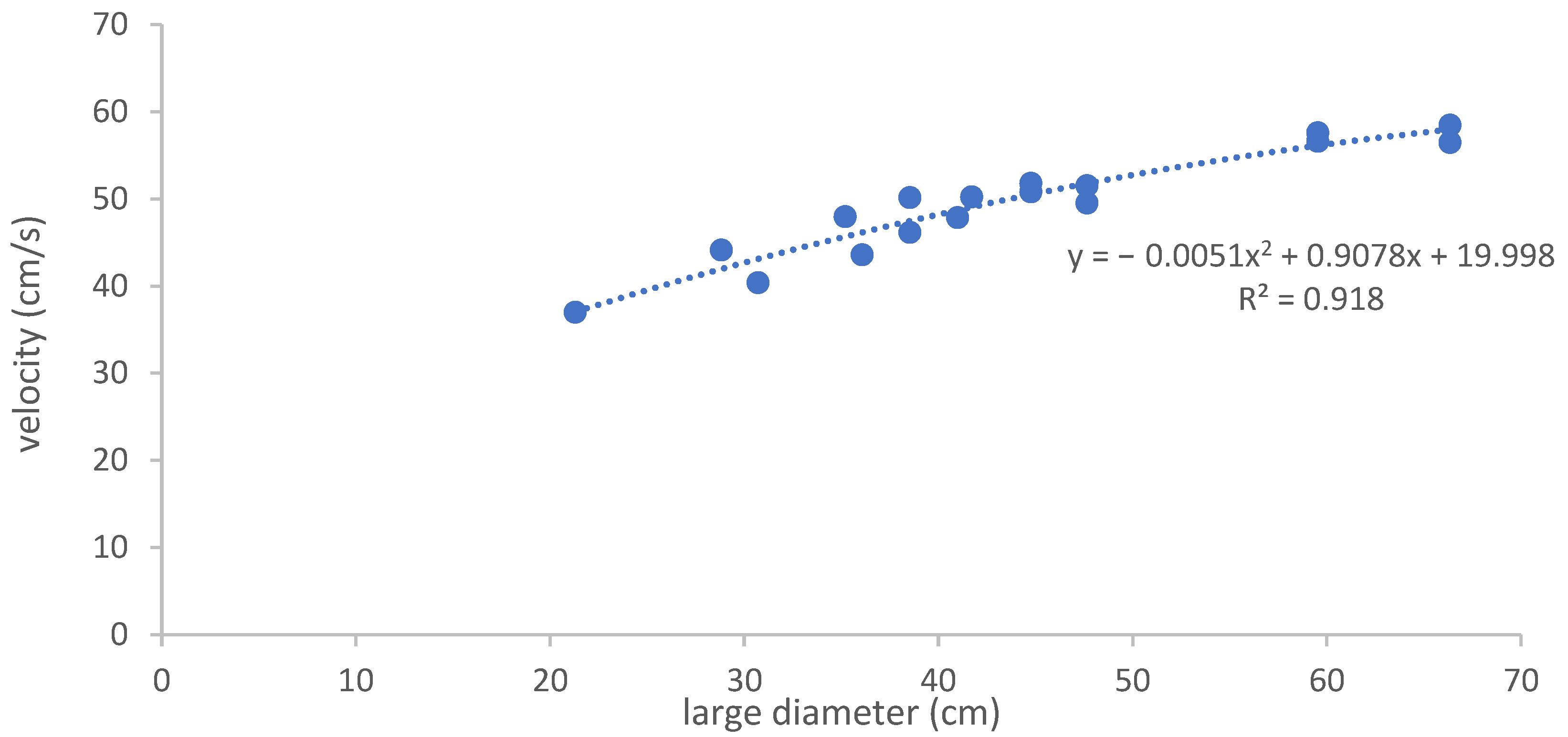
Figure 9 and Figure 10 show the fitted line drawn between the prediction of movement speed values based on the large diameter of the fish obtained by the presented system, in which the R2 is equal to 0.91 and 0.92 under two normal and feeding conditions, respectively, and there was a second-order non-linear relationship between them.

4.3. Velocity Prediction Model of Fish by Using ANN under Normal Conditions

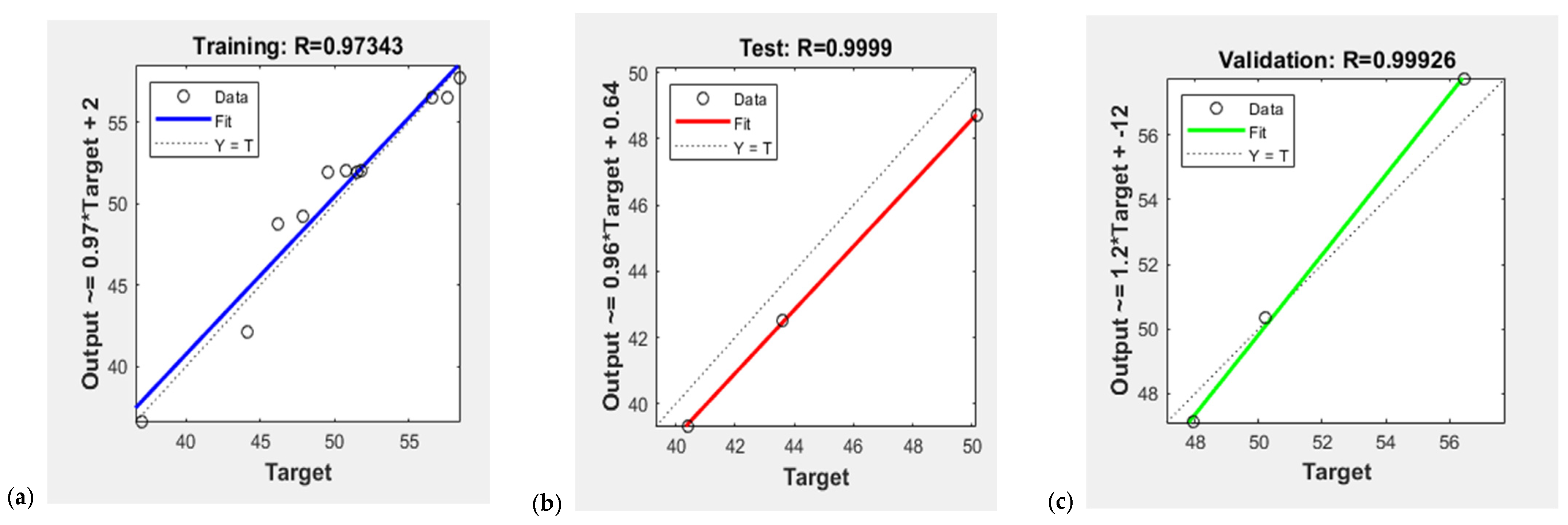
A multilayer perceptron (MLP) neural network with four inputs (Dmax, Dmin, equivalent diameter, and surface center), one hidden layer, and one output (velocity of fish) was used to predict fish speed. At first, the neural network with one to seven neurons was tested and checked, and the mean squared error (MSE) in each neuron was recorded (Table 5 and Table 6). Therefore, due to the increase in error along with the increase in the number of neurons, the training of the network with three neurons in a middle layer was chosen as the best model with the least error; so, the R2 and MSE were 0.94 0.98, and 0.98, and 1.98, 0.78, and 1.4 for train, test, and validation, respectively, in normal conditions (Table 5), and were 0.98, 0.98, and 0.98, and 0.97, 6.14, and 0.14 for train, test, and validation, respectively, in feeding conditions (Table 6). The fitting line was drawn in three stages of training, testing, and validation, as well as in general mode, to evaluate the neural network between the output of the network (predicted data related to fish velocity) and real data (measured fish velocity) (Figure 11 and Figure 12 in normal conditions and Figure 13 and Figure 14 in feeding conditions).
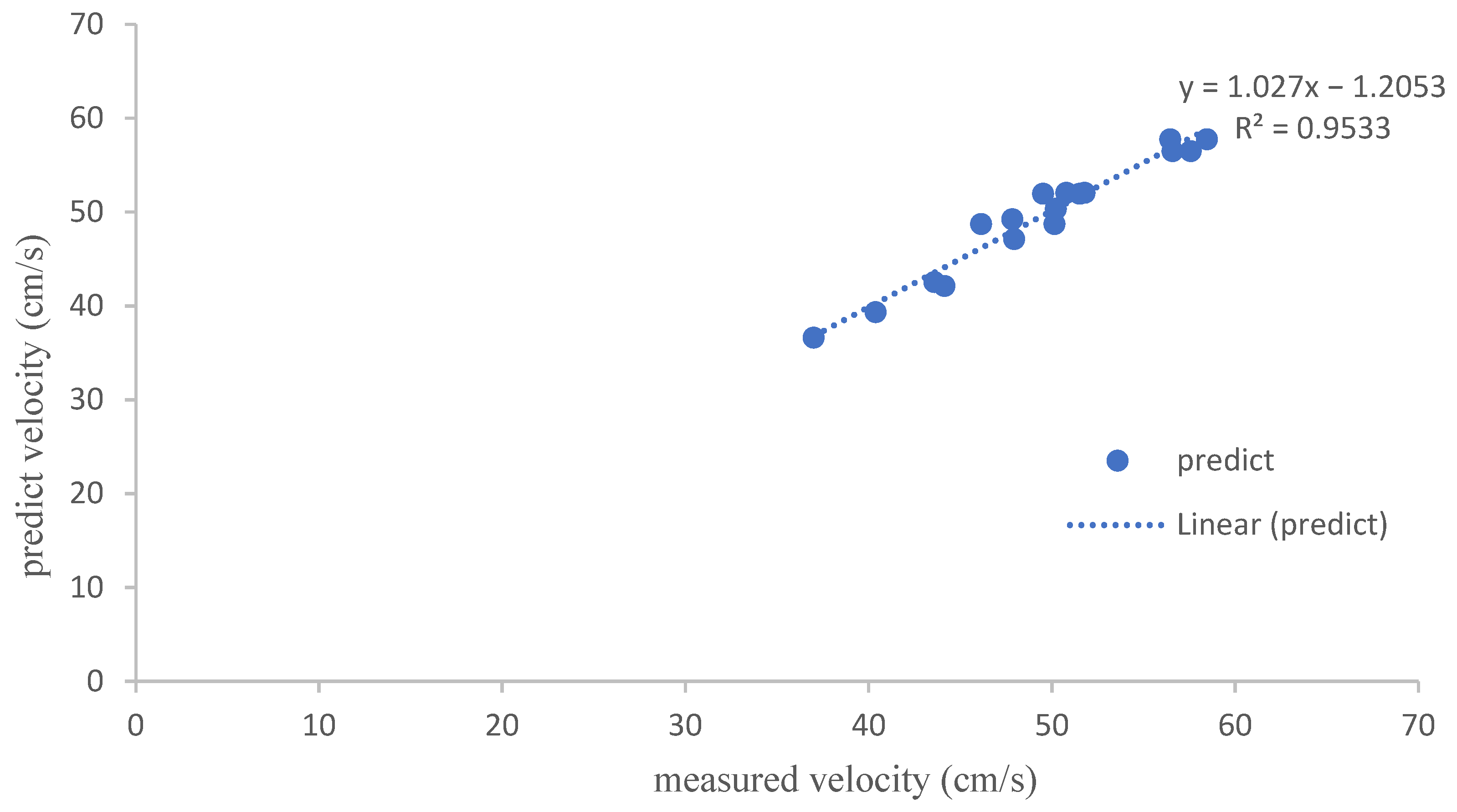
In Figure 11, the fitting line drawn is shown by the artificial neural network software between the real measured data and the predicted data in three stages of training, testing, and validation. According to the figure, the R2 in these three stages is equal to 0.97, 0.99, and 0.99, respectively. Therefore, Figure 12 shows the drawn fitting line between the actual measured speed and the predicted speed (using artificial neural network software). According to the figure, the R2 is equal to an acceptable value (0.95), which reports the high validity of the model predicted by the ANN. In the same way, the fitting line was drawn for the three stages of training, test, and validation in feeding conditions (Figure 13), where the R2 was equal to 0.99, 0.99, and 0.99, respectively. Additionally, the fitting line between the measured speed and the predicted speed using an ANN was drawn in Figure 14, which reports an acceptable validity for this model with a high R2 factor (R2 = 0.94).

4.4. Discussion

In this research, after the stage of tagging and identifying fish using YOLOv2 and classifying the images in two conditions of normal and feeding, a fitting line was drawn between the speed of movement of the fish and their body length in two conditions of normal and feeding. The R2 was equal to 0.91 and 0.92 under normal and feeding conditions, respectively. Additionally, the Precision and Accuracy were equal to 100% and 1%, respectively. In the study in [44], they used YOLO to classify objects and fish underwater and reported that this program shows a very good performance in classifying video images taken from the underwater environment. Additionally, [45] used YOLOv2 to facilitate the determination of fish freshness level (good quality, medium quality, low quality). The detection of fish freshness level for three species of fish was successfully performed, and the average Accuracy was 72.9%, the average Recall was 57.5%, and the Accuracy was 57.5%.
According to the results presented in this research and in accordance with the results of [5,35,41,46], machine vision systems or image processing methods were successfully used to investigate and distinguish fish. The application of the machine vision system and the presented classification algorithm showed high accuracy in the correct identification and separation of fish according to the speed and diameter of the fish. Additionally, according to the results of [40], the k-mean segmentation algorithm was stable and accurate and had high accuracy. To automatically detect fish in the water model, a multilayer perceptron artificial neural network with three neurons was investigated and proposed based on their maximum body diameter. According to the results, R2 was 0.97, 0.99, and 0.99 in the stages of training, testing, and validation, and an acceptable validity for the artificial neural network model was calculated with a high R2 coefficient (0.94) between the measured speed and the predicted speed.
Ref. [47] used machine vision and a new hybrid deep neural network model and proposed an automatic fish population counting method to estimate the number of Atlantic salmon, which reported an estimation accuracy of 95.06%. Ref. [48] used a region-based convolution artificial neural network to detect the free movement of fish underwater without restrictions, and the detection accuracy was 87.44% and 80.02% in the data set, respectively. Ref. [49] used artificial neural networks (ANNs) and support vector machines (SVMs) for classification to evaluate the freshness of rainbow salmon. According to the results, an ANN performed better than an SVM, so the overall classification accuracy for eye and gill color features was 84% and 96%, respectively.
However, it is suggested for future work to provide a system by imaging the pool and underwater from above to ensure economic improvement, and simultaneously measure the water and temperature parameters of the fish breeding area, as well as the growth process of the physical characteristics of the fish, such as length, color, diameter, and speed of movement. Additionally, the feeding can be performed automatically according to the examination of the characteristics of the fish, the quality of the pool water, and the conditions of the fish’s living environment, because the conditions in which the larval stages are kept have a strong influence on the growth of adult insects and thus on the quality of the final product.

5. Conclusions

The speed of movement of the fish (in response to feeding), their growth process, and other morphological characteristics are among the important factors in the health of aquaculture and also the increase in economic profit; therefore, the online and continuous monitoring of these aquatic creatures is very important in all stages of growth.
The results of the research show that the online system programmed by the artificial neural network has high efficiency and predictability for fish in both normal and feeding conditions with the least error of 1.4 and 0.14, respectively, and the highest R2 was 0.95 and 0.94, respectively, which was used with the simplest equipment, including a camera and a laptop.
This system was able to check and monitor the velocity and morphological characteristics of fishes online under both feeding and normal conditions so that if unstable conditions are detected for each of the aquatic animals, the necessary investigation can be carried out to avoid the economic damage caused by it.
In future work, we will evaluate the performance of the proposed system in additional datasets, including newly generated datasets and existing well-known datasets. This will allow us to compare our results for different species and with different growth conditions to adapt our proposal to a changing scenario similar to the real application cases. Parameters such as natural or artificial illumination, different water conditions, and the possible effect of meteorological phenomena will be included to evaluate their effect on the performance of the proposed system.

Author Contributions

Conceptualization, F.B.P.; methodology, F.B.P.; software, F.B.P. and S.A.M.; validation, F.B.P. and J.L.; formal analysis, F.B.P. and S.A.M.; investigation, F.B.P.; resources, F.B.P.; data curation, F.B.P. and S.A.M.; writing—original draft preparation, F.B.P.; writing—review and editing, F.B.P., S.A.M., L.P. and J.L.; visualization, F.B.P.; supervision, S.A.M.; project administration, J.L.; funding acquisition, L.P. All authors have read and agreed to the published version of the manuscript.

Funding

This study forms part of the ThinkInAzul program and was supported by MCIN with funding from European Union NextGenerationEU (PRTR-C17.I1) and by Generalitat Valenciana (THINKINAZUL/2021/002).

Data Availability Statement

The data presented in this study are available on request from the corresponding author. The data are not publicly available due to privacy constraints.

Acknowledgments

We would like to thank the anonymous reviewer for very helpful comments and suggestions on the manuscript.

Conflicts of Interest

The authors declare no conflict of interest.

References

  1. Akbarzadeh, A.; Karami, M.; Nezami, S.A.; Amiri, B.M.; Khara, H.; Eagderi, S. A comparative study of morphometric and meristic characters of pikeperch Sander lucioperca (L.) in Iranian waters of Caspian Sea and Aras Dam Lake. Iran. J. Biol. 2009, 22, 535–545. [Google Scholar]
  2. Amraei, S.; Mehdizadeh, S.A.; Sallary, S. Application of computer vision and support vector regression for weight prediction of live broiler chicken. Eng. Agric. Environ. Food 2017, 10, 266–271. [Google Scholar] [CrossRef]
  3. Bagheri, T.; Hedayati, A.A.; Abdoli, A. Study of some morphometric measurements, meristic traits, age and growth structure of Borbus grypus in Dalaki river. Iran Biol. Mag. 2010, 23, 389–396. [Google Scholar]
  4. Bai, Y.X.; Zhang, S.H.; Fan, Z.; Liu, X.Y.; Zhao, X.; Feng, X.-Z.; Sun, M.Z. Automatic multiple zebrafish tracking based on improved HOG features. Sci. Rep. 2018, 8, 10884. [Google Scholar] [CrossRef] [PubMed] [Green Version]
  5. Behzadi, B.; Borghei, A.M.; Javadi, A.; Minaei, S.; Almassi, M. Image Based Method to Identify Trout Fish Biometric Characteristics and Mapping Growth Curve Trout Fish by Digital Image Analysis under Laboratory Conditions. Agric. Mech. Syst. Res. 2019, 20, 113–128. [Google Scholar]
  6. Date, K.; Nagi, R. GPU-accelerated Hungarian algorithms for the linear assignment problem. Parallel Comput. 2016, 57, 52–72. [Google Scholar] [CrossRef]
  7. De Oliveira Barreiros, M.; De Oliveira Pantas, D.; De Oliveira Silva, L.C.; Ribeiro, S.; Barros, A.K. Zebrafish tracking using YOLOv2 and Kalman filter. Sci. Rep. 2021, 11, 3219. [Google Scholar] [CrossRef]
  8. Delcourt, J.; Denoël, M.; Ylieff, M.; Poncin, P. Video multitracking of fish behavior: A synthesis and future perspectives. Fish Fish. 2013, 14, 186–204. [Google Scholar] [CrossRef]
  9. Delcourt, J.; Ylieff, M.; Bolliet, V.; Poncin, P.; Bardonnet, A. Video tracking in the extreme: A new possibility for tracking nocturnal underwater transparent animals with fluorescent elastomer tags. Behav. Res. Methods 2011, 43, 590–600. [Google Scholar] [CrossRef] [Green Version]
  10. Ding, C.; Wang, S.; Liu, N.; Xu, K.; Wang, Y.; Liang, Y. REQ-YOLO: A resource-aware, efficient quantization framework for object detection on FPGAS. In Proceedings of the ACM/SIGDA International Symposium on Field-Programmable Gate Arrays, Monterey, CA, USA, 24–26 February 2019. [Google Scholar] [CrossRef]
  11. FAO. The State of World Fisheries and Aquaculture; Food and Agricultural Organization of the United Nations: Pasaden, CA, USA, 2020. [Google Scholar]
  12. Garcia, M.; Sendra, S.; Lloret, G.; Lloret, J. Monitoring and control sensor system for fish feeding in marine fish farms. IET Commun. 2010, 5, 1682–1690. [Google Scholar] [CrossRef]
  13. Garcia-Magarino, I.; Lacuesta, R.; Lloret, J. ABS-Fish count: An agent-based simulator of underwater sensors for measuring the amount of fish. Sensors 2017, 17, 2606. [Google Scholar] [CrossRef] [PubMed] [Green Version]
  14. Hassan, W.; Fore, M.; Urke, H.A.; Ulvund, J.B.; Bendiksen, E.; Alfredsen, J.A. New concept for measuring swimming speed of free-ranging fish using acoustic telemetry and Doppler analysis. Biosyst. Eng. 2022, 220, 103–113. [Google Scholar] [CrossRef]
  15. Heidari, S.; Ghaleh, E.M.; Rabbani, H.; Vesali, F. Determining of Some Water Quality Parameters in Fish Pond Using Image Processing. Iran. J. Biosyst. Eng. 2019, 50, 607–614. [Google Scholar]
  16. Hvas, M.; Oppedal, F. Sustained swimming capacity of Atlantic salmon. Aquac. Environ. Interact. 2017, 9, 361–369. [Google Scholar] [CrossRef] [Green Version]
  17. Hvas, M.; Folkedal, O.; Solstorm, D.; Vågseth, T.; Fosse, J.O.; Gansel, L.C.; Oppedal, F. Assessing swimming capacity and schooling behaviour in farmed Atlantic salmon Salmo salar with experimental push-cages. Aquaculture 2017, 473, 423–429. [Google Scholar] [CrossRef] [Green Version]
  18. Izgi, E.; Oztopal, A.; Yerli, B.; Kaymak, M.K.; Sahin, A.D. Short-mid-term solar power prediction by using artificial neural networks. J. Int. Sol. Energy 2012, 86, 725–733. [Google Scholar] [CrossRef]
  19. Jeong, S.J.; Yang, Y.S.; Lee, K.; Kang, J.G.; Lee, D.G. Vision-based automatic system for non-contact measurementof morphometric characteristics of flatfish. J. Electr. Eng. Technol. 2013, 8, 1194–1201. [Google Scholar] [CrossRef] [Green Version]
  20. Mirat, O.; Sternberg, J.R.; Severi, K.E.; Wyart, C. Zebra Zoom: An automated program for high-throughput behavioral analysis and categorization. Front. Neural Circuits 2013, 7, 107. [Google Scholar] [CrossRef] [Green Version]
  21. Mirhaji, H.; Soleymani, M.; Asakereh, A.; Mehdizadeh, S.A. Fruit détection and load estimation of an orange orchard using the YOLO models through simple approches in different Imaging and illumination conditions. Comput. Electron. Agric. 2021, 191, 106533. [Google Scholar] [CrossRef]
  22. Moreno, A.; Gilabert, M.A.; Martinez, B. Mapping daily global solar irradiation over Spain: A comparative study of selected approaches. J. Int. Sol. Energy 2011, 85, 2072–2084. [Google Scholar] [CrossRef]
  23. Parra, L.; Sendra, S.; Garcia, L.; Lloret, J. Design and deployment of low-cost sensors for monitoring the water quality and fish behavior in aquaculture tanks during the feeding process. Sensors 2018, 18, 750. [Google Scholar] [CrossRef] [PubMed] [Green Version]
  24. Pérez-Escudero, A.; Vicente-Page, J.; Hinz, R.C.; Arganda, S.; de Polavieja, G.G. idTracker: Tracking individuals in a group by automatic identification of unmarked animals. Nat. Methods 2014, 11, 743–748. [Google Scholar] [CrossRef]
  25. Pourmozaffar, S.; Jabaleh, A.; Safiyari, H.; Rameshi, H.; Jahromi, S.T.; Gozari, M.; Zahedi, M. Evaluation of Morphometric changes of rainbow Trout (Oncorhynchus mykiss) using image processing method (IPM). Ecol. Water Resour. J. 2019, 4, 28–35. [Google Scholar]
  26. Qian, Z.-M.; Cheng, X.E.; Chen, Y.Q. Automatically detect and track multiple fish swimming in shallow water with frequent occlusion. PLoS ONE 2014, 9, e106506. [Google Scholar] [CrossRef] [PubMed] [Green Version]
  27. Redmon, J.; Farhadi, A. YOLO9000: Better, faster, stronger. In Proceedings of the IEEE Conference on Computer Vision and Pattern Recognition (CVPR), Honolulu, HI, USA, 21–26 July 2017; pp. 6517–6525. [Google Scholar]
  28. Remen, M.; Solstorm, F.; Bui, S.; Pascal, K.; Vagseth, T.; Solstorm, D.; Hvas, M.; Oppedal, F. Critical swimming speed in groups of Atlantic salmon Salmo salar. Aquac. Environ. Interact. 2016, 8, 659–664. [Google Scholar] [CrossRef] [Green Version]
  29. Siriani, A.L.R.; Kodaira, V.; Mehdizadeh, S.A.; De Alencar Nass, I.; de Moura, D.J.; Pereira, D.F. Detection and tracking of chickens in low-light images using YOLO network and Kalman filter. Neural Comput. Appl. 2022, 34, 21987–21997. [Google Scholar] [CrossRef]
  30. Romero-Ferrero, F.; Bergomi, M.G.; Hinz, R.C.; Heras, F.J.H.; de Polavieja, G.G. Idtracker.ai: Tracking all individuals in small or large collectives of unmarked animals. Nat. Methods 2019, 16, 179–182. [Google Scholar] [CrossRef] [PubMed]
  31. Safiyari, H.; Jafari, A.; Raoufat, M.H.; Nassiri, S.M. Feasibility of sorting the tigertooth croaker (Otolithes ruber) and silver pomfret (Pampus argenteus) fishes using computer vision technology. J. Fish. (Iran. J. Nat. Resour.) 2015, 68, 267–286. [Google Scholar]
  32. Sanuade, O.A.; Hassan, A.M.; Akanji, A.O.; Olaojo, A.A.; Oladunjoye, M.A.; Abdulraheem, A. New empirical equation to estimate the soil moisture content based on thermal properties using machine learning techniques. Arab. J. Geosci. 2020, 13, 377. [Google Scholar] [CrossRef]
  33. Sarkar, U.K.; Khan, G.E.; Dabas, A.; Pathak, A.K.; Mir, J.I.; Rebello, S.C.; Pal, A.; Singh, S.P. Length-weight relationship and condition factor of selected freshwater fish species found in river Ganga, Gomti and Rapti, India. J. Environ. Biol. 2013, 34, 951–956. [Google Scholar]
  34. Singh, L.; Alam, A.; Kumar, V.K.; Kumar, D.; Kumar, P.; Jaffery, Z.A. Design of thermal imaging-based health condition monitoring and early fault detection technique for porcelain insulators using Machine learning. Environ. Technol. Innov. 2021, 24, 102000. [Google Scholar] [CrossRef]
  35. Torisawa, S.; Kadota, M.; Komeyama, K.; Suzuki, K.; Takagi, T. A digital stereo-video camera system for three-dimensional monitoring of free-swimming Pacific bluefin tuna, Thunnus orientalis, cultured in a net cage. Aquat. Living Resour. 2011, 24, 107–112. [Google Scholar] [CrossRef] [Green Version]
  36. Turan, C. A note on the examination of morphometric differentiation among fish populations: The truss system. Turk. J. Zool. 1999, 23, 259–264. [Google Scholar]
  37. Velayatzadeh, M.; Hamidinejad, M. Importance and position of Indian carp grove in the Iranian fishery industry. First Aquat. Sci. Conf. 2012, 50, 272–276. (In Farsi) [Google Scholar]
  38. Wang, S.H.; Cheng, X.E.; Qian, Z.-M.; Liu, Y.; Chen, Y.Q. Automated planar tracking the waving bodies of multiple zebrafish swimming in shallow water. PLoS ONE 2016, 11, e0154714. [Google Scholar] [CrossRef] [Green Version]
  39. Wang, X.; Cheng, E.; Burnett, I.S.; Wilkinson, R.; Lech, M. Automatic tracking of multiple zebrafish larvae with resilience against segmentation errors. In Proceedings of the IEEE 15th International Symposium on Biomedical Imaging (ISBI 2018), Washington, DC, USA, 4–7 April 2018; pp. 1157–1160. [Google Scholar] [CrossRef]
  40. Yao, H.; Duan, Q.; Li, D.; Wang, J. An improved K-means clustering algorithm for fish image segmentation. Math. Comput. Model. 2013, 58, 790–798. [Google Scholar] [CrossRef]
  41. Zabihi, J.; Nassiri, M.; Jafari, A.A. Estimation of density of trout in fish farm using image processing technique. J. Fish. (Iran. J. Nat. Resour.) 2014, 67, 49–59. [Google Scholar]
  42. Zhang, L.; Wang, J.; Duan, Q. Downscaling groundwater storage data in China to a 1-km resolution using machine learning methods. Remote Sens. 2020, 13, 523. [Google Scholar] [CrossRef]
  43. Xu, Z.; Cheng, X.E. Zebrafish tracking using convolutional neural networks. Sci. Rep. 2017, 7, 42815. [Google Scholar] [CrossRef] [Green Version]
  44. Park, J.H.; Kang, C. A study on enhancement of fish recognition using cumulative mean of Yolo network in underwater video images. J. Mar. Sci. Eng. 2020, 8, 952. [Google Scholar] [CrossRef]
  45. Anas, D.F.; Jaya, I.; Nurjanah. Designed and implementation of fish freshness detection algorithm using deep learning. IOP Conf. Ser. Earth Environ. Sci. 2021, 944, 012007. [Google Scholar] [CrossRef]
  46. Zion, B.; Ostrovsky, V.; Karplus, I.; Lidor, G.; Barki, A. Ornamental Fish Mass Estimation by Image Processing; Agricultural Research Organization: Bet Dagan, Israel, 2012. [Google Scholar]
  47. Zhang, T.; Xu, C.; Yang, M.-H. Multi-task correlation particle filter for robust object tracking. In Proceedings of the IEEE Conference on Computer Vision and Pattern Recognition (CVPR), Honolulu, HI, USA, 21–26 July 2017; pp. 4819–4827. [Google Scholar]
  48. Salman, A.; Siddiqui, S.A.; Shafait, F.; Mian, A.; Shortis, M.R.; Khurshid, K.; Ulges, A.; Schwanecke, U. Automatic fish detection in underwater videos by a deep neural network-based hybrid motion learning system. Int. Counc. Explor. Sea (ICES) J. Mar. Sci. 2020, 77, 1295–1307. [Google Scholar] [CrossRef]
  49. Lalabadi, H.M.; Sadeghi, M.; Mireei, S.A. Fish freshness categorization from eyes and gills color feature using multi class artificial neural network and support vector machines. Agric. Eng. 2020, 90, 102076. [Google Scholar]
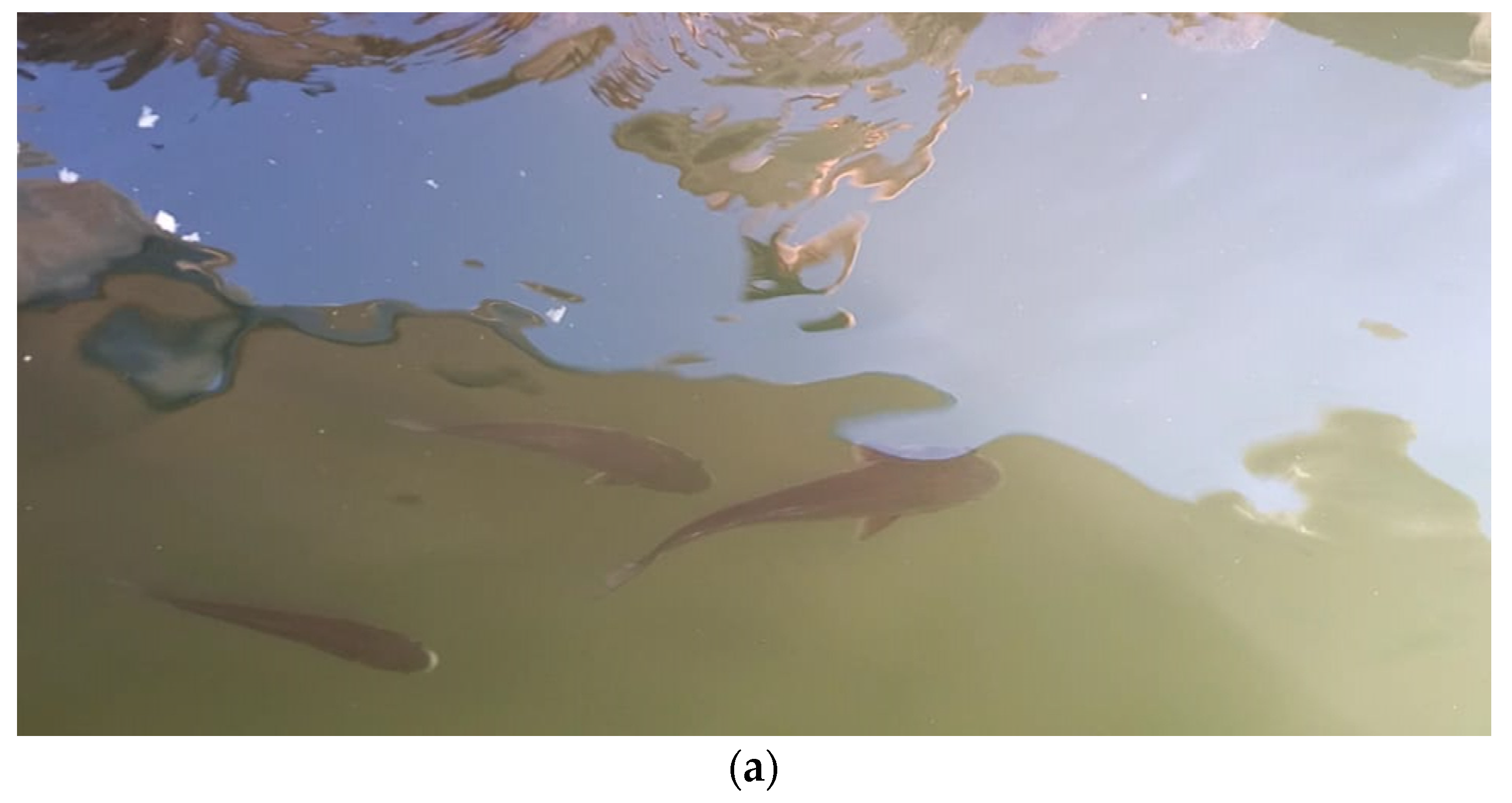
Figure 1. An image of fish tracked and labeled in MATLAB program. (a) Several fish in place of data collection. (b) Tracking of fish using MATLAB software.
Water 15 02138 g001aWater 15 02138 g001b
Figure 2. Schematic of the system installed for online fish monitoring. (1) Camera. (2) Laptop. (3) Wifi. (4) Fish.
Water 15 02138 g002
Figure 3. The fitted line drawn between the velocity and the diameter of the fish under normal conditions: (a) max diameter; (b) min diameter.
Water 15 02138 g003
Figure 4. The fitted line drawn between the velocity and the diameter of the fish under feeding conditions: (a) max diameter; (b) min diameter.
Water 15 02138 g004
Figure 5. The relation between velocity (cm/s) and max diameter of fish under normal conditions.
Water 15 02138 g005
Figure 6. The relation between velocity (cm/s) and max diameter of fish under feeding conditions.
Water 15 02138 g006
Figure 7. Classification diagnosis: the 11 fish in feeding conditions (seeking food) and 18 fish in normal conditions.
Water 15 02138 g007
Figure 8. (a) The classification accuracy in distinguishing two groups of fish (under normal and feeding conditions); (b) the classification of PPV and FDR.
Water 15 02138 g008
Figure 9. The fitted line drawn between velocity values predicted by the system and the large diameters of the fish under normal conditions.
Water 15 02138 g009
Figure 10. The fitted line drawn between the velocity and the large diameter of the fish under feeding conditions.
Water 15 02138 g010
Figure 11. The fitting line between the real velocity of fish and the predicted velocity using an ANN in train, test and validation steps in normal conditions; (a) Training level (b) Test level (c) Validation level.
Water 15 02138 g011
Figure 12. The fitting line between the real velocity of fish and the predicted velocity using an ANN in normal conditions.
Water 15 02138 g012
Figure 13. The fitting line between the real velocity of fish and the predicted velocity using an ANN in train, test, and validation steps in feeding conditions; (a) Training level (b) Test level (c) Validation level.
Water 15 02138 g013
Figure 14. The fitting line between the real velocity of fish and the predicted velocity using an ANN in feeding conditions.
Water 15 02138 g014
Table 1. Analysis of variance velocity and the maximum diameter under two conditions of normal and feeding.
CorrelationtdfStd. Error
Velocity (normal) and velocity (feeding)0.91 **−20.71 **140.76
Dmax (normal) and Dmax (feeding)0.95 **−15.75 **141.3
Note(s): **, is significance of 5%.
Table 2. Correlation between velocity and large diameter, small diameter, surface center, and equivalent diameter in normal conditions.
Max DiameterMin DiameterVelocitySurface CenterEquivalent Diameter
Max diameter1
Min diameter0.89 **1
Velocity0.92 **0.84 **1
Surface center0.85 **0.98 **0.82 **1
Equivalent diameter0.90 **0.96 **0.85 **0.99 **1
Note(s): ** Correlation is significant at the 0.01 level (2-tailed).
Table 3. Correlation between velocity and large diameter, small diameter, surface center, and equivalent diameter in feeding conditions.
Max DiameterMin DiameterVelocitySurface CenterEquivalent Diameter
Max diameter1
Min diameter0.97 **1
Velocity0.98 *0.95 **1
Surface center0.93 **0.98 **0.91 **1
Equivalent diameter0.96 **0.97 **0.94 **0.96 **1
Note(s):*, ** Correlation is significant at the 0.01 and 0.05 level (2-tailed).
Table 4. Evaluation of the proposed diagnosis model based on Precision, sensitivity (Recall), FDR, error (Fmeasure), and Accuracy.
True Positives (TP) (%)True Negatives (TN) (%)False Positives (FP) (%)False Negatives (FN) (%)
10010000
Precision T P T P + F P × 100 = 100 %
Recall T P T P + F N × 100 = 100 %
FDR F P T P + F P = 0
Fmeasure 2 × ( P r e c i s i o n × R e c a l l ) P r e c i s i o n + R e c a l l = 1
Accuracy T P + T N T P + F P + F N + T N × 100 = 1
Table 5. The results of the artificial neural network from 1 to 7 neurons in the stages of training, testing, and validation, and presenting the MSE and R2 in normal conditions.
The Number of NeuronsEvaluationRMSER2
Train0.980.660.96
1Test0.995.290.98
Validation0.990.720.98
Train0.972.680.94
2Test0.992.840.98
Validation0.892.550.79
Train0.971.980.94
3Test0.990.780.98
Validation0.991.40.98
Train0.897.930.79
4Test0.990.270.98
Validation0.983.70.96
Train0.980.700.96
5Test0.9014.40.81
Validation0.990.450.98
Train0.980.480.96
6Test0.967.250.92
Validation0.9913.550.98
Train0.990.390.98
7Test0.954.590.90
Validation−0.052.800.0025
Table 6. The results of the artificial neural network from 1 to 7 neurons in the stages of training, testing, and validation, and presenting the MSE and R2 in feeding conditions.
The Number of NeuronsEvaluationR-ValidationMSER2
Train0.9715.040.94
1Test0.9818.470.96
Validation0.992.520.98
Train0.972.830.94
2Test0.9810.970.96
Validation086.190
Train0.990.970.98
3Test0.996.140.98
Validation0.990.140.98
Train0.8238.320.67
4Test0.9810.530.96
Validation0.9910.98
Train0.7223.030.51
5Test0.987.690.96
Validation0.9921.090.98
Train0.6345.810.39
6Test0.9854.280.96
Validation0.994.300.98
Train0.990.690.98
7Test0.995.430.98
Validation0.98127.410.96
Disclaimer/Publisher’s Note: The statements, opinions and data contained in all publications are solely those of the individual author(s) and contributor(s) and not of MDPI and/or the editor(s). MDPI and/or the editor(s) disclaim responsibility for any injury to people or property resulting from any ideas, methods, instructions or products referred to in the content.