Research on Seismic Connectivity Reliability Analysis of Water Distribution System Based on CUDA

Abstract

To improve the seismic connectivity reliability (SCR) analysis efficiency of water distribution systems (WDS) based on Monte Carlo (MC) simulation, the quasi-Monte Carlo (QMC) method sampled by a low-discrepancy sequence is applied. Furthermore, a parallel algorithm combined with the breadth-first search algorithm for SCR analysis of WDS based on the QMC method and Compute Unified Device Architecture (CUDA) platform was proposed. A city WDS was taken as a computational example, the accuracy and efficiency of the traditional MC algorithm and parallel algorithm were compared, and the influence of the Sobol sequence and pseudo-random number sequence was analysed. The analysis results show that when 1,000,000 simulations are performed, the maximum error of the calculation results of the two methods is 0.2%, and the parallel method can obtain a six-fold speedup ratio compared with the serial method, indicating that the proposed parallel method is correct, meets the accuracy requirements, and helps to improve the SCR analysis efficiency. When the number of simulations is the same, the simulation results based on the Sobol sequence are more accurate than those based on the pseudo-random number sequence. The proposed parallel method also achieves a good acceleration effect in the SCR analysis of large-scale WDS.

1. Introduction

Urban water supply systems, gas supply systems, power supply systems and other infrastructure systems are the lifeblood to maintain the economic and social functions of the city, and people call them lifeline projects. With the rapid development of the national economy, the scale of the city increases, the degree of modernisation is increasingly high, and the dependence on the lifeline project is increasingly strong. However, in increasingly frequent natural disasters, especially under the action of a strong earthquake [1,2,3], lifeline projects suffered serious damage, and water supply, power supply, communication and other services were interrupted, which caused secondary disasters, and even led to paralysis of the function of the whole city, resulting in a large number of life and property losses.

The water distribution system (WDS) is an indispensable infrastructure in urban lifeline projects, with the characteristics of wide spatial distribution and strong damage correlation, which has been severely damaged in previous destructive earthquakes, resulting in partial or complete failure of the urban water supply function and seriously affecting people’s lives [4,5,6,7,8,9]. Therefore, it is necessary to carry out seismic connectivity reliability (SCR) analysis to understand the ability of a WDS to perform its function in the first instance and provide scientific support for the pre-earthquake reinforcement and post-earthquake reconstruction of a WDS, and as a preliminary analysis of the water network resilience. The SCR analysis of a WDS involves researching its seismic reliability at the system level and analysing the connection probability between user nodes and water sources [10,11,12].

The existing reliability analysis methods include the probability theory method [13,14,15,16], boundary approximation method [17,18,19,20] and random simulation method [10,21,22]. The probability theory method includes the conditional probability method, connected set method, and cut set method, which can be utilised to solve the exact solution of connection reliability problem of a WDS. However, when the WDS is too complex and involves too many pipelines and nodes, it will generate a huge amount of work, which limits the application and development of the method. The boundary approximation method is utilised to calculate the upper and lower limits of system reliability and specify the upper and lower limit difference value to obtain the approximate solution of pipe network system reliability. The research focus of this kind of method is to find efficient methods to solve the upper and lower limit values, including the Dotson method, the M-Dotson method, and the minimal cut-based recursive decomposition algorithm. The principle of the random simulation method is the law of large numbers and Bernoulli’s principle in probability theory [23]. It holds that when the number of tests is large enough, the occurrence frequency of an event is equal to its probability of occurrence. The simulation error of the random simulation method is proportional to the sampling variance and inversely proportional to the square of the simulation sampling times.

Compared with the probability theory method and boundary approximation method, the random simulation method has great advantages in the reliability analysis of large complex networks because it avoids NP-hard problems in network reliability analysis, is insensitive to the dimensions of problems, does not need to consider the complexity of network topology, and is convenient for modelling. Its disadvantages are also obvious: it must be repeated operations to obtain more accurate and stable results, which often take a long time to calculate, its simulation time is proportional to the scale of the network diagram and the number of simulations, and the error is inversely proportional to the number of simulations. The random simulation method belongs to the statistical test method, including the Monte Carlo (MC) [24,25] method and quasi-Monte Carlo (QMC) [26] method. The MC method is widely used in the seismic reliability evaluation of WDS [21,27,28]. To improve the computational efficiency of MC, various variance reduction techniques have been studied, such as the control variable method [29], the stratified sampling method [30], and the important sampling method [31]. Those methods all use pseudorandom numbers when sampling system components. From the perspective of individual sampling points, they all follow the same probability distribution. However, from the perspective of the collection of sampling points as a whole, there will be clusters of local sampling points and sparse sampling points in the sampling space, which makes the sampling points unable to cover the whole sampling space well. To solve this problem, the QMC method changes the sampling approach and adopts a deterministic low discrepancy sequence (LDS) for sampling. Compared with the pseudo-random number sequence, LDS has better uniformity, which makes the calculation results of QMC have higher error accuracy. Its initial application can be seen in the research fields of security pricing [32], structural reliability evaluation [33] and statistical circuit analysis [34], however, it still has relatively less application in the WDS field.

With the rapid advance of the Graphics Processing Unit (GPU) [35] and the advent of Computer Unified Device Architecture (CUDA) [36], GPU parallel computing technology based on the CUDA platform has been widely used. CUDA is a parallel computing platform and programming model developed by NVIDIA for general-purpose computing graphics processing units. Developers can take advantage of the powerful parallel computing engine of graphic processing units (GPUs) to speed up their programs through CUDA. In GPU-accelerated applications, the computationally complex and logically strong part runs on the Central Processing Units (CPU), while the computationally intensive, logically simple, and data-decoupling part is processed on the GPU. Since the results produced by the random simulation method are independent each time, it has natural parallelism and is very suitable for parallel computing. Some scholars have carried out parallel research on simulation methods using GPU technology in their respective fields and achieved good acceleration effects [37,38,39,40]. Therefore, GPU technology can also be applied to SCR analysis of WDS.

At present, research on SCR analysis of WDS is quite mature. However, with the continuous progress of urbanisation, the scale of the urban WDS is increasing. How to improve the efficiency of SCR analysis of WDS is the focus of current research. In the present paper, combining graph theory and the QMC simulation technique, an efficient method for the SCR analysis of WDS is proposed. Furthermore, a CUDA-based parallel algorithm is developed to further improve the SCR analysis efficiency of WDS.

2. Graph Theory

Graph theory is a branch of mathematics that deals with graphs [41]. A graph is composed of a set of vertices and a set of binary relations between vertices. It is often used to describe a specific relationship between things, where vertices represent things and edges represent the relationship between corresponding things. Actually, it is an important data structure that can appropriately describe or model problems in many areas of the natural and social sciences. To use a computer program to analyse and study a graph, the graph must be stored in some form in the computer memory. There are many ways to store graphs on a computer, including the adjacency matrix [42], incidence matrix [43], and adjacency list [44]. The WDS is a complex network system composed of water supply sources (water plants, water wells, highland pools, etc.), nodes (concentrated water points, user demand terminals, etc.), and pipelines. In essence, it can be simplified as a network topology composed of points and edges, and its mathematical model can be represented by a graph. It should be noted that in a WDS the flow in the pipe could be unidirectional or bi-directional, thus the WDS can be abstracted as a directed graph.

3. Application of the QMC Method in SCR Analysis of WDS

3.1. QMC Method Principle

The basic idea of the QMC method [10,45] is to establish a probabilistic model or stochastic process related to the solution of the problem, whose parameters are equal to the solution of the problem; then, the statistical characteristics of the desired parameters are calculated through the observation or sampling test of the probability model or random process; finally, the approximate solution of the problem is given according to the requirements of solution accuracy or test times. Compared with the traditional MC method, the key of the QMC method is to use LDS to sample and simulate the problem. For example, when the QMC method is used to solve the integral on the unit hypercube I^s = [0, 1]^s, the calculation formula can be written as follows:

$${\displaystyle {\int }_{I^s}f\left(x\right)dx}\approx \frac{1}{N}{\displaystyle \sum _{k=1}^{N}f\left(x_k\right)}$$

(1)

where N is the number of sampling times, x_k is the random of the kth sampling and x = {x₁, x₂, …, x_N} is LDS. According to the Koksma–Hlawka inequality, the order of the error of the QMC integral can be obtained as follows:

$$\left.\left|{\displaystyle {\int }_{I^s}f\left(x\right)dx}-\frac{\mathrm{1}}{N}{\displaystyle \sum _{k=1}^{N}f\left(x_k\right)}\right.\right|\le V(F)D_N^{\ast }(x_1,\dots ,x_N)$$

(2)

where D_N* is the discrepancy degree of the LDS, which can be defined as follows:

$$D_N^{\ast }=\underset{V\subset I^s}{\sup }\left|\left.\frac{U(x_{\mathrm{1}},x_{\mathrm{2}},\dots ,x_N)}{N}-\lambda (V)\right|\right.$$

(3)

where V is any hypercube contained in I^s, U (x₁, x₂, …, x_n) is the number of points in LDS{x₁, x₂, …, x_N} contained in region V, and λ(V) is the Lebesgue measure of region V.

Equation (2) gives the upper limit of the integral error of the QMC method, indicating that the smaller the discrepancy degree of the sequence used is, the more accurate the result of integration. For an LDS containing N points, the discrepancy degree of the sequence is O(N⁻¹(logN)^s−1), and the order of the error convergence rate using the QMC method is O(N⁻¹). However, the order of the error convergence rate using the MC method is O(N^−1/2), which shows that the calculation result of the QMC method has higher accuracy than that of the MC method when the same sampling times are sampled [46].

3.2. Sobol Sequence

The construction of the LDS is the key content of the QMC method. The advantage of the LDS is that the samples generated tend to be more evenly distributed. At present, the commonly used LDS include the Halton sequence [47], Sobol sequence [48] and Latin hypercube sequence [49]. In this study, the Sobol sequence is used to sample the failure probability of WDS pipelines. The construction method of the Sobol sequence is briefly introduced below.

Suppose m_i is a positive odd number less than 2ⁱ, then the direction number d_i is calculated as follows:

d_i = m_i/2ⁱ (i=1,2,…w)

(4)

where w is the number of direction numbers; d_i is generated by a simple polynomial, which can be expressed as follows:

$$f(x)=x^q+a_1{x}^q{}^{-1}+a_2{x}^q{}^{-2}+\cdots +a_{q-1}x+1$$

(5)

where a_q equals 0 or 1. When i > q, d_i can be expressed by the following recursive formula:

$$d_i=a_1{d}_{i-1}\oplus a_2{d}_{i-2}\oplus \cdots \oplus a_q{d}_{i-q}\oplus [d_{i-q}/2^q]$$

(6)

where ⊕ represents the bitwise XOR of the binary system. For example, 0 ⊕ 1 = 1 ⊕ 0 = 1, 1 ⊕ 1 = 0 ⊕ 0 = 0.

For m_i, the equivalent recurrence formula is expressed as follows:

$$m_i=2a_1{m}_{i-1}\oplus 2^2{a}_2{m}_{i-2}\oplus \cdots \oplus 2^q{a}_q{m}_{i-q}\oplus m_{i-q}$$

(7)

Then the kth number in the Sobol sequence is generated as follows:

$$r_k=c_1{d}_1\oplus c_2{d}_2\oplus c_3{d}_3\oplus \cdots$$

(8)

where ($\cdots$c₃c₂c₁) is the binary representation of k.

To improve the generation speed of Sobol sequences, Antonov and Saleev proposed an improved calculation method [50], which uses the following recursive:

$$r_k=g_0(k)d_1\oplus g_1(k)d_2\oplus g_2(k)d_3\oplus \cdots \oplus g_{n-1}(k)d_n$$

(9)

$$r_{k+1}=r_k\oplus d_j$$

(10)

where $\cdots$g₂(k)g₁(k)g₀(k) is a binary representation of gray code with a variable k − 1. j is equal to the smallest n that satisfies g_n(k) = 0.

Figure 1a,b show the two-dimensional distribution of the pseudo-random sequence and Sobol sequence sampled 2000 times in the range of 0 to 1, respectively. It can be seen that the sampling points of the pseudo-random sequence are prone to local clustering, while the Sobol sequence has better uniformity than the pseudo-random sequence.

3.3. SCR Analysis of WDS Based on the QMC Method

The basic idea of using the QMC method to analyse the SCR of a WDS is to generate a large number of quasi-random numbers and compare them with the failure probability of pipelines to determine the failure state of each pipeline in the WDS. In each simulation, the connectivity between the water supply source and demand nodes is judged. Then, the frequency of each node in the connected state after multiple simulations is calculated, and the probability evaluation of its connectivity reliability is obtained.

When analysing the SCR of a WDS, it is ordinarily assumed that the water supply source and demand nodes will not be damaged under earthquake action. Without considering the change in water pressure at the node after the earthquake, the water in the pipe always flows from the high hydraulic pressure side to the low hydraulic pressure side. In this case, there is only one unique path between two nodes. Consequently, the topology of the WDS can be abstracted as a directed graph with edge weights. In this article, an adjacency table is used as the storage method of the pipe network, and the breadth-first search (BFS) algorithm [51] is used to judge the connectivity of the pipe network. Assuming that there are m nodes in the WDS, the steps of SCR analysis based on the QMC method are as follows:

1.

According to the seismic vulnerability analysis of pipelines, the damage probability P_ij of each pipeline in the WDS under seismic action is determined, see Equation (14).

2.

Generate a low-discrepancy random number R_ij between 0 and 1 and compare it with the damage probability P_ij of the corresponding pipeline. If R_ij ≥ P_ij, the pipeline is considered to work normally; otherwise, the pipeline is considered to be ineffective. The pipeline status a_ij is shown in Equation (11), the numbers 0 and 1 represent the pipeline in “failures state” and “reliable state”, respectively. Based on this method, the connection state of all pipelines can be obtained, and then the adjacency table of the pipe network can be generated.

$$a_{ij}=\left\{\begin{array}{cc}\mathrm{1},& R_{ij}\ge P_{ij}\\ 0,& R_{ij}<P_{ij}\end{array}(i,j\in \mathrm{1},\mathrm{2},\dots ,m)\right.$$

(11)

where i and j are upstream and downstream nodes and m is the total number of nodes.

3.

The BFS algorithm is used to traverse the adjacency table of the pipe network, and the water source point is set as the starting point. First, put the water source point into queue Q, and search for all the nodes directly adjacent to the water source point. Then, put the adjacent nodes of the water source point into queue Q, and delete the first node in the current queue Q, that is, the water source point is out of the queue. Next, continue searching with the first vertex in queue Q as the starting point, and repeat the above steps until queue Q is empty. In this process, it should be stated that the vector Z = [z_i] (i = 1, 2, …, m) is used to record the access status of the nodes. For node i, if it was ever put into queue Q, the value of z_i is set to 1, indicating that node i is connected with the water source point, otherwise it is set to 0. For a multi-source WDS, a virtual source point can be added, and assuming that the failure probability of the pipeline connecting the virtual source point to each water source point is 0, the multi-source system can be transformed into a single-source WDS.

4.

The vector Z obtained from each simulation is added up and the result is saved in the vector T initialised to 0:

$$t_i=t_i+z_i(i=\mathrm{1},\mathrm{2},\dots ,m)$$

(12)

5.

Repeat steps (2)–(4) K times to obtain the connectivity probability vector P_c = {P_c1, P_c2, …, P_cm} between the water source point and each node, P_ci can be calculated as follows:

$$p_{\mathrm{c}}{}_i=t_i/K(i=\mathrm{1},\mathrm{2},\dots ,m)$$

(13)

4. Parallel Algorithm for SCR Analysis of WDS Based on CUDA

With the increase in simulation times and pipe network scale, the calculation time of SCR analysis of WDS increases significantly. Therefore, combined with GPU general computing technology, a parallel algorithm based on CUDA for SCR analysis of WDS was designed in the current article.

4.1. Parallel Scheme Design

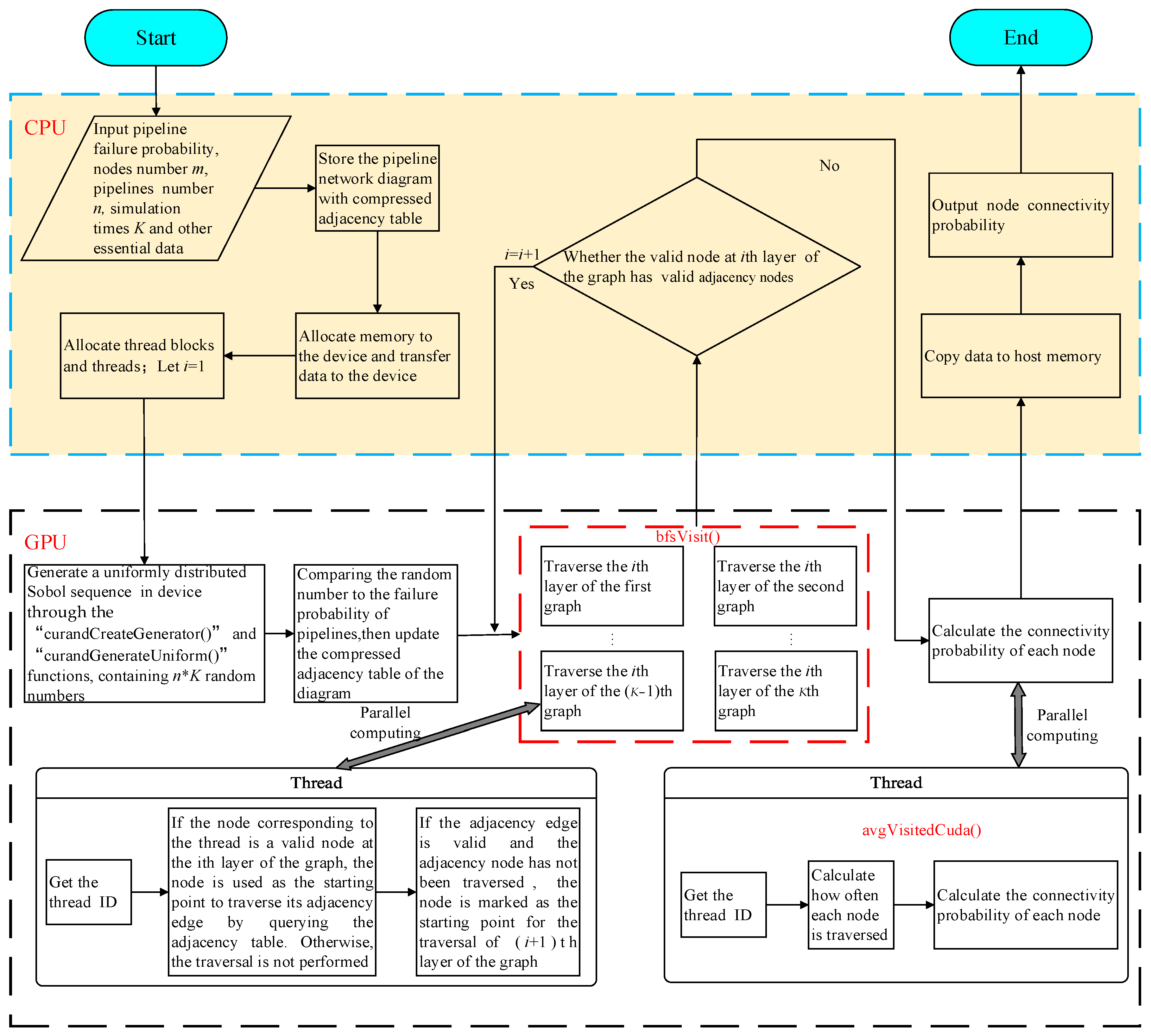
It can be seen from Section 3.3 that the SCR analysis of the WDS requires K QMC simulations. Since each QMC simulation is carried out independently and does not interfere with each other, it has natural parallelism. In addition, in each QMC simulation, when the BFS algorithm is used to calculate the connectivity of the pipe network graph, the adjacent nodes of each layer of vertices can be searched in parallel by multiple threads to shorten the time of traversing the graph. Therefore, this article uses multithreading to process K QMC simulations and BFS traversals of graphs in parallel. The algorithm is based on CUDA using GPU-CPU heterogeneous computing architecture, divided into a CPU processing part and a GPU processing part. The CPU processing part includes the steps of importing basic data of the WDS, generating the adjacency table of the pipe network, transferring data between the host and the device, and allocating the memory of the host and the device. The GPU processing part processes K times for parallel QMC simulations, BFS parallel traversals, and LDS generation to achieve an efficient solution of the SCR analysis of WDS. The logic flow chart of the algorithm of CUDA-based SCR analysis of WDS is shown in Figure 2. The main flow of the algorithm is as follows, for detailed algorithm implementation, see Section 4.2.3.

(1)

Input the basic data such as the total number of nodes m, the total number of pipelines n, the starting point and ending point number of the pipeline, the failure probability of the pipeline under earthquake, the QMC simulation times K in the CPU, and store the pipe network diagram in the format of compressed row storage (CRS) [52].

(2)

Use the “cudaMalloc()” function provided by CUDA to allocate the space in the global graphics memory, and copy the data (i.e., pipe network diagram, number of nodes and pipelines in the pipeline network) from the host memory to the graphics memory through the “cudaMemcpy()” function.

(3)

Generate a uniformly distributed Sobol sequence between 0 and 1 on the GPU through the “curandCreateGenerator()” and “curandGenerateUniform()” functions, containing n*K random numbers. Then, the Sobol sequence is compared with the failure probability of pipelines, and the CRS of K graphs is generated.

(4)

Start the kernel function “bfsVisit()” and implement the BFS traversal of k pipeline network graphs in parallel on the GPU. It should be noted that the kernel function “bfsVisit()” needs to be restarted repeatedly until all the valid nodes are traversed, each time it only searches the valid adjacency nodes of all valid nodes in a certain layer of the pipeline network graph in parallel. Assuming that the adjacency edge of a valid node at the ith layer of the graph is in a reliable state and the corresponding node of the adjacency edge has not been traversed, this node is called a valid adjacency node. The valid adjacency node is defined as the valid node at the (i + 1)th layer of the graph.

(5)

Start the kernel function “avgVisitedCuda()” to calculate the final connection probability of each node in parallel on the GPU.

(6)

Copy the connectivity probability of each node to the CPU and output it.

4.2. CUDA Implementation of the Algorithm

4.2.1. Storage of Graph on the GPU

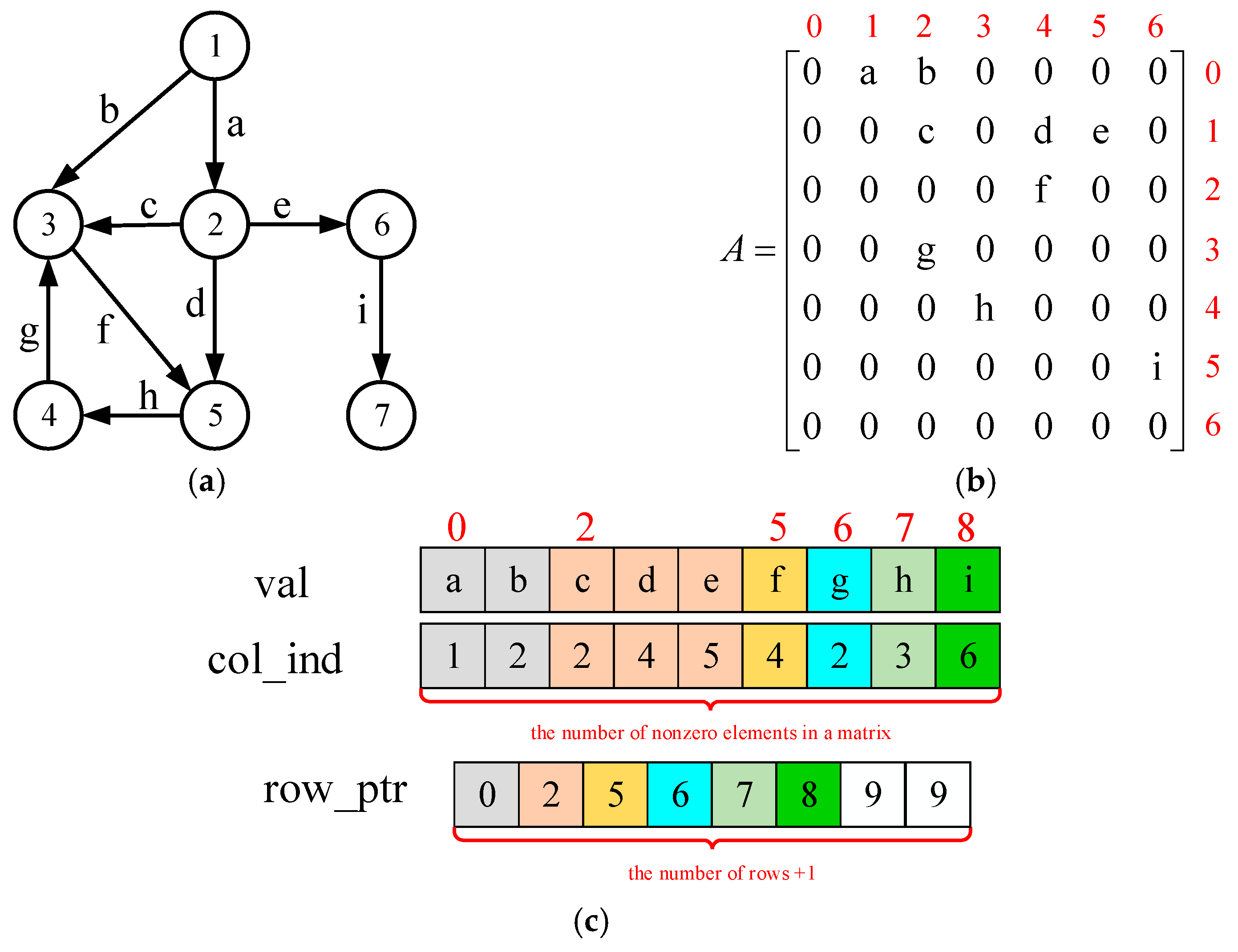
Storing graph data in the GPU requires three considerations: first, the relatively limited capacity of the GPU’s video memory compared to the host’s memory; second, CUDA uses a CPU-GPU heterogeneous computing model in which data are transferred back and forth between the host side and the device side; third, in the CUDA storage system, device memory and host memory have different address spaces, which makes it inconvenient to operate pointer data on the CUDA platform. In addition, since the device memory is abstracted as linear memory, the data structure in the form of an array has the highest access efficiency. Therefore, the CRS format is used to store the pipeline network diagram in the parallel algorithm in the current article. Figure 3c shows the CRS format of the directed edge-weighted graph in Figure 3a. The CRS format uses three arrays to store directed edge-weighted graphs, val array stores the values of nonzero elements in a row-wise fashion, col_ind array stores the corresponding column indices of the elements in the val array, and row_ptr array stores the locations in the val array and col_ind array that start a row.

4.2.2. Sobol Sequence Generation

In the simulation, a large number of quasi-random numbers are used. The cuRAND function library in the CUDA platform provides a pseudo-random number generator and a quasi-random number generator, which can be used to generate random numbers on the host and device. Sobol sequence is the only quasi-random number sequence supported by the host and device API [53]. Therefore, the Sobol sequence is used as the LDS for QMC simulation in this study.

4.2.3. Implementation of the CUDA-Based Reliability Algorithm for WDS

The essence of the parallel algorithm in this study is to use multiple threads to perform multiple BFS traversals on the pipeline network graph at the same time. The pseudocode of the algorithm executed on the host is shown in Algorithm 1. Three arrays, R_a, C_a and V_a are created to store the pipeline network graph G(V, E, W). A float array S_a with the size of eNum * S_n is used to store low-discrepancy random numbers, and an int array P_a and another float array N_a with the size of vNum * S_n are used to store the seismic reliability of each node and the number of layers where the node is located in the pipe network, respectively. First, the number of layers of the source node in each graph is set to 1 through the kernel function “initVisit()” (see Algorithm 2), and then the source nodes are the starting point when traversing pipe network graphs, and the number of layers of other nodes is set to 0. Next, initialise the Boolean variable F to false and the integer variable C_t to 1. In each iteration, it is necessary to determine whether the value of the flag variable F is false, and if so, invoke the kernel function “bfsVisit()” (see Algorithm 3). Then, the flag variable F is set to true, and the nodes whose layer numbers are equal to C_t are treated as the new starting point to traverse the next layer of the pipe network graph. If the connectivity probability of the adjacent edges of the nodes of the current layer is greater than the corresponding low-discrepancy random number, and the number of layers of the adjacent nodes is 0, then the layer of the corresponding adjacent nodes is set to C_t +1, and flag variable F is set to false. It should be noted that the above process is repeated several times until F is true. Finally, the kernel function “avgVisitedCuda()” is activated to calculate the seismic reliability of each node (see Algorithm 4).

Algorithm 1. CUDA BFS (Graph G(V, E, W), Source node S0, Vertex number vNum, Edge number eNum, Simulation number Sn)

1: Create location array Ra, column indices array Ca and weight array Va from G(V, E, W)

2: Create Sobol random numbers array Sa of size eNum * Sn, node traversal array Na of size vNum * Sn, connectivity probability array Pa of size V 3: Invoke CUDA initVisit (Na, vNum, S0) on the grid 4: F ← Flag ← false, Ct ← current_Traversal ← 1 5: while F is false 6:      Invoke CUDA bfsVisit (Ra, Ca, Va, Sa, Ct, Na, F, vNum, eNum) on the grid 7:      Ct ← Ct + 1 8: end while 9: Invoke CUDA avgVisitedCuda (Pa, Na, vNum, Sn) on the grid

Algorithm 2. CUDA initVisit(Na, vNum, S0)

1: tid ← getThreadID 2: v_index ← tid % vNum 3: if v_index + 1 = S0 4:      then Na[tid] ← 1 5:      else Na[tid] ← 0 6: end if

Algorithm 3. CUDA bfsVisit (Ra, Ca, Va, Sa, Ct, Na, F, vNum, eNum)

1: tid ← getThreadID 2: v_index ← id % vNum, sim_index ← tid / vNum, F ← true 3: if Na[tid]= Ct 4:      for i From Ra[v_index] to Ra[v_index + 1] 5:          if Sa[sim_index * eNum + i]< Va[i] 6:              v_index ← Ca[i] 7:              if Na[im_index * vNum + v_index] = 0 8:                  Na[im_index * vNum + v_index] ← Ct + 1 9:                  F ← false 10:              end if 11:          end if 12:     end for 13: end if

Algorithm 4. CUDA avgVisitedCuda (Pa, Na, vNum, Sn)

1: tid ← getThreadID 2: Pa[tid] ← 0 3:    for i From 0 to Sn 4:        if Na[i * vNum + tid] > 0 5:            Pa[tid] ←Pa[tid] + 1 6:        end if 7:    end for 8: Pa[tid] ← Pa[tid] / Sn

5. Numerical Example

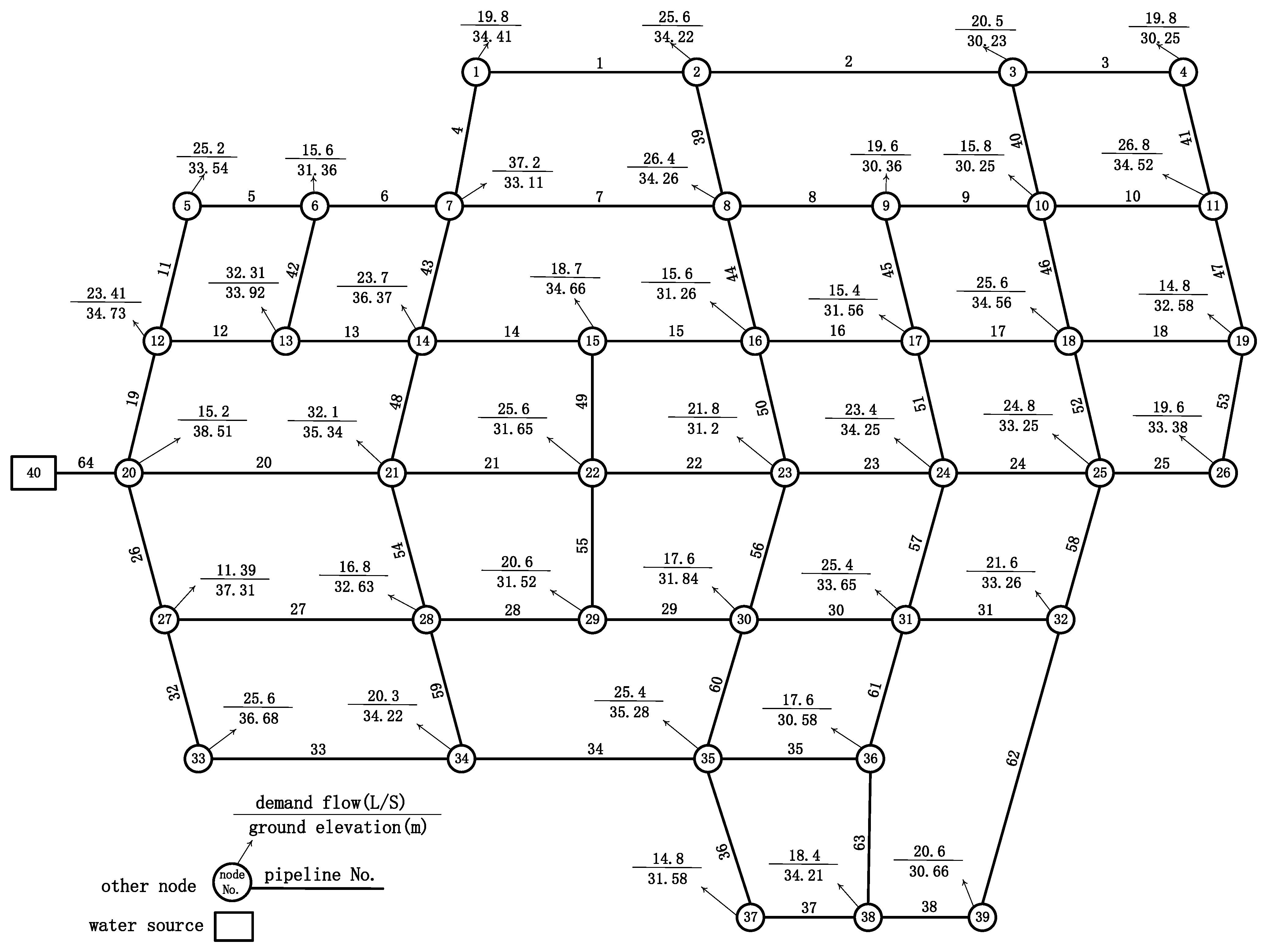
To verify the applicability of the parallel method in this paper, a WDS is taken as an example to analyse its SCR, and the layout of the WDS is shown in Figure 4, which consists of 40 nodes and 64 pipelines. The water supply source is node 40, whose water level is constant at 60 m. The demand flow rate and ground elevation of other nodes can also be seen in Figure 4. Ductile cast iron pipes are adopted in this WDS, and information on pipeline length and diameter is shown in Figure 5. To obtain the probability of different failure states of the pipeline, three kinds of analysis methods are generally adopted, including empirical methods, expert judgment methods and analytic methods. In this study, an empirical method is adopted, and its core idea is to obtain the pipe repair rate (RR) considering pipe type, pipe diameter, site conditions, soil characteristics and other factors by statistical regression of historical earthquake damage data. Furthermore, assuming that the pipeline seismic damage occurs randomly and independently along the pipeline and follows the Poisson distribution, the failure probability P_d of the pipeline can be expressed as follows:

$$P_{\mathrm{d}}=1-e^{-RR\cdot L}$$

(14)

where P_d is the failure probability of the pipeline, including the probability of moderate damage and severe damage; RR is the pipe repair rate, expressed as repairs/km; L is the length (km) of the pipeline.

As shown in Equation (14), the key to using an empirical method to solve pipeline failure probability lies in the determination of the RR. In this study, the RR model proposed by Isoyama et al. is adopted [54], which relates the RR to the peak ground acceleration (PGA) by multiplying some correction factors for the pipeline characteristics, surrounding soil characteristics and topology (see

Table 1. Correction factors.

Category	Subcategory	Correction Factor
Pipe diameter Cd (mm)	Cd < 100	1.6
	100 $\le$ Cd < 200	1.0
	200 $\le$ Cd < 500	0.8
	Cd$\ge$ 500	0.5
Pipe material Cp	ACP	1.2
	VP, PVC	1.0
	CIP	1.0
	PE, HI-3P	0.8
	SP	0.3
	DCIP	0.3
Topography Cg	Narrow valley	3.2
	Terrace	1.5
	Disturbed hill	1.1
	Alluvial	1.0
Liquefaction Cl	Total	2.4
	Partial	2.0
	None	1.0
	Stiff alluvial	0.4

), as shown in the following equations:

RR = C_d × C_p × C_g × C_l × R₀

(15)

R₀ = 2.88 × 10⁻⁶ × (PGA − 100)^1.97

(16)

where C_d, C_p, C_g, and C_l represent the correction factors for the pipe diameter, pipe material, topography, and liquefaction, respectively. R₀ is the standard pipeline RR.

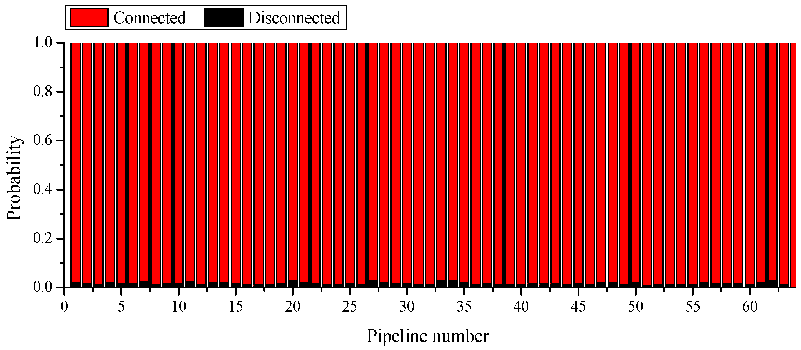
Based on Equations (14)–(16), the failure probabilities of the pipelines under the action of a 9-degree earthquake (0.4 g) are shown in Figure 6. Then the parallel algorithm proposed in Section 4 is used to analyse the SCR of the WDS and compare the results with the traditional serial simulation method based on the Monte Carlo method. It should be noted that both the traditional serial algorithm and the parallel algorithm in this article are implemented in the Visual Studio platform using the C++ programming language. The parallel algorithm is implemented based on the Nvidia CUDA5.0 development kit, and the operating environment is Windows 7. A 2.20-GHz Inter(R)Xeon(R)E5-2407 processor with 4 GB memory and an NVIDIA GeForce GT 610 with 2 GB graphics memory are employed. To verify the accuracy of the parallel method, the serial program and parallel program developed by the author were used to perform 1,000,000 simulations to calculate the seismic connection probability between each node of the pipeline network and the water source under the action of a 9-degree earthquake. As shown in Figure 7, the calculation results of the two methods are basically consistent, and the maximum error is 0.2%, which shows that the parallel method in this paper is correct and meets the accuracy requirements.

To test the computational efficiency of the parallel method in this study, the serial program and the parallel program are used to simulate 3000 times, 5000 times, 10,000 times, 100,000 times, and 1,000,000 times. The simulation times and speedup ratios of the two methods are shown in

Table 2. Comparison of computational time between serial and parallel methods.

Number of Simulations/Times	3000	5000	10,000	100,000	1,000,000
Computation time of serial method/ms	81	103	180	1370	13,454
Computation time of parallel method/ms	45	42	58	262	2222
Speedup ratio	1.80	2.45	3.10	5.23	6.05

and Figure 8, respectively. It can be seen that with the increase in the number of simulations, the program calculation time and speedup ratio of the two methods increase accordingly. When simulating 1,000,000 times, the parallel method can obtain a 6-fold speedup over the serial method, and shorten the calculation time by 11 s, which shows that the parallel method is helpful to improve the efficiency of the SCR analysis of the pipeline network.

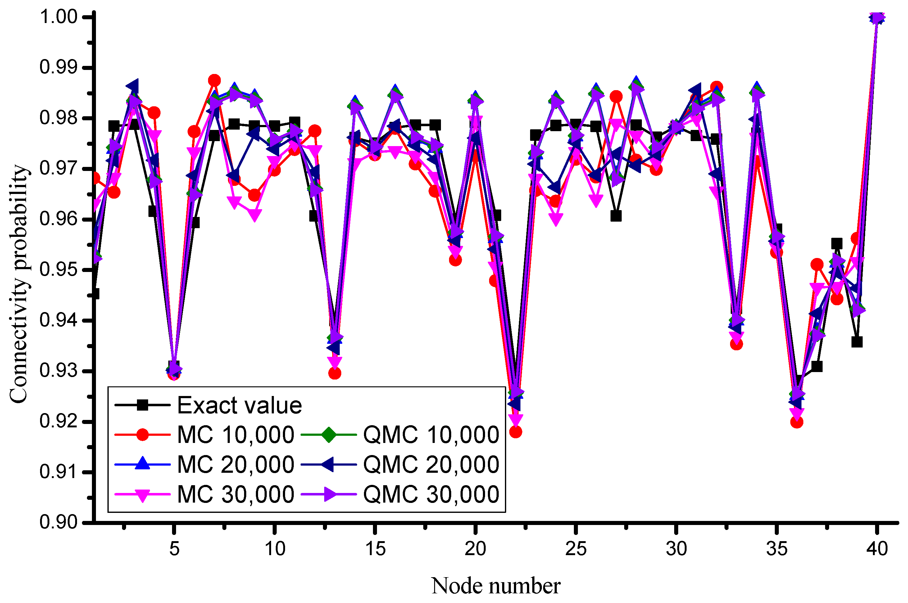
To verify the computational efficiency of the MC and QMC method, the pseudo-random number generator and the Sobol quasi-random number generator are used to generate random number sequences when using parallel method to analyse the SCR of WDS. The MC and QMC methods were used for 10,000, 20,000, and 30,000 simulations, and the SCR analysis result is shown in Figure 9. It needs to be stated that the connection reliability result when the serial program simulates 1,000,000 times is taken as the analytical value, and the influence of the two random number sequences on the error of the calculation result is analysed. As the number of simulations increases, the simulation accuracy of the two methods is improved. When the number of simulations is the same, the simulation result based on the Sobol sequence is more accurate than that based on the pseudo-random number sequence. When simulating 30,000 times, the errors of the parallel method and the parallel method are 0.82% and 1.4%, respectively. When simulating 10,000 times based on the Sobol sequence, the simulation error is 0.95%, which is smaller than the error of simulating 300,000 times based on the pseudo-random number sequence. In general, both methods can meet the simulation accuracy requirements when simulating 10,000 times, while the Sobol sequence can obtain higher precision results with fewer simulations.

To verify the applicability of the parallel method in the SCR analysis of a large-scale pipe network, the pipe network in Figure 4 is spliced, and the scale of the pipe networks after splicing is shown in

Table 3. Comparison of the time consumption of the two methods to calculate the SCR of different scale pipe networks.

Number of Stitches	Number of Nodes	Number of Pipelines	Computation Time of Parallel Method/ms	Computation Time of Serial Method/ms
1	40	64	58	180
5	201	325	250	590
10	401	650	500	1089
15	601	975	745	1568
20	801	1300	1032	2567
25	1001	1625	1165	4524

. Serial and parallel programs are used to analyse the SCR of the spliced pipe network. The simulation time of the two methods when simulating 10,000 times are shown in Table 3. It can be seen from Table 3 that when analysing different scale pipe networks, the parallel algorithm can achieve effective acceleration compared with the serial method. When the number of nodes is 1001, a 4-fold speedup ratio can be obtained.

6. Conclusions

With the continuous expansion of the WDS scale, it is of great significance to accurately and quickly predict and evaluate the SCR of pipe networks under earthquake action. In this paper, we leverage the immense computational power of GPU to devise an efficient algorithm for SCR analysis of WDS, enabling rapid assessment of a WDS’s functional capacity at first glance.

Based on graph theory, the WDS is abstracted into a directed edge-weight graph, and combined with the BFS algorithm, the QMC method of replacing the traditional pseudo-random number sequence with the Sobol sequence is applied to the SCR analysis of the WDS. Through example analysis, it is shown that the QMC method has higher computational efficiency and accuracy than the traditional MC method.

The parallelism of the SCR analysis of the WDS is analysed, and a parallel algorithm for SCR analysis based on the QMC method is proposed and programmed by combining the CUDA platform. Example analysis shows that the results calculated by the parallel algorithm proposed in this paper and the traditional serial method are almost consistent, which shows that the parallel method proposed is correct and meets the accuracy requirements and verifies the rationality of the parallel algorithm. When the scale of the pipe network remains unchanged, with the increase in the number of simulations, the acceleration effect of the parallel algorithm is more obvious than that of the serial method. When the number of simulations remains unchanged, the parallel algorithm has more advantages as the scale of the pipe network increases.

The parallel method proposed in this article is versatile and can also be applied to the seismic reliability analysis of other lifeline systems (gas supply system, road and bridge system, power system, etc.).

References

1. Büyüksaraç, A.; Işık, E.; Bektaş, Ö. A comparative evaluation of earthquake code change on seismic parameter and structural analysis; a case of Turkey. Arab. J. Sci. Eng. 2022, 47, 12301–12321. [Google Scholar] [CrossRef]
2. Dal Zilio, L.; Ampuero, J.P. Earthquake doublet in Turkey and Syria. Commun. Earth Environ. 2023, 4, 71. [Google Scholar] [CrossRef]
3. Cui, P.; Chen, X.-Q.; Zhu, Y.-Y.; Su, F.-H.; Wei, F.-Q.; Han, Y.-S.; Liu, H.-J.; Zhuang, J.-Q. The Wenchuan Earthquake (May 12, 2008), Sichuan Province, China, and resulting geohazards. Nat. Hazards 2011, 56, 19–36. [Google Scholar] [CrossRef]
4. Bata, M.T.H.; Carriveau, R.; Ting, D.S.-K. Urban water supply systems’ resilience under earthquake scenario. Sci. Rep. 2022, 12, 20555. [Google Scholar] [CrossRef] [PubMed]
5. Hasan, M.A. Performance of Water Supply Lines in a Post-Earthquake Scenario. Pol. J. Environ. Stud. 2021, 30, 4545–4554. [Google Scholar] [CrossRef]
6. Bouziou, D.; O’rourke, T. Response of the Christchurch water distribution system to the 22 February 2011 earthquake. Soil Dyn. Earthq. Eng. 2017, 97, 14–24. [Google Scholar] [CrossRef]
7. Eidinger, J.M. Performance of Water Systems during the Manic M-w 8.8 Earthquake of 27 February 2010. Earthq. Spectra 2012, 28, 605–620. [Google Scholar] [CrossRef]
8. Zhou, Y.; Chen, L.; Long, L. Modeling cyclic behavior of squat reinforced concrete walls exposed to acid deposition. J. Build. Eng. 2023, 63, 105432. [Google Scholar] [CrossRef]
9. Zhou, Y.; Zheng, S.; Chen, L.; Long, L.; Wang, B. Experimental investigation into the seismic behavior of squat reinforced concrete walls subjected to acid rain erosion. J. Build. Eng. 2021, 44, 102899. [Google Scholar] [CrossRef]
10. Long, L.; Zheng, S.S.; Zhou, Y.; He, J.C.; Meng, H.L.; Cai, Y.L. Parallel study of seismic reliability analysis of water supply pipe network based on quasi-Monte Carlo method. J. Zhejiang Univ. Eng. Sci. 2020, 54, 241–247. [Google Scholar]
11. Liu, X.H.; He, J.C.; Zheng, S.S.; Chen, D.X.; Wu, X.X. Lifeline: Modeling the Impact of Power Systems on Seismic Reliability of Water Supply Systems. J. Tianjin Univ. 2021, 54, 468–478. [Google Scholar]
12. Kim, Y.; Kang, W.H. Network reliability analysis of complex systems using a non-simulation-based method. Reliab. Eng. Syst. Saf. 2013, 110, 80–88. [Google Scholar] [CrossRef]
13. Wagner, J.M.; Shamir, U.; Marks, D.H. Water distribution reliability: Analytical methods. J. Water Resour. Plan. Manag. 1988, 114, 253–275. [Google Scholar] [CrossRef]
14. Kuo, S.-Y.; Lu, S.-K.; Yeh, F.-M. Determining terminal-pair reliability based on edge expansion diagrams using OBDD. IEEE Trans. Reliab. 1999, 48, 234–246. [Google Scholar] [CrossRef]
15. Aggarwal, K.K.; Misra, K.B.; Gupta, J.S. A fast algorithm for reliability evaluation. IEEE Trans. Reliab. 1975, 24, 83–85. [Google Scholar] [CrossRef]
16. Lin, H.-Y.; Kuo, S.-Y.; Yeh, F.-M. Minimal cutset enumeration and network reliability evaluation by recursive merge and BDD. In Proceedings of the Eighth IEEE Symposium on Computers and Communications, Kemer-Antalya, Turkey, 30 June–3 July 2003; pp. 1341–1346. [Google Scholar]
17. Yoo, Y.; Deo, N. A comparison of algorithms for terminal-pair reliability. IEEE Trans. Reliab. 1988, 37, 210–215. [Google Scholar] [CrossRef]
18. Torrieri, D. Calculation of node-pair reliability in large networks with unreliable nodes. IEEE Trans. Reliab. 1994, 43, 375–377. [Google Scholar] [CrossRef]
19. Selcuk, A.S.; Yücemen, M.S. Reliability of lifeline networks under seismic hazard. Reliab. Eng. Syst. Saf. 1999, 65, 213–227. [Google Scholar] [CrossRef]
20. Li, J.; He, J. A recursive decomposition algorithm for network seismic reliability evaluation. Earthq. Eng. Struct. Dyn. 2002, 31, 1525–1539. [Google Scholar] [CrossRef]
21. Shinozuka, M.; Tan, R.; Toike, T. Serviceability of water transmission systems under seismic risk. In Lifeline Earthquake Engineering: The Current State of Knowledge; American Society of Civil Engineers: New York, NY, USA, 1981. [Google Scholar]
22. Adachi, T.; Ellingwood, B.R. Serviceability of earthquake-damaged water systems: Effects of electrical power availability and power backup systems on system vulnerability. Reliab. Eng. Syst. Saf. 2008, 93, 78–88. [Google Scholar] [CrossRef]
23. Fishman, G.S. A Comparison of Four Monte Carlo Methods for Estimating the Probability of s-t Connectedness. IEEE Trans. Reliab. 1986, 35, 145–155. [Google Scholar] [CrossRef]
24. Metropolis, N.; Ulam, S. The monte carlo method. J. Am. Stat. Assoc. 1949, 44, 335–341. [Google Scholar] [CrossRef] [PubMed]
25. James, F. Monte Carlo theory and practice. Rep. Prog. Phys. 1980, 43, 1145. [Google Scholar] [CrossRef]
26. Soboĺ, I.M. Quasi-monte carlo methods. Prog. Nucl. Energy 1990, 24, 55–61. [Google Scholar] [CrossRef]
27. Selcuk-Kestel, A.S.; Duzgun, H.S.; Oduncuoglu, L. A GIS-based software for lifeline reliability analysis under seismic hazard. Comput. Geosci. 2012, 42, 37–46. [Google Scholar] [CrossRef]
28. Ciaponi, C.; Franchioli, L.; Papiri, S. Simplified Procedure for Water Distribution Networks Reliability Assessment. J. Water Resour. Plan. Manag. 2012, 138, 368–376. [Google Scholar] [CrossRef]
29. Oliveira, G.C.; Pereira, M.V.; Cunha, M.V. A technique for reducing computational effort in Monte-Carlo based composite re-liability evaluation. IEEE Trans. Power Syst. 1989, 4, 1309–1315. [Google Scholar] [CrossRef]
30. Keramat, M.; Kielbasa, R. A study of stratified sampling in variance reduction techniques for parametric yield estimation. IEEE Trans. Circuits Syst. II Analog. Digit. Signal Process. 1998, 45, 575–583. [Google Scholar] [CrossRef]
31. Ferrenberg, A.M.; Swendsen, R.H. Optimized monte carlo data analysis. Comput. Phys. 1989, 3, 101–104. [Google Scholar] [CrossRef]
32. Boyle, P.; Broadie, M.; Glasserman, P. Monte Carlo methods for security pricing. J. Econ. Dyn. Control. 1997, 21, 1267–1321. [Google Scholar] [CrossRef]
33. Dai, H.Z.; Wang, W. Application of low-discrepancy sampling method in structural reliability analysis. Struct. Saf. 2009, 31, 55–64. [Google Scholar] [CrossRef]
34. Singhee, A.; Rutenbar, R.A. Why Quasi-Monte Carlo is Better Than Monte Carlo or Latin Hypercube Sampling for Statistical Circuit Analysis. IEEE Trans. Comput. Des. Integr. Circuits Syst. 2010, 29, 1763–1776. [Google Scholar] [CrossRef]
35. Luebke, D.; Harris, M. General-purpose computation on graphics hardware. In Proceedings of the Workshop: SIGGRAPH, Singapore, 16–18 June 2004; Volume 33, p. 6. [Google Scholar]
36. Garland, M.; Le Grand, S.; Nickolls, J.; Anderson, J.; Hardwick, J.; Morton, S.; Phillips, E.; Zhang, Y.; Volkov, V. Parallel Computing Experiences with CUDA. IEEE Micro 2008, 28, 13–27. [Google Scholar] [CrossRef]
37. Spiechowicz, J.; Kostur, M.; Machura, L. GPU accelerated Monte Carlo simulation of Brownian motors dynamics with CUDA. Comput. Phys. Commun. 2015, 191, 140–149. [Google Scholar] [CrossRef]
38. Nielsen, C. GPU accelerated Monte Carlo simulation of high-intensity pulsed laser-electron interaction. Comput. Phys. Commun. 2022, 278, 108425. [Google Scholar] [CrossRef]
39. Brost, E.E.; Tseung, H.W.C.; Antolak, J.A. A fast GPU-accelerated Monte Carlo engine for calculation of MLC-collimated electron fields. Med. Phys. 2022, 50, 600–618. [Google Scholar] [CrossRef]
40. Feng, H.; Patel, S.H.; Wong, W.W.; Younkin, J.E.; Penoncello, G.P.; Morales, D.H.; Stoker, J.B.; Robertson, D.G.; Fatyga, M.; Bues, M.; et al. GPU-accelerated Monte Carlo-based online adaptive proton therapy: A feasibility study. Med. Phys. 2022, 49, 3550–3563. [Google Scholar] [CrossRef]
41. West, D.B. Introduction to Graph Theory; Prentice Hall: Upper Saddle River, NJ, USA, 2001. [Google Scholar]
42. Harary, F. The Determinant of the Adjacency Matrix of a Graph. SIAM Rev. 1962, 4, 202–210. [Google Scholar] [CrossRef]
43. Fulkerson, D.; Gross, O. Incidence matrices and interval graphs. Pac. J. Math. 1965, 15, 835–855. [Google Scholar] [CrossRef]
44. Singh, H.; Sharma, R. Role of adjacency matrix & adjacency list in graph theory. Int. J. Comput. Technol. 2012, 3, 179–183. [Google Scholar]
45. Deng, Q.L.; Jiang, Z.A.; Han, S.; Fu, E.Q. Reliability Analysis of Dust-Proof Water Supply Network System Based on Sobol. J. Tianjin Univ. Sci. Technol. 2018, 51, 919–926. [Google Scholar]
46. Niederreiter, H. Random Number Generation and Quasi-Monte Carlo Methods; Society for Industrial and Applied Mathematics: Siam, PA, USA, 1992. [Google Scholar]
47. Halton, J.H. On the efficiency of certain quasi-random sequences of points in evaluating multi-dimensional integrals. Numer. Math. 1960, 2, 84–90. [Google Scholar] [CrossRef]
48. Sobol, I.M. On the distribution of points in a cube and the approximate evaluation of integrals. Zhurnal Vychislitel’noi Matemat. I Mat. Fiz. 1967, 7, 784–802. [Google Scholar] [CrossRef]
49. McKay, M.D.; Beckman, R.J.; Conover, W.J. A comparison of three methods for selecting values of input variables in the analy-sis of output from a computer code. Technometrics 2000, 42, 55–61. [Google Scholar] [CrossRef]
50. Antonov, I.A.; Saleev, V.M. An economic method of computing LPτ-sequences. USSR Comput. Math. Math. Phys. 1979, 19, 252–256. [Google Scholar] [CrossRef]
51. Bundy, A.; Wallen, L. Breadth-first search. In Catalogue of Artificial Intelligence Tools; Springer: Berlin, Germany, 1984. [Google Scholar]
52. Harish, P.; Narayanan, P.J. Accelerating large graph algorithms on the GPU using CUDA. In High Performance Computing–HiPC 2007, Proceedings of the 14th International Conference, Goa, India, 18–21 December 2007; Springer: Berlin/Heidelberg, Germany, 2007; pp. 197–208. [Google Scholar]
53. Cheng, J.; Grossman, M.; McKercher, T. Professional CUDA C Programming; John Wiley & Sons: Hoboken, NJ, USA, 2014. [Google Scholar]
54. Isoyama, R.; Ishida, E.; Yune, K.; Shirozu, T. Seismic damage estimation procedure for water supply pipelines. Water Supply 2000, 18, 63–68. [Google Scholar]
Figure 1. Two-dimensional distribution of pseudo-random sequence and Sobol sequence. (a) Pseudo-random sequence. (b) Sobol sequence.
Water 15 02087 g001
Figure 2. Logical flow chart of the parallel algorithm for SRC analysis of WDS based on CUDA.
Water 15 02087 g002
Figure 3. Storage form of directed edge-weighted graph. (a) Directed edge-weighted graph. (b) Adjacent matrix. (c) Compressed row storage.
Water 15 02087 g003
Figure 4. Layout diagram of the WDS.
Water 15 02087 g004
Figure 5. Basic information of the WDS.
Water 15 02087 g005
Figure 6. Failure probabilities of pipelines under the action of a 9-degree earthquake.
Water 15 02087 g006
Figure 7. Connectivity probability of each node based on serial and parallel methods.
Water 15 02087 g007
Figure 8. Speedup ratio of the parallel method when different times are simulated.
Water 15 02087 g008
Figure 9. Comparison of the simulation results of the MC and QMC methods.
Water 15 02087 g009