
Machine Learning Algorithms for the Estimation of Water Quality Parameters in Lake Llanquihue in Southern Chile

 ,
, 
 ,
,  ,
,  ,
,
Abstract
1. Introduction
2. Materials and Methods
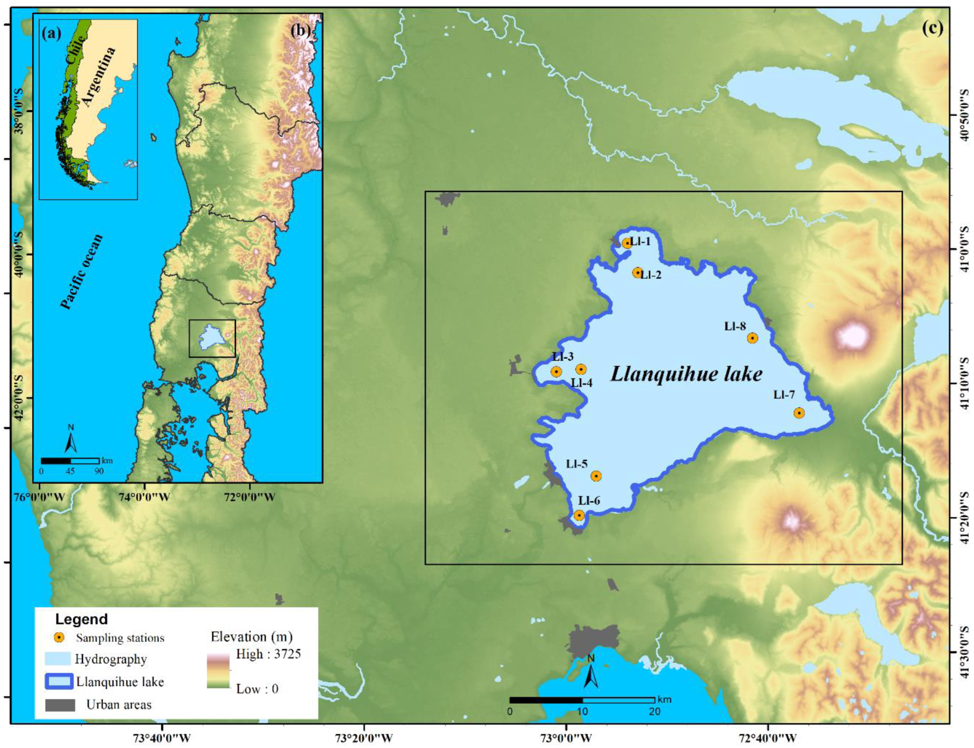
2.1. Study Area
2.2. In Situ Monitoring Data
2.3. Data Wrangling and Features Engineering
- Remove non-numerical values from each of the selected variables and replace them with null values.
- Extract the year, month, and day for each measurement, verifying consistency and integrity.
- Apply sensible imputation for the null values of each column using a robust central tendency measurement, the median.
- Split data for training and test validation. In total, for all measurements, the first 80% collected at each sampling station over time were selected for training, and the remaining 20% were used for testing (Table 1).
- Standardize numerical variables (N, P, Si, DQO, O_D, O_D_sat, PH, Temp, Wind, Hum, Conduct, Trans, and Chl) using the PowerTransformer method, a technique for transforming numerical input or output variables to have a uniform or a Gaussian probability distribution. A power transform will make the probability distribution of a variable more Gaussian [48].
2.4. Machine and Deep Learning Algorithms
| Random Forest Algorithm |
|
| AdaBoost Algorithm |
|
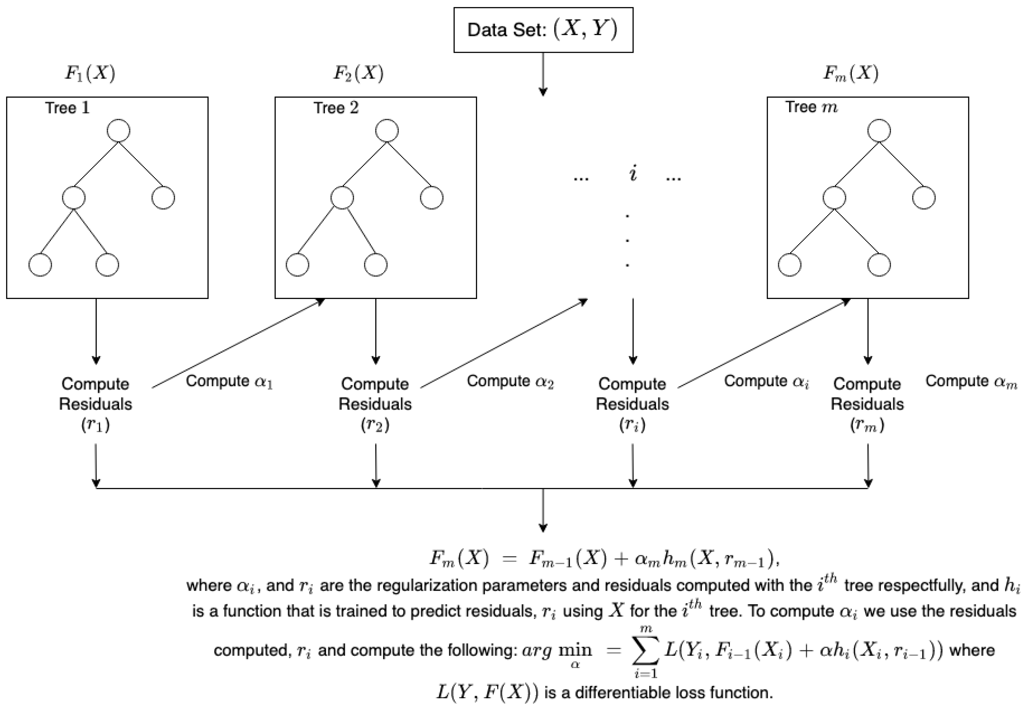
| Gradient Boosting Algorithm |
|
| LightGBM Algorithm |
|
2.5. K-Fold Cross-Validation
2.6. Hyperparameter Tuning
2.7. Performance Metrics
2.7.1. Mean Absolute Error
2.7.2. Root-Mean-Square Error
2.7.3. Coefficient of Determination
2.8. Collection and Treatment of Samples for the Identification of Algal Groups
3. Results
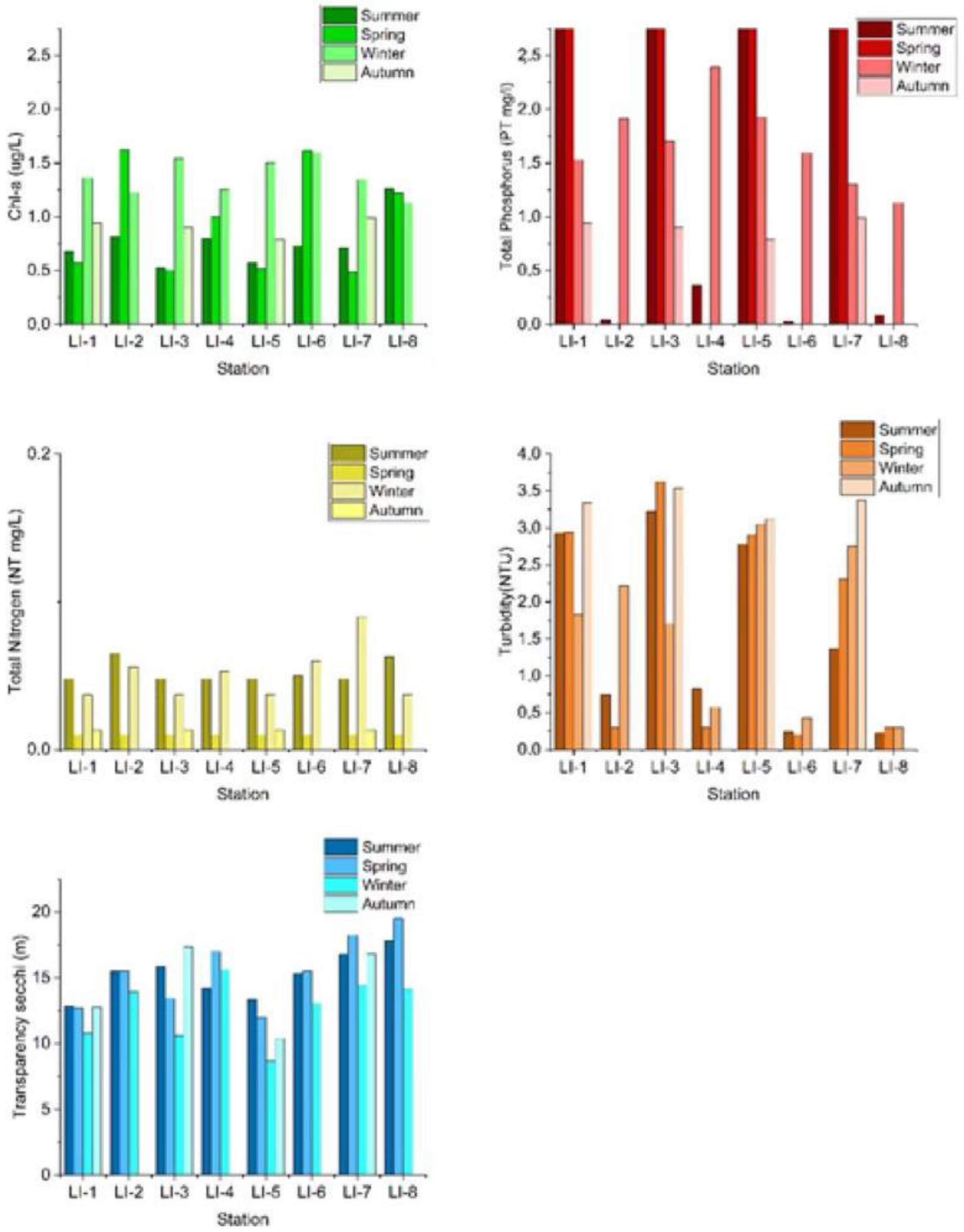
3.1. Water Quality Parameters Summary
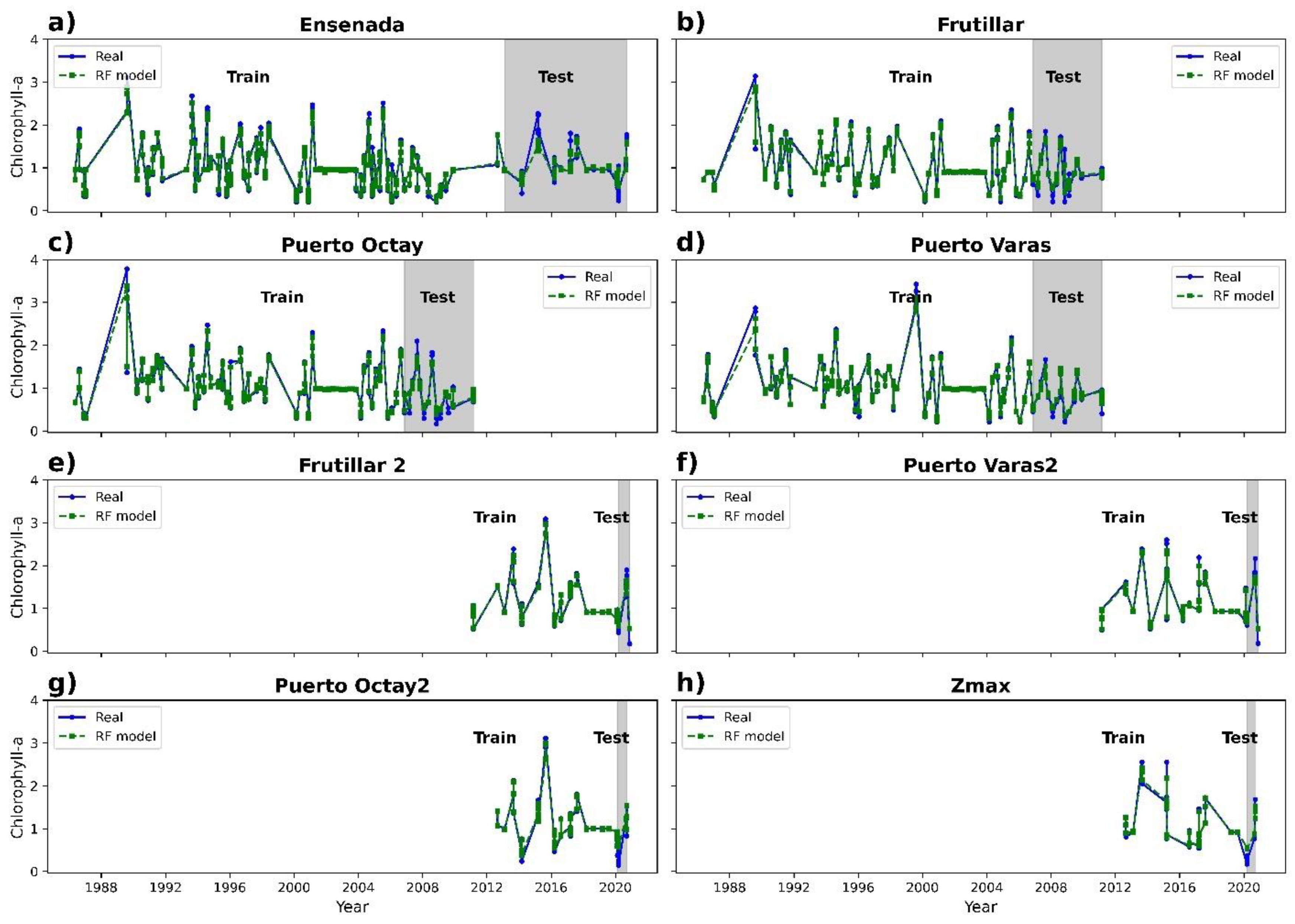
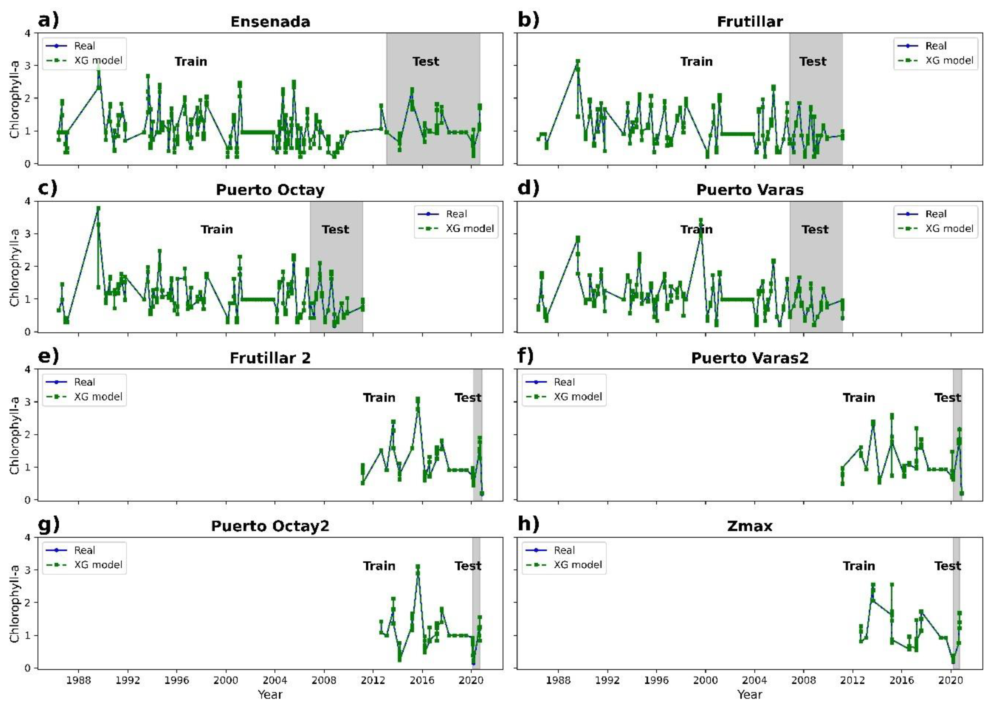
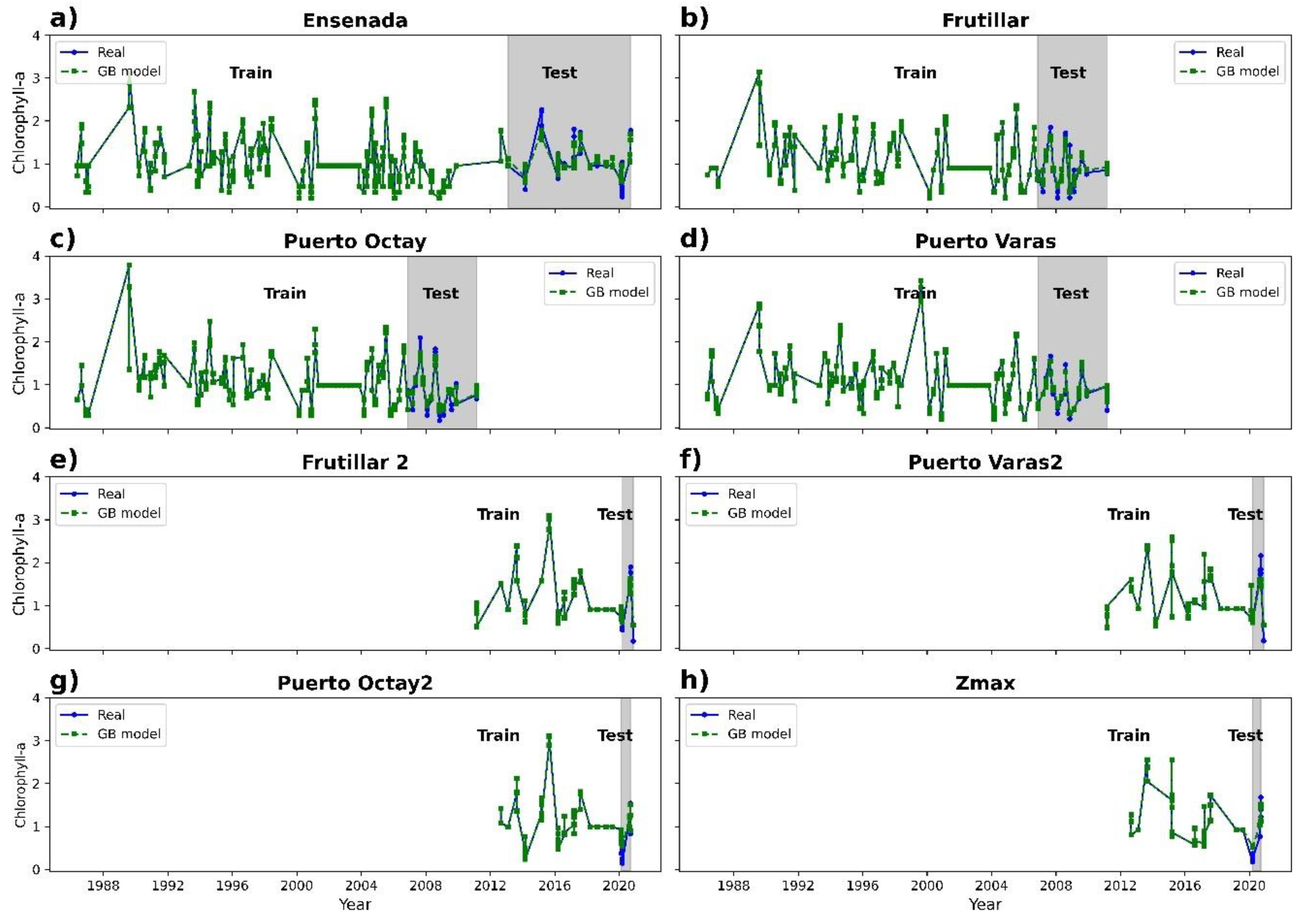
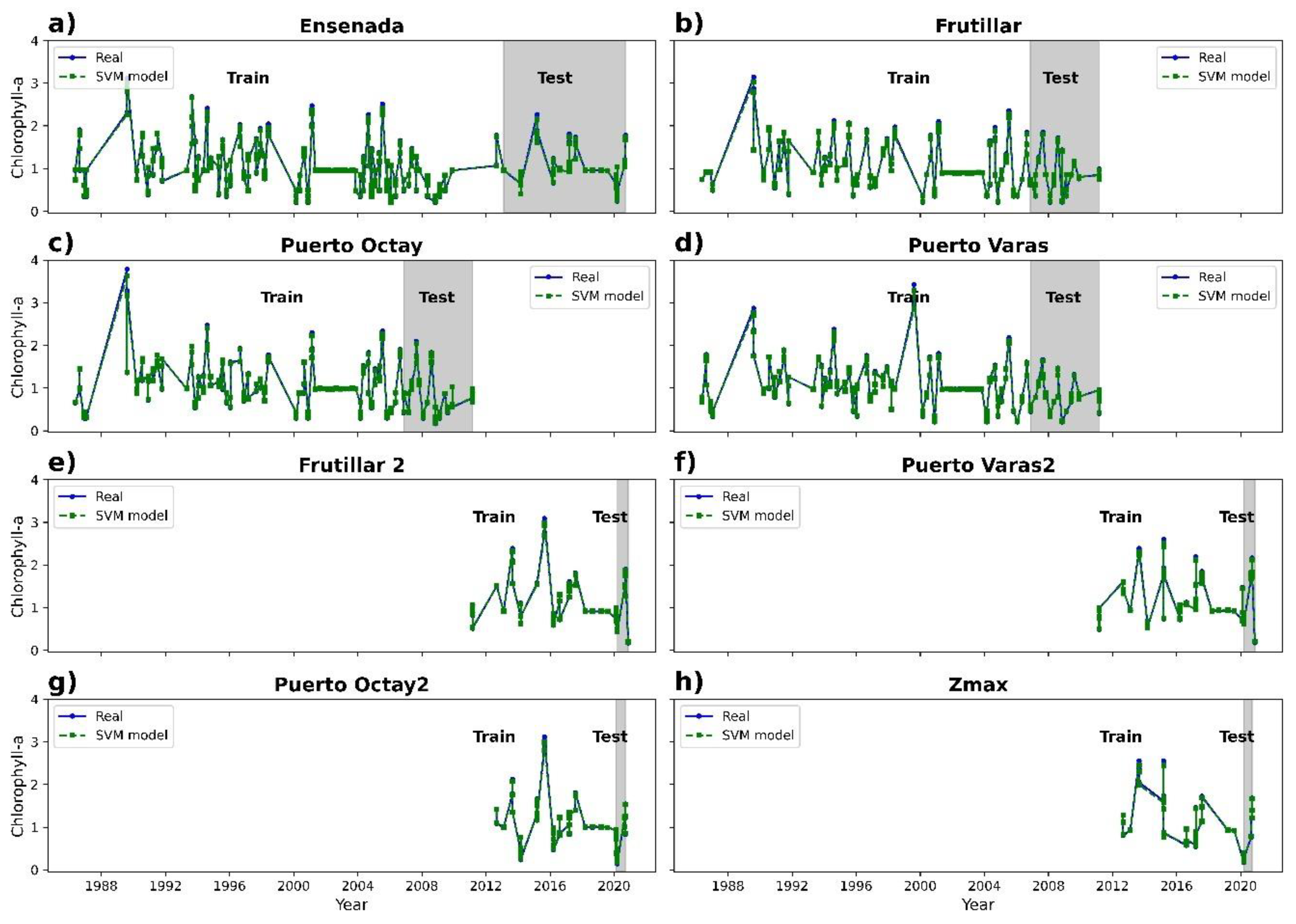
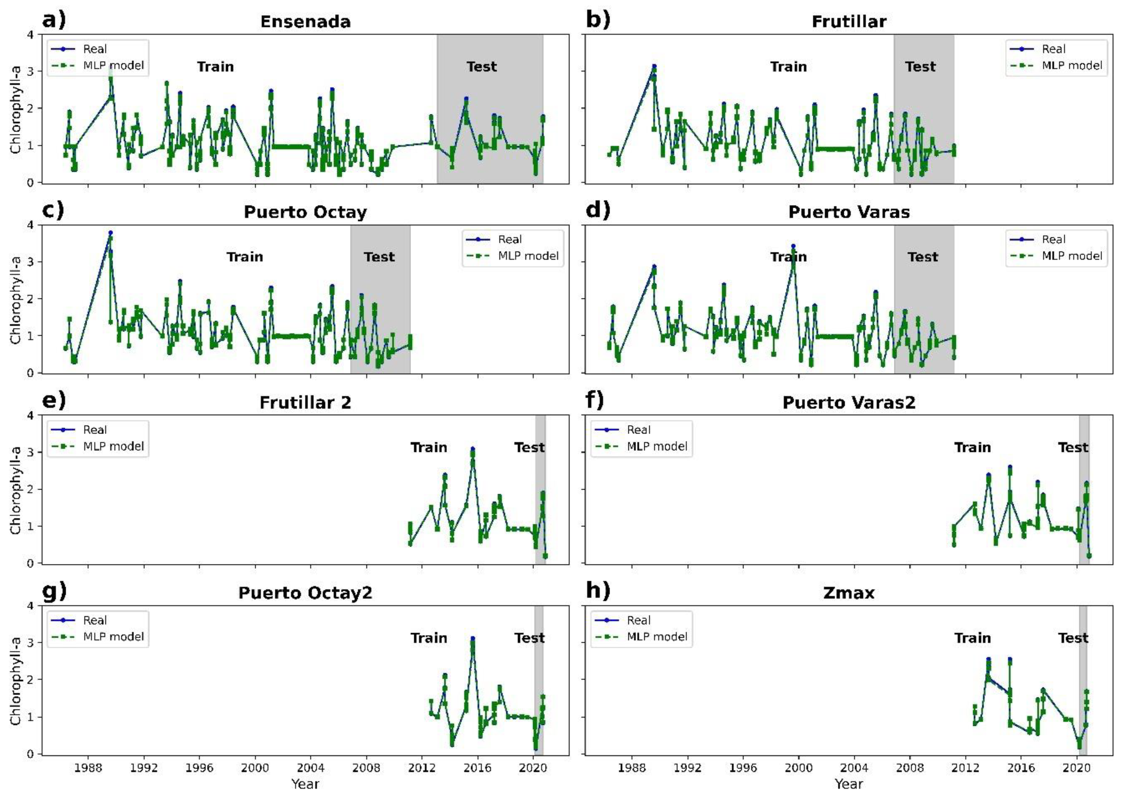
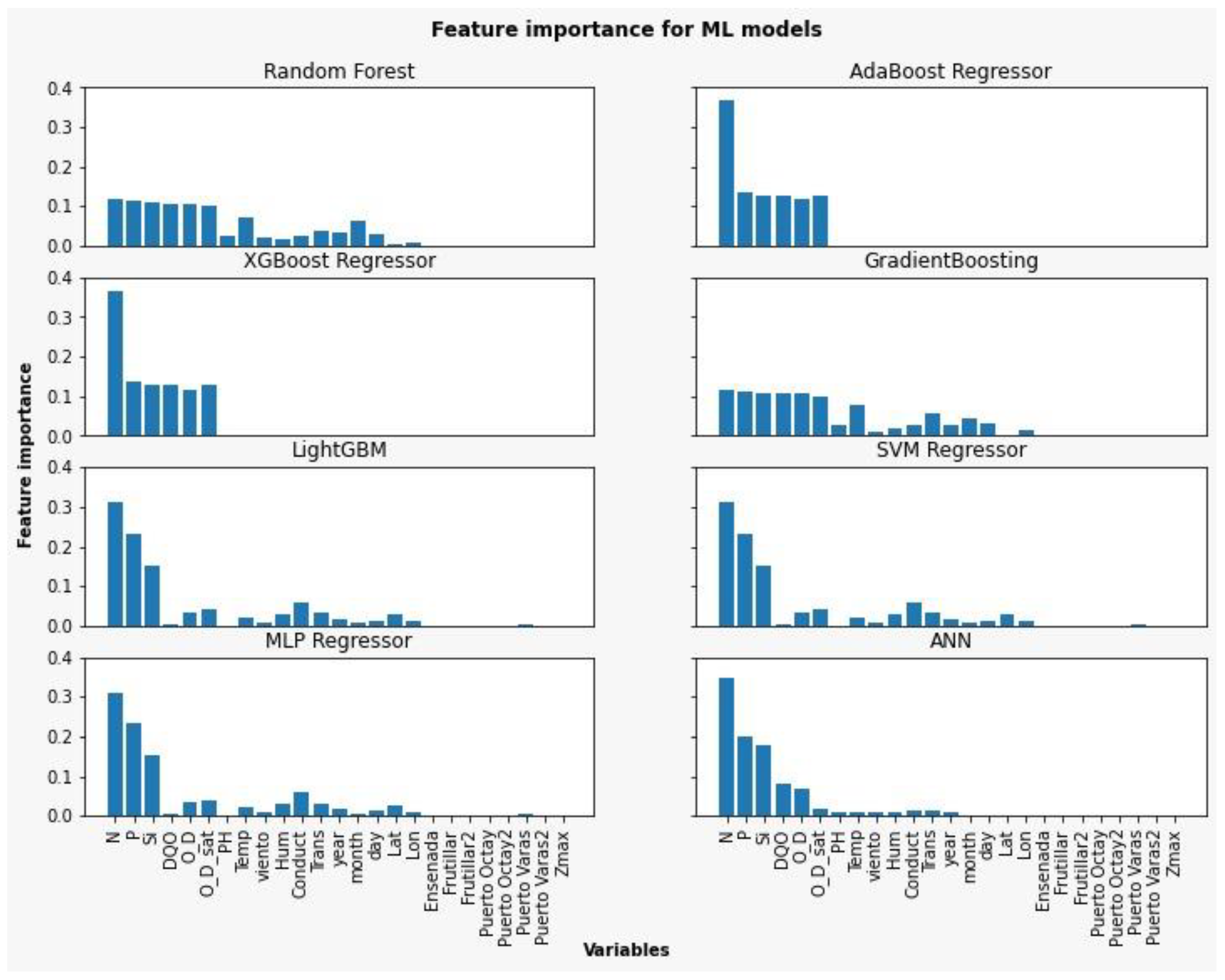
3.2. Chlorophyll-a Prediction
3.3. Statistical Analysis
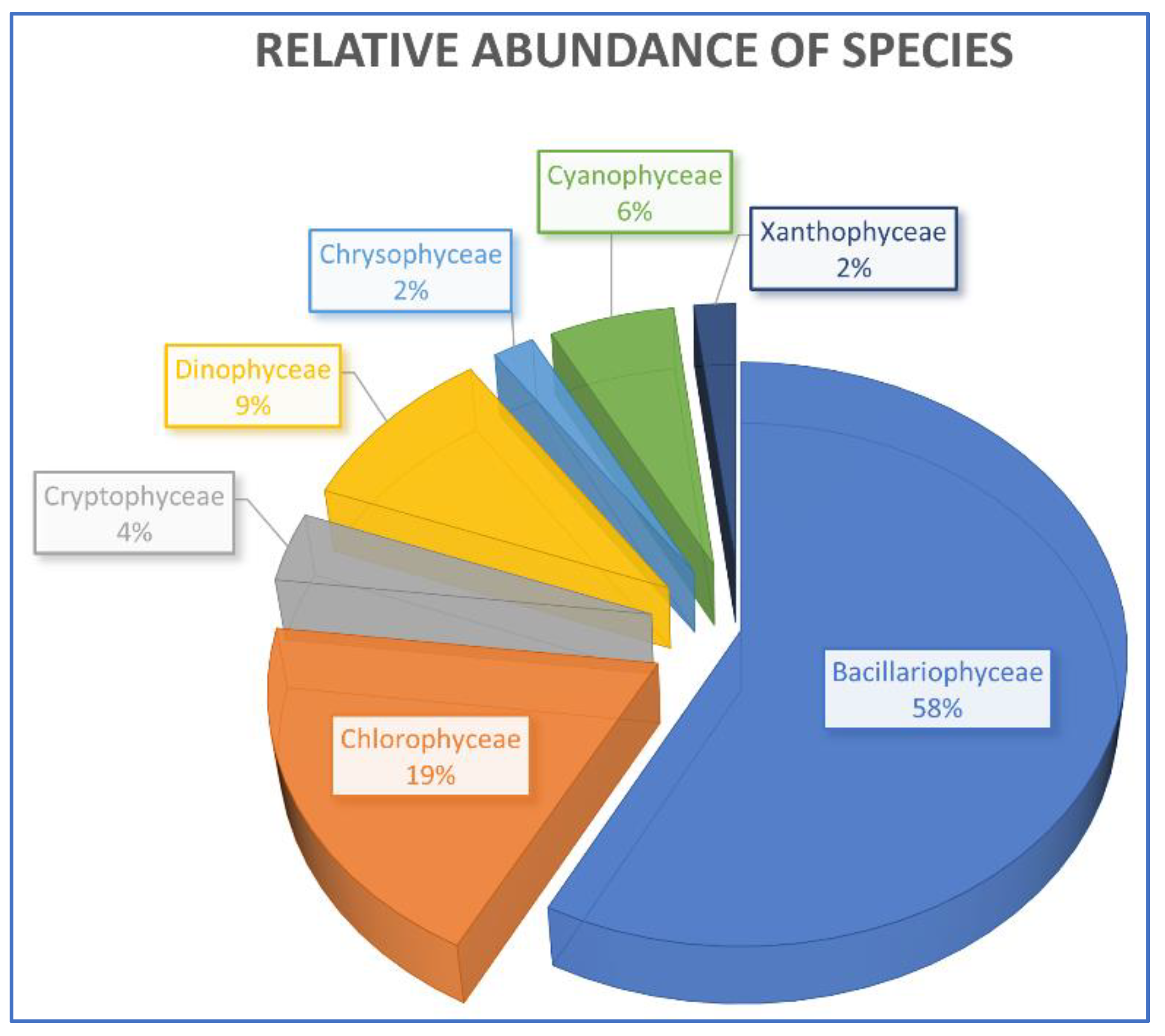
3.4. Specific Composition and Relative Abundance
4. Discussion
5. Conclusions
Supplementary Materials
Author Contributions
Funding
Institutional Review Board Statement
Informed Consent Statement
Data Availability Statement
Acknowledgments
Conflicts of Interest
References
- Prakash, S. Impact of climate change on aquatic ecosystem and its biodiversity: An overview. Int. J. Biol. Innov. 2021, 3, 312–317. [Google Scholar] [CrossRef]
- Yin, S.; Yi, Y.; Liu, Q.; Luo, Q.; Chen, K. A Review on Effects of Human Activities on Aquatic Organisms in the Yangtze River Basin since the 1950s. River 2022, 1, 104–119. [Google Scholar] [CrossRef]
- Wetzel, R. Limnology: Lake and River Ecosystems; Gulf Professional Publishing: Oxford, UK, 2001. [Google Scholar]
- Okello, C.; Tomasello, B.; Greggio, N.; Wambiji, N.; Antonellini, M. Impact of Population Growth and Climate Change on the Freshwater Resources of Lamu Island, Kenya. Water 2015, 7, 1264–1290. [Google Scholar] [CrossRef]
- Boretti, A.; Rosa, L. Reassessing the Projections of the World Water Development Report. NPJ Clean Water 2019, 2, 15. [Google Scholar] [CrossRef]
- Arthington, A.H.; Dulvy, N.K.; Gladstone, W.; Winfield, I.J. Fish Conservation in Freshwater and Marine Realms: Status, Threats and Management. Aquat. Conserv. Mar. Freshw. Ecosyst. 2016, 26, 838–857. [Google Scholar] [CrossRef]
- Decaëns, T.; Martins, M.B.; Feijoo, A.; Oszwald, J.; Dolédec, S.; Mathieu, J.; Arnaud de Sartre, X.; Bonilla, D.; Brown, G.G.; Cuellar Criollo, Y.A.; et al. Biodiversity Loss along a Gradient of Deforestation in Amazonian Agricultural Landscapes. Conserv. Biol. 2018, 32, 1380–1391. [Google Scholar] [CrossRef] [PubMed]
- Valdés-Pineda, R.; García-Chevesich, P.; Valdés, J.B.; Pizarro-Tapia, R. The First Drying Lake in Chile: Causes and Recovery Options. Water 2020, 12, 290. [Google Scholar] [CrossRef]
- Ocampo-Melgar, A.; Barria, P.; Chadwick, C.; Diaz-Vasconcellos, R. Rural Transformation and Differential Vulnerability: Exploring Adaptation Strategies to Water Scarcity in the Aculeo Lake Basin (Chile). Front. Environ. Sci. 2022, 10, 955023. [Google Scholar] [CrossRef]
- Palmeirim, A.F.; Santos-Filho, M.; Peres, C.A. Marked Decline in Forest-Dependent Small Mammals Following Habitat Loss and Fragmentation in an Amazonian Deforestation Frontier. PLoS ONE 2020, 15, e0230209. [Google Scholar] [CrossRef]
- Rodríguez-López, L.; Duran-Llacer, I.; González-Rodríguez, L.; Abarca-del-Rio, R.; Cárdenas, R.; Parra, O.; Martínez-Retureta, R.; Urrutia, R. Spectral Analysis Using LANDSAT Images to Monitor the Chlorophyll-a Concentration in Lake Laja in Chile. Ecol. Inf. 2020, 60, 101183. [Google Scholar] [CrossRef]
- Giralt, D.; Pantoja, J.; Morales, M.B.; Traba, J.; Bota, G. Landscape-Scale Effects of Irrigation on a Dry Cereal Farmland Bird Community. Front. Ecol. Evol. 2021, 9, 611563. [Google Scholar] [CrossRef]
- Sun, Y.; Mao, X.; Gao, T.; Liu, H.; Zhao, Y. Potential Water Withdrawal Reduction to Mitigate Riverine Ecosystem Degradation under Hydropower Development: A Computable General Equilibrium Model Analysis. River Res. Appl. 2021, 37, 1223–1230. [Google Scholar] [CrossRef]
- Newsome, D. The Collapse of Tourism and Its Impact on Wildlife Tourism Destinations. J. Tour. Futur. 2020, 7, 295–302. [Google Scholar] [CrossRef]
- Rodríguez-López, L.; González-Rodríguez, L.; Duran-Llacer, I.; García, W.; Cardenas, R.; Urrutia, R. Assessment of the Diffuse Attenuation Coefficient of Photosynthetically Active Radiation in a Chilean Lake. Remote Sens. 2022, 14, 4568. [Google Scholar] [CrossRef]
- Bai, Y.; Ochuodho, T.O.; Yang, J. Impact of Land Use and Climate Change on Water-Related Ecosystem Services in Kentucky, USA. Ecol. Indic. 2019, 102, 51–64. [Google Scholar] [CrossRef]
- Rodríguez-López, L.; González-Rodríguez, L.; Duran-Llacer, I.; Cardenas, R.; Urrutia, R. Spatio-Temporal Analysis of Chlorophyll in Six Araucanian Lakes of Central-South Chile from Landsat Imagery. Ecol. Inf. 2021, 65, 101431. [Google Scholar] [CrossRef]
- Sánchez, O.; Robla, J.; Arias, A. Annotated and Updated Checklist of Land and Freshwater Molluscs from Asturias (Northern Spain) with Emphasis on Parasite Transmitters and Exotic Species. Diversity 2021, 13, 415. [Google Scholar] [CrossRef]
- Liu, X.; Wang, H. Effects of Loss of Lateral Hydrological Connectivity on Fish Functional Diversity. Conserv. Biol. 2018, 32, 1336–1345. [Google Scholar] [CrossRef]
- Doucet, C.V.; Labaj, A.L.; Kurek, J. Microfiber Content in Freshwater Mussels from Rural Tributaries of the Saint John River, Canada. Water Air Soil Pollut. 2021, 232, 32. [Google Scholar] [CrossRef]
- Amtmann, C.A.; Blanco, G. Efectos de la Salmonicultura en las Economías Campesinas de la Región de Los Lagos, Chile. Rev. Austral Cienc. Soc. 2001, 93–106. Available online: https://scholar.google.com.hk/scholar?hl=zh-CN&as_sdt=0%2C5&q=Efectos+de+la+Salmonicultura+en+las+Econom%C3%ADas+Campesinas+de+la+Regi%C3%B3n+de+Los+Lagos&btnG= (accessed on 13 April 2023). [CrossRef]
- Feng, J.; Zhao, Z.; Wen, Y.; Hou, Y. Organically Linking Green Development and Ecological Environment Protection in Poyang Lake, China Using a Social-Ecological System (Ses) Framework. Int. J. Environ. Res. Public Health 2021, 18, 2572. [Google Scholar] [CrossRef] [PubMed]
- Waters, S.; Hamilton, D.; Pan, G.; Michener, S.; Ogilvie, S. Oxygen Nanobubbles for Lake Restoration—Where Are We at? A Review of a New-Generation Approach to Managing Lake Eutrophication. Water 2022, 14, 1989. [Google Scholar] [CrossRef]
- Modabberi, A.; Noori, R.; Madani, K.; Ehsani, A.H.; Danandeh Mehr, A.; Hooshyaripor, F.; Kløve, B. Caspian Sea Is Eutrophying: The Alarming Message of Satellite Data. Environ. Res. Lett. 2019, 15, 124047. [Google Scholar] [CrossRef]
- Mozafari, Z.; Noori, R.; Siadatmousavi, S.M.; Afzalimehr, H.; Azizpour, J. Satellite-Based Monitoring of Eutrophication in the Earth’s Largest Transboundary Lake. GeoHealth 2023, 7, e2022GH000770. [Google Scholar] [CrossRef]
- McKindles, K.; Frenken, T.; McKay, R.M.L.; Bullerjahn, G.S. Binational Efforts Addressing Cyanobacterial Harmful Algal Blooms in the Great Lakes. In Handbook of Environmental Chemistry; Springer Science and Business Media Deutschland GmbH: Berlin, Germany, 2020; Volume 101, pp. 109–133. [Google Scholar]
- Haas, M.; Baumann, F.; Castella, D.; Haghipour, N.; Reusch, A.; Strasser, M.; Eglinton, T.I.; Dubois, N. Roman-Driven Cultural Eutrophication of Lake Murten, Switzerland. Earth Planet. Sci. Lett. 2019, 505, 110–117. [Google Scholar] [CrossRef]
- Zhao, W.L.; Gentine, P.; Reichstein, M.; Zhang, Y.; Zhou, S.; Wen, Y.; Lin, C.; Li, X.; Qiu, G.Y. Physics-Constrained Machine Learning of Evapotranspiration. Geophys. Res. Lett. 2019, 46, 14496–14507. [Google Scholar] [CrossRef]
- Al-Adhaileh, M.H.; Alsaade, F.W. Modelling and Prediction of Water Quality by Using Artificial Intelligence. Sustainability 2021, 13, 4259. [Google Scholar] [CrossRef]
- Najah Ahmed, A.; Binti Othman, F.; Abdulmohsin Afan, H.; Khaleel Ibrahim, R.; Ming Fai, C.; Shabbir Hossain, M.; Ehteram, M.; Elshafie, A. Machine Learning Methods for Better Water Quality Prediction. J. Hydrol. 2019, 578, 124084. [Google Scholar] [CrossRef]
- Li, X.; Sha, J.; Wang, Z.L. Chlorophyll-A Prediction of Lakes with Different Water Quality Patterns in China Based on Hybrid Neural Networks. Water 2017, 9, 524. [Google Scholar] [CrossRef]
- Ubah, J.I.; Orakwe, L.C.; Ogbu, K.N.; Awu, J.I.; Ahaneku, I.E.; Chukwuma, E.C. Forecasting Water Quality Parameters Using Artificial Neural Network for Irrigation Purposes. Sci. Rep. 2021, 11, 24438. [Google Scholar] [CrossRef]
- Zhang, J.; Fu, P.; Meng, F.; Yang, X.; Xu, J.; Cui, Y. Estimation Algorithm for Chlorophyll-a Concentrations in Water from Hyperspectral Images Based on Feature Derivation and Ensemble Learning. Ecol. Inf. 2022, 71, 101783. [Google Scholar] [CrossRef]
- Pahlevan, N.; Smith, B.; Schalles, J.; Binding, C.; Cao, Z.; Ma, R.; Alikas, K.; Kangro, K.; Gurlin, D.; Hà, N.; et al. Seamless Retrievals of Chlorophyll-a from Sentinel-2 (MSI) and Sentinel-3 (OLCI) in Inland and Coastal Waters: A Machine-Learning Approach. Remote Sens. Environ. 2020, 240, 111604. [Google Scholar] [CrossRef]
- Li, S.; Song, K.; Wang, S.; Liu, G.; Wen, Z.; Shang, Y.; Lyu, L.; Chen, F.; Xu, S.; Tao, H.; et al. Quantification of Chlorophyll-a in Typical Lakes across China Using Sentinel-2 MSI Imagery with Machine Learning Algorithm. Sci. Total Environ. 2021, 778, 146271. [Google Scholar] [CrossRef] [PubMed]
- Kuhn, C.; de Matos Valerio, A.; Ward, N.; Loken, L.; Sawakuchi, H.O.; Kampel, M.; Richey, J.; Stadler, P.; Crawford, J.; Striegl, R.; et al. Performance of Landsat-8 and Sentinel-2 Surface Reflectance Products for River Remote Sensing Retrievals of Chlorophyll-a and Turbidity. Remote Sens. Environ. 2019, 224, 104–118. [Google Scholar] [CrossRef]
- Essam, Y.; Huang, Y.F.; Birima, A.H.; Ahmed, A.N.; El-Shafie, A. Predicting Suspended Sediment Load in Peninsular Malaysia Using Support Vector Machine and Deep Learning Algorithms. Sci. Rep. 2022, 12, 302. [Google Scholar] [CrossRef]
- Schendorf, T.M.; Del Vecchio, R.; Koech, K.; Blough, N.V. A Standard Protocol for NaBH4 Reduction of CDOM and HS. Limnol. Ocean. Methods 2016, 14, 414–423. [Google Scholar] [CrossRef]
- Rubin, H.J.; Lutz, D.A.; Steele, B.G.; Cottingham, K.L.; Weathers, K.C.; Ducey, M.J.; Palace, M.; Johnson, K.M.; Chipman, J.W. Remote Sensing of Lake Water Clarity: Performance and Transferability of Both Historical Algorithms and Machine Learning. Remote Sens. 2021, 13, 1434. [Google Scholar] [CrossRef]
- Cao, Z.; Ma, R.; Duan, H.; Pahlevan, N.; Melack, J.; Shen, M.; Xue, K. A Machine Learning Approach to Estimate Chlorophyll-a from Landsat-8 Measurements in Inland Lakes. Remote Sens. Environ. 2020, 248, 111974. [Google Scholar] [CrossRef]
- Niroumand-Jadidi, M.; Bovolo, F.; Bresciani, M.; Gege, P.; Giardino, C. Water Quality Retrieval from Landsat-9 (OLI-2) Imagery and Comparison to Sentinel-2. Remote Sens. 2022, 14, 4596. [Google Scholar] [CrossRef]
- Delorenzo, A.; Colibri, A. Preservation of a Pristine Lake for Future Generations: Llanquihue Lake, X Region, Chile; LA 222 Hydrology for Planners Preservation of a Pristine Lake for Future Generations Term Project Proposal 2 Llanquihue Lake Preserving Pristine Lake; UC Berkeley: Berkeley, CA, USA, 2012; Available online: https://escholarship.org/uc/item/8b5146kj (accessed on 8 January 2023).
- Collado, G.A.; Vidal, M.A.; Torres-Díaz, C.; Cabrera, F.J.; Araya, J.F.; Darrigran, G. Morphological and Molecular Identification of the Invasive Freshwater Snail Physa Acuta (Gastropoda: Physidae) into Llanquihue Lake, Chilean Patagonia. An. Acad. Bras. Cienc. 2020, 92, e20181101. [Google Scholar] [CrossRef]
- DGA Atlas Del Agua. Atlas del Agua: Chile 2016; DGA: Los Angeles, CA, USA, 2016; Volume 1, pp. 1–24. [Google Scholar]
- Campos, H.; Steffen, W.; Aguero, G.; Parra, O.; Zúñiga, L. Limnological study of Lake Llanquihue (Chile): Morphometry, physics, chemistry, plankton and primary productivity. Arch. Hydrobiol. Supplementband. Monogr. Beiträge 1988, 81, 37–67. [Google Scholar]
- Tax, D.; Duin, R.; Juszczak, P.; Tax, D.M.J.; Duin, R.P.W. Feature Scaling in Support Vector Data Description. In Proceedings of the 8th Annual Conference of the Advanced School for Computing and Imaging, Lochem, The Netherlands, 19–21 June 2002. [Google Scholar]
- Breiman, L. Random Forests. Mach. Learn. 2001, 45, 5–32. [Google Scholar] [CrossRef]
- Amit, Y.G.D. Cuantificación y Reconocimiento de Formas Con Árboles Aleatorios. Comput. Neuronal 1997, 9, 1545–1588. [Google Scholar] [CrossRef]
- Breiman, L. Bagging Predictors. Mach. Learn. 1996, 24, 123–140. [Google Scholar] [CrossRef]
- Hastie, T.; Tibshirani, R.; Friedman, J. Random Forests. In The Elements of Statistical Learning; Springer: Berlin/Heidelberg, Germany, 2009; pp. 587–604. [Google Scholar]
- Schapire, R.E. Explaining AdaBoost. Kybernetes 2013, 42, 164–166. [Google Scholar] [CrossRef]
- Cao, Y.; Miao, Q.-G.; Liu, J.-C.; Gao, L. Advance and Prospects of AdaBoost Algorithm. Acta Autom. Sin. 2013, 39, 745–758. [Google Scholar] [CrossRef]
- Friedman, J.H. Greedy Function Approximation: A Gradient Boosting Machine. Ann. Stat. 2001, 29, 1189–1232. [Google Scholar] [CrossRef]
- Friedman, J.H. Stochastic Gradient Boosting. Comput. Stat. Data Anal. 2002, 38, 367–378. [Google Scholar] [CrossRef]
- Chen, Y.; Jia, Z.; Mercola, D.; Xie, X. A Gradient Boosting Algorithm for Survival Analysis via Direct Optimization of Concordance Index. Comput. Math. Methods Med. 2013, 2013, 873595. [Google Scholar] [CrossRef]
- Chen, T.; Guestrin, C. XGBoost: A Scalable Tree Boosting System. In Proceedings of the ACM SIGKDD International Conference on Knowledge Discovery and Data Mining; Association for Computing Machinery, San Francisco, CA, USA, 13–17 August 2016; pp. 785–794. [Google Scholar]
- Mitchell, R.; Frank, E. Accelerating the XGBoost Algorithm Using GPU Computing. PeerJ Comput. Sci. 2017, 3, e127. [Google Scholar] [CrossRef]
- Ke, G.; Meng, Q.; Finley, T.; Wang, T.; Chen, W.; Ma, W.; Ye, Q.; Liu, T.-Y. LightGBM: A Highly Efficient Gradient Boosting Decision Tree. In Proceedings of the Advances in Neural Information Processing Systems, Long Beach, CA, USA, 4–9 December 2017; Volume 30. [Google Scholar]
- Cortes, C.; Vapnik, V.; Saitta, L. Support-Vector Networks Editor; Kluwer Academic Publishers: Dordrecht, The Netherlands, 1995; Volume 20. [Google Scholar]
- Smola, A.J.; Schölkopf, B.; Schölkopf, S. A Tutorial on Support Vector Regression; Kluwer Academic Publishers: Dordrecht, The Netherlands, 2004; Volume 14. [Google Scholar]
- Park, Y.; Cho, K.H.; Park, J.; Cha, S.M.; Kim, J.H. Development of Early-Warning Protocol for Predicting Chlorophyll-a Concentration Using Machine Learning Models in Freshwater and Estuarine Reservoirs, Korea. Sci. Total Environ. 2015, 502, 31–41. [Google Scholar] [CrossRef] [PubMed]
- Ramchoun, H.; Amine, M.; Idrissi, J.; Ghanou, Y.; Ettaouil, M. Multilayer Perceptron: Architecture Optimization and Training. Int. J. Interact. Multimed. Artif. Intell. 2016, 4, 26. [Google Scholar] [CrossRef]
- Mamun, M.; Kim, J.J.; Alam, M.A.; An, K.G. Prediction of Algal Chlorophyll-a and Water Clarity in Monsoon-Region Reservoir Using Machine Learning Approaches. Water 2020, 12, 30. [Google Scholar] [CrossRef]
- Cui, S.; Liu, Y.; Zhang, Y.; He, L.; Wu, X. Algae Biomass and Radius Prediction Based on ARMA-BP Neural Network Combination Model. In ACM International Conference Proceeding Series, Proceedings of the 2020 12th International Conference on Computer and Automation Engineering, Sydney, NSW Australia, 14 February 2020; Association for Computing Machinery: New York, NY, USA, 2020; pp. 23–26. [Google Scholar]
- Noori, R.; Karbassi, A.R.; Ashrafi, K.; Ardestani, M.; Mehrdadi, N. Development and Application of Reduced-Order Neural Network Model Based on Proper Orthogonal Decomposition for BOD5 Monitoring: Active and Online Prediction. Enviorn. Prog. Sustain. Energy 2013, 32, 120–127. [Google Scholar] [CrossRef]
- Marinósdóttir, H.; Jóhannsdóttir, A. Applications of Different Machine Learning Methods for Water Level Predictions. Ph.D. Thesis, Reykjavík University, Reykjavík, Iceland, 2019. [Google Scholar]
- Mosier, C. Problems and Designs of Cross-Validation. Educ. Psychol. Meas. 1951, 11, 5–11. [Google Scholar] [CrossRef]
- Browne, M.W. Cross-Validation Methods. J. Math. Psychol. 2000, 44, 108–132. [Google Scholar] [CrossRef]
- Refaeilzadeh, P.; Tang, L.; Liu, H. Cross-Validation. In Encyclopedia of Database Systems; Springer: New York, NY, USA, 2009; Volume 5, pp. 532–538. [Google Scholar]
- Bergstra, J.; Bengio, Y. Random Search for Hyper-Parameter Optimization. J. Mach. Learn. Res. 2012, 13, 281–305. [Google Scholar]
- Alam, M.A.; Fukumizu, K. Hyperparameter Selection in Kernel Principal Component Analysis. J. Comput. Sci. 2014, 10, 1139–1150. [Google Scholar] [CrossRef]
- DGA. Ministerio de Obras Públicas Nombre Consultores: Director del Proyecto Profesionales; DGA: Santiago, Chile, 2018. [Google Scholar]
- Cui, Y.; Meng, F.; Fu, P.; Yang, X.; Zhang, Y.; Liu, P. Application of Hyperspectral Analysis of Chlorophyll a Concentration Inversion in Nansi Lake. Ecol. Inf. 2021, 64, 101360. [Google Scholar] [CrossRef]


| N° | COD_BNA | STATION | CODE | Latitude | Longitude | Samples | Train | Test |
|---|---|---|---|---|---|---|---|---|
| 1 | 10410006-6 | PUERTO OCTAY 1 | Ll-1 | −40.9765244 | −72.8631503 | 139 | 111 | 28 |
| 2 | 10410012-0 | PUERTO OCTAY 2 | Ll-2 | −41.0137713 | −72.8482236 | 20 | 16 | 4 |
| 3 | 10410007-4 | FRUTILLAR 1 | Ll-3 | −41.1318026 | −72.9892806 | 135 | 108 | 27 |
| 4 | 10410013-9 | FRUTILLAR 2 | Ll-4 | −41.1304389 | −72.9482228 | 30 | 24 | 6 |
| 5 | 10410008-2 | PUERTO VARAS 1 | Ll-5 | −41.3115347 | −72.9623349 | 134 | 107 | 27 |
| 6 | 10410014-7 | PUERTO VARAS 2 | Ll-6 | −41.2637797 | −72.9315548 | 56 | 44 | 12 |
| 7 | 10410009-0 | ENSENADA | Ll-7 | −41.1962615 | −72.593688 | 178 | 142 | 36 |
| 8 | 10410011-2 | Z MAX | Ll-8 | −41.1009927 | −72.6648749 | 25 | 20 | 5 |
| Model | R2 | RMSE (ug/L) | MAE |
|---|---|---|---|
| Random forest | 0.81 | 0.46 | 0.14 |
| AdaBoost regressor | 0.99 | 0.07 | 0.03 |
| XGBoost regressor | 0.99 | 0.03 | 0.01 |
| Gradient boosting | 0.81 | 0.46 | 0.16 |
| LightGBM | 0.99 | 0.06 | 0.01 |
| SVM regressor | 0.99 | 0.05 | 0.03 |
| MLP regressor | 0.97 | 0.19 | 0.10 |
| ANN | 0.85 | 0.41 | 0.27 |
Disclaimer/Publisher’s Note: The statements, opinions and data contained in all publications are solely those of the individual author(s) and contributor(s) and not of MDPI and/or the editor(s). MDPI and/or the editor(s) disclaim responsibility for any injury to people or property resulting from any ideas, methods, instructions or products referred to in the content. |
© 2023 by the authors. Licensee MDPI, Basel, Switzerland. This article is an open access article distributed under the terms and conditions of the Creative Commons Attribution (CC BY) license (https://creativecommons.org/licenses/by/4.0/).
Share and Cite
Rodríguez-López, L.; Bustos Usta, D.; Bravo Alvarez, L.; Duran-Llacer, I.; Lami, A.; Martínez-Retureta, R.; Urrutia, R. Machine Learning Algorithms for the Estimation of Water Quality Parameters in Lake Llanquihue in Southern Chile. Water 2023, 15, 1994. https://doi.org/10.3390/w15111994
Rodríguez-López L, Bustos Usta D, Bravo Alvarez L, Duran-Llacer I, Lami A, Martínez-Retureta R, Urrutia R. Machine Learning Algorithms for the Estimation of Water Quality Parameters in Lake Llanquihue in Southern Chile. Water. 2023; 15(11):1994. https://doi.org/10.3390/w15111994
Chicago/Turabian StyleRodríguez-López, Lien, David Bustos Usta, Lisandra Bravo Alvarez, Iongel Duran-Llacer, Andrea Lami, Rebeca Martínez-Retureta, and Roberto Urrutia. 2023. "Machine Learning Algorithms for the Estimation of Water Quality Parameters in Lake Llanquihue in Southern Chile" Water 15, no. 11: 1994. https://doi.org/10.3390/w15111994
APA StyleRodríguez-López, L., Bustos Usta, D., Bravo Alvarez, L., Duran-Llacer, I., Lami, A., Martínez-Retureta, R., & Urrutia, R. (2023). Machine Learning Algorithms for the Estimation of Water Quality Parameters in Lake Llanquihue in Southern Chile. Water, 15(11), 1994. https://doi.org/10.3390/w15111994