
Evaluating Curve Number Implementation Alternatives for Peak Flow Predictions in Urbanized Watersheds Using SWMM


Abstract
:1. Introduction and Objectives
- (1)
- What is the impact of adopting a Fully Composite CN averaging in SWMM rather than computing CN only for the pervious areas in an urban watershed?
- (2)
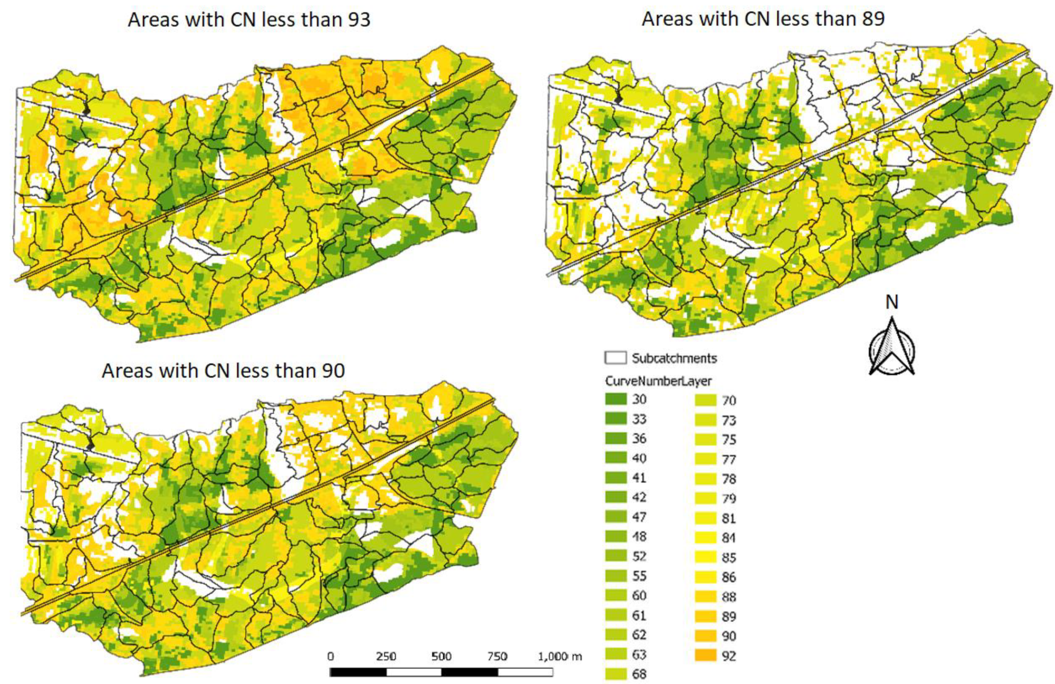
- Rather than classifying pervious/impervious areas, can CN values be used as a surrogate to determine whether an area can be considered impervious in SWMM? In other words, is there a threshold CN value that could determine whether a location is effectively impervious?
- (3)
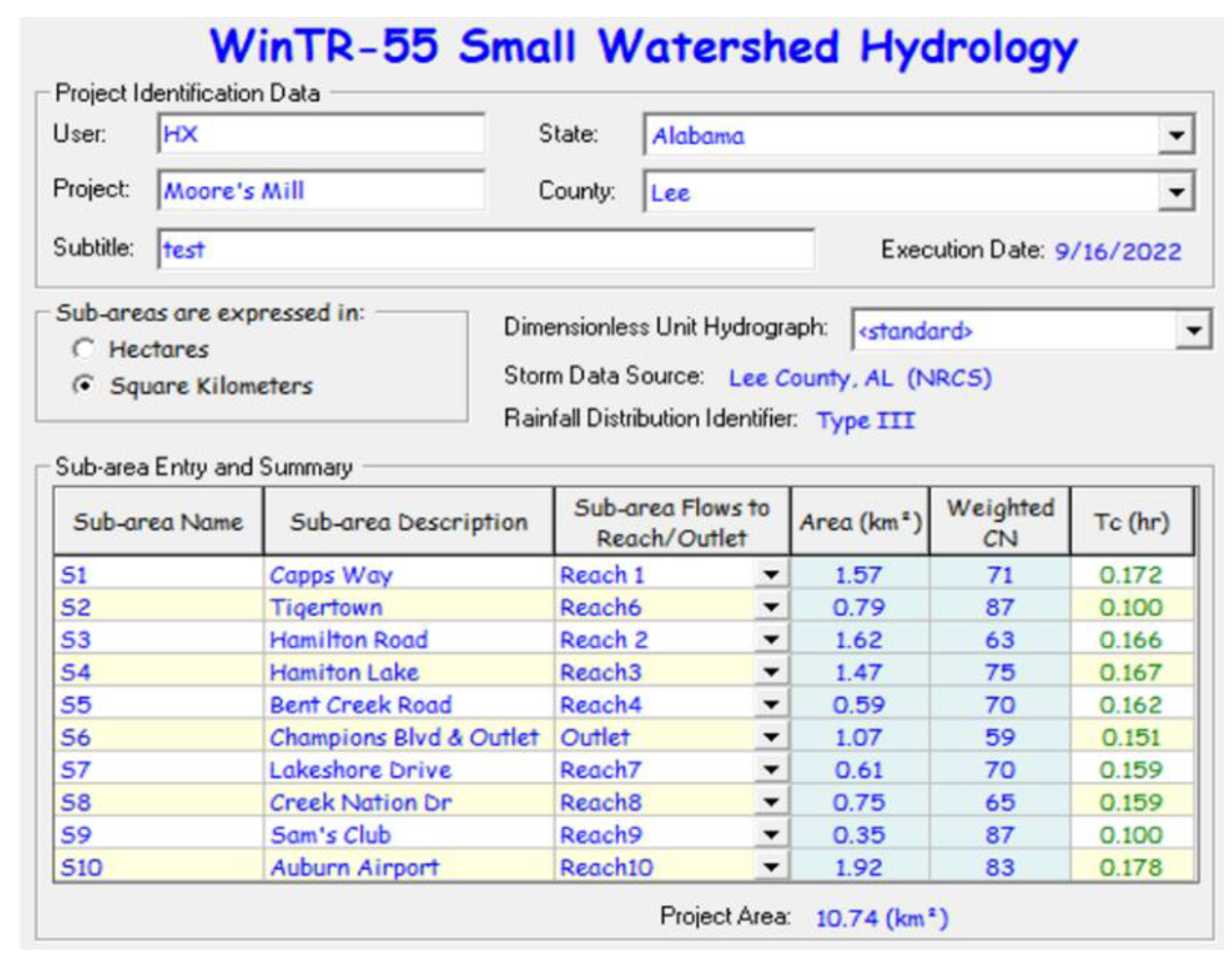
- For selected design storms, how do the predicted peak flows in SWMM compares with the corresponding peak flows yielded by WinTR-55 using the CN method?
2. Materials and Methods
2.1. Field Work
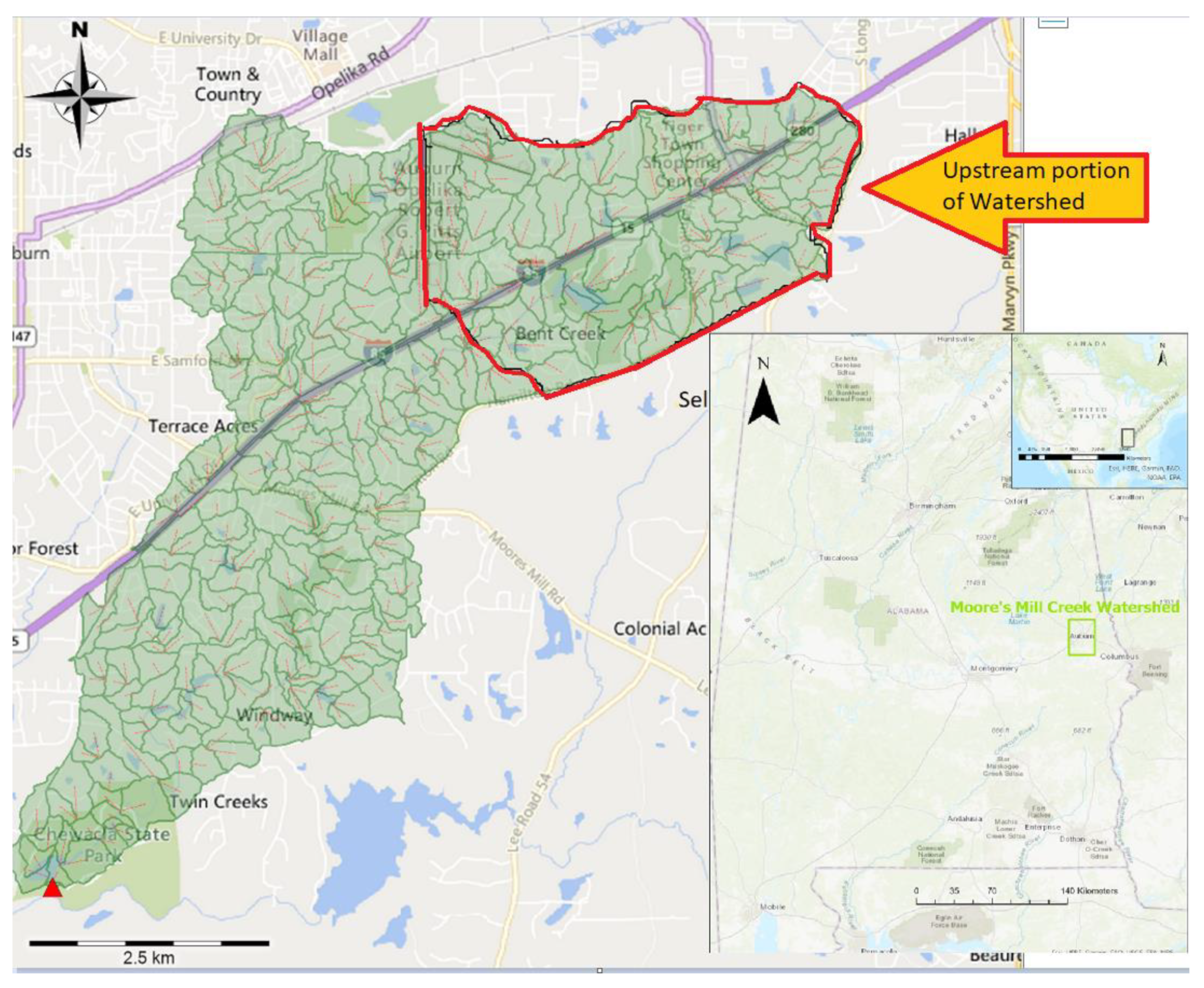
- Capps Way is the sub-watershed most upstream and is the headwaters of Moore’s Mill Creek. The land use is mostly comprised of forested areas, with is some ponds, low-density residential and commercial land use.
- Hamilton Road is a sub-watershed located mid-point along the stretch of Moore’s Mill Creek studied in this work. It drains a large commercial area and includes some ponds and forested areas.
- Bent Creek Road is the sub-watershed located most downstream of the studied stretch of Moore’s Mill Creek. It adds more low-density residential areas and more ponds. A dam at Hamilton Lake, which is immediately upstream of Bent Creek Road, provides peak flow attenuation during intense storms.
- Lakeshore Drive sub-watershed is a tributary watershed north of Moore’s Mill Creek, primarily with forested areas, low-density residential areas, and a pond.
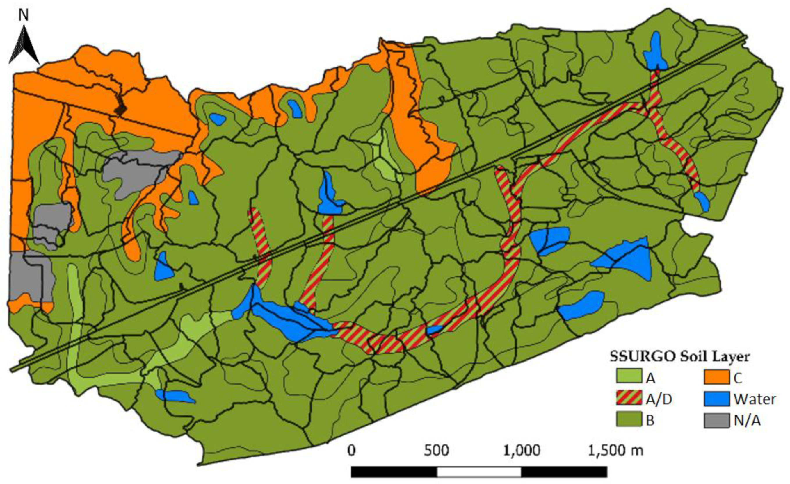
- Champions Boulevard sub-watershed is another tributary north to Moore’s Mill Creek, with mostly poorly drained soils, larger fraction of impervious areas due to a regional airport and commercial areas, and absence of ponds.
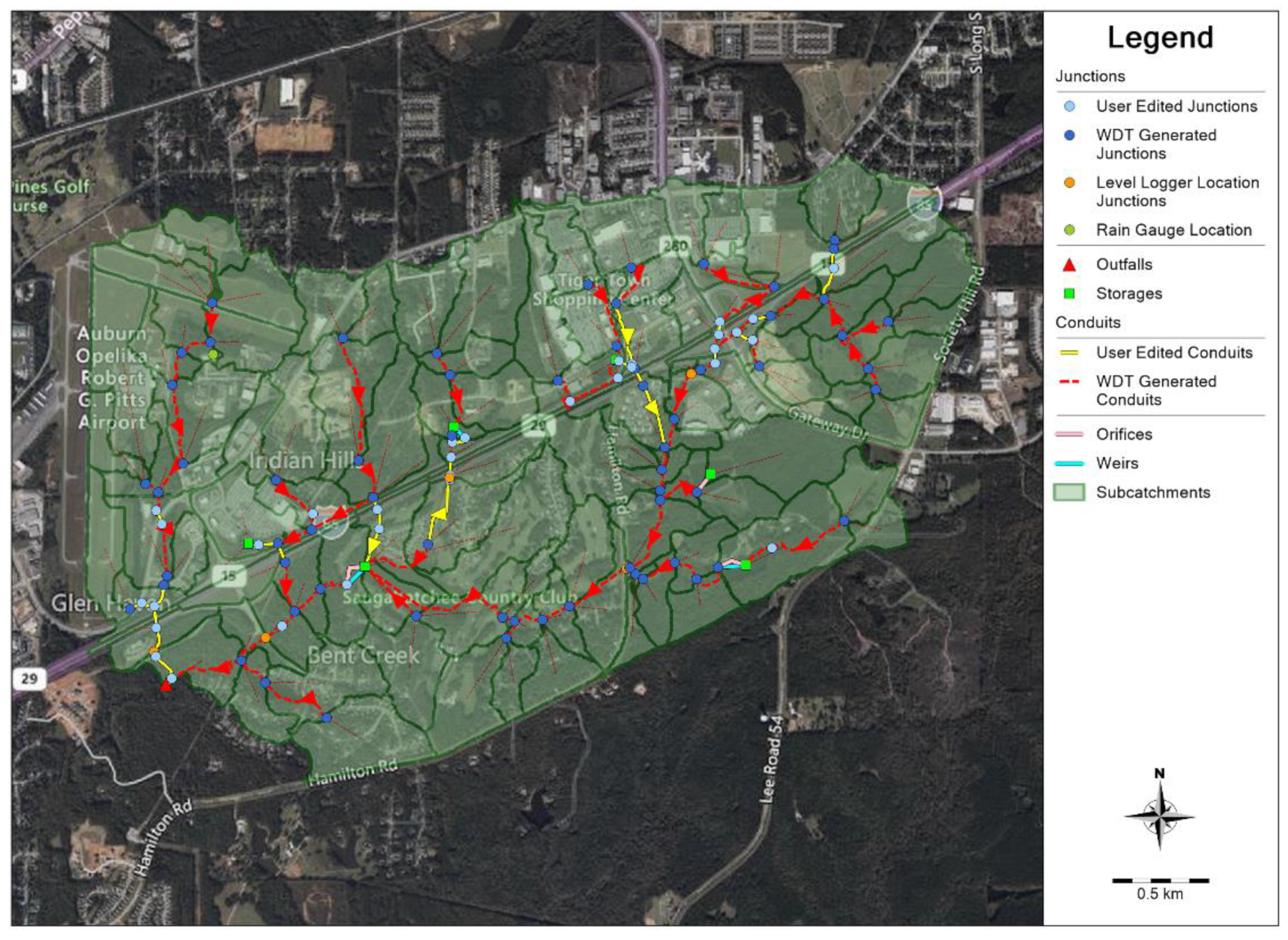
2.2. Numerical Modeling
3. Results and Discussion
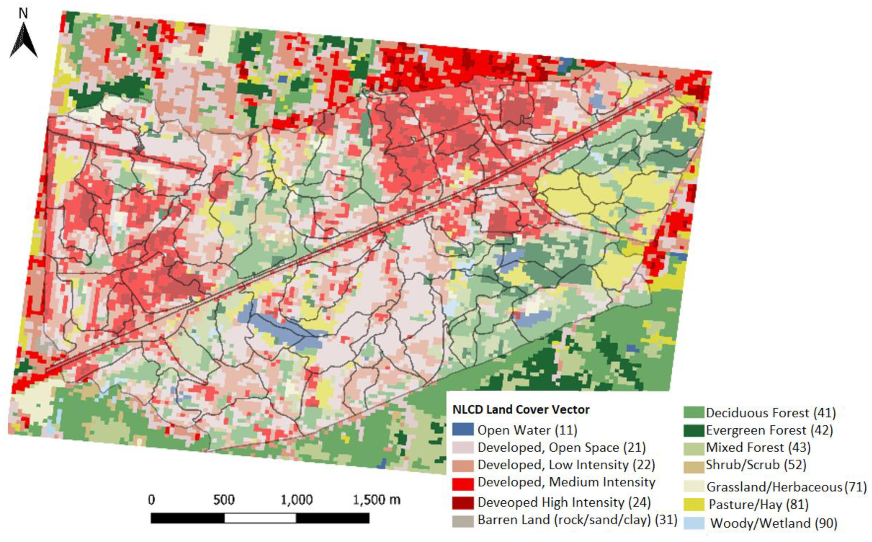
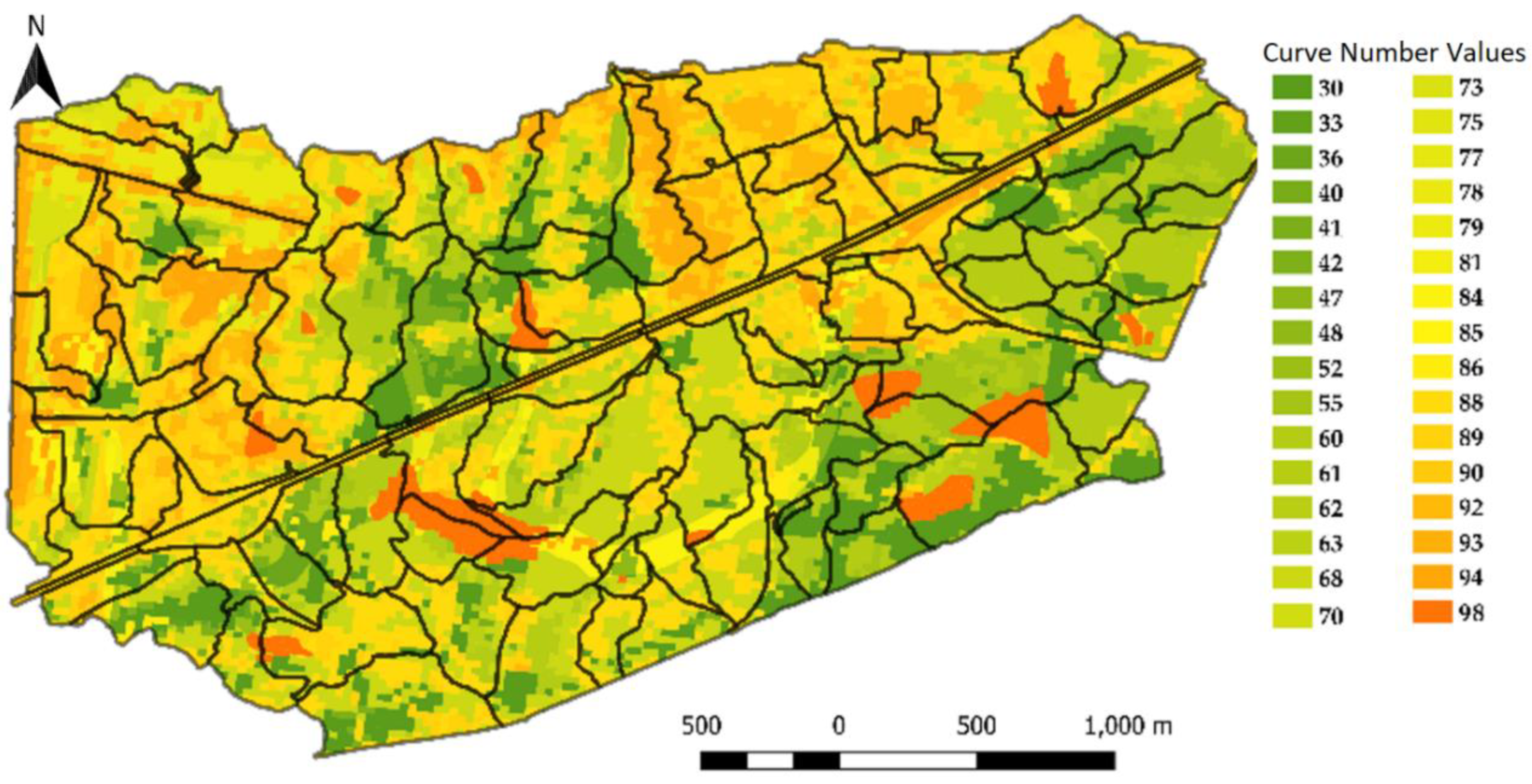
3.1. Watershed Properties and Resulting CN Values
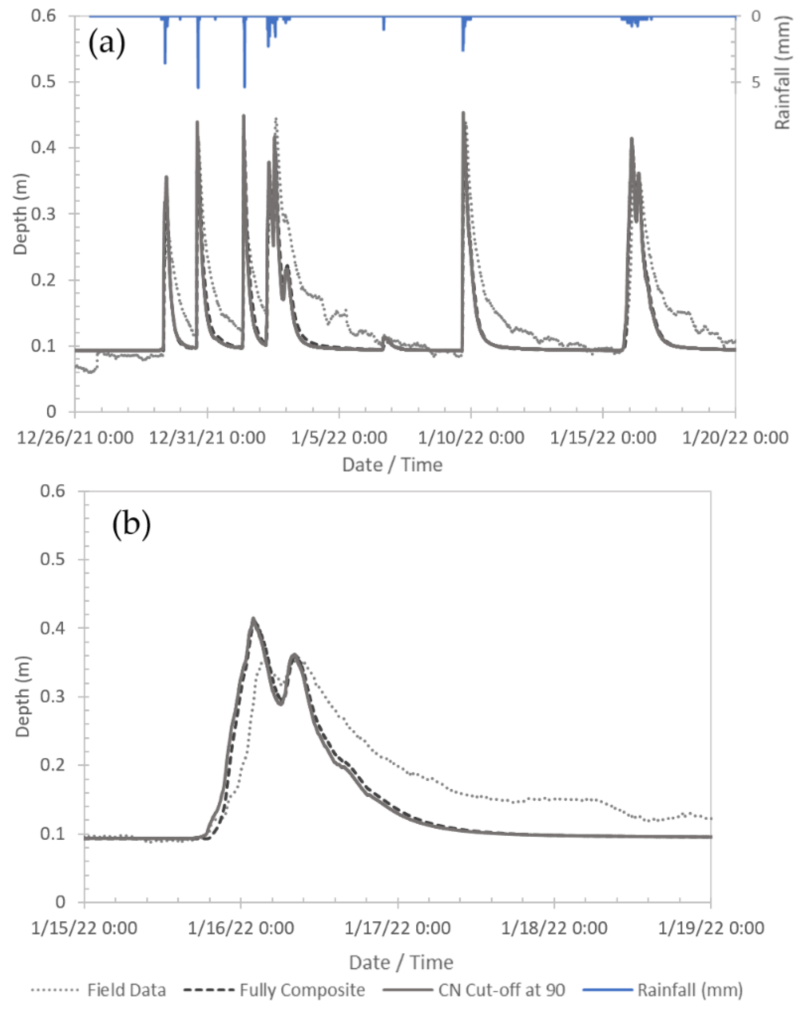
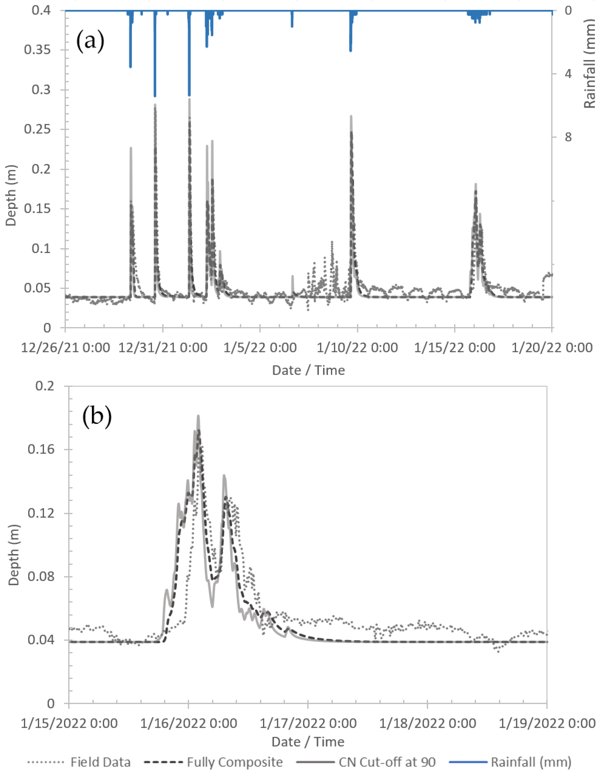
3.2. Flow Depth Hydrograph Results and Discussion
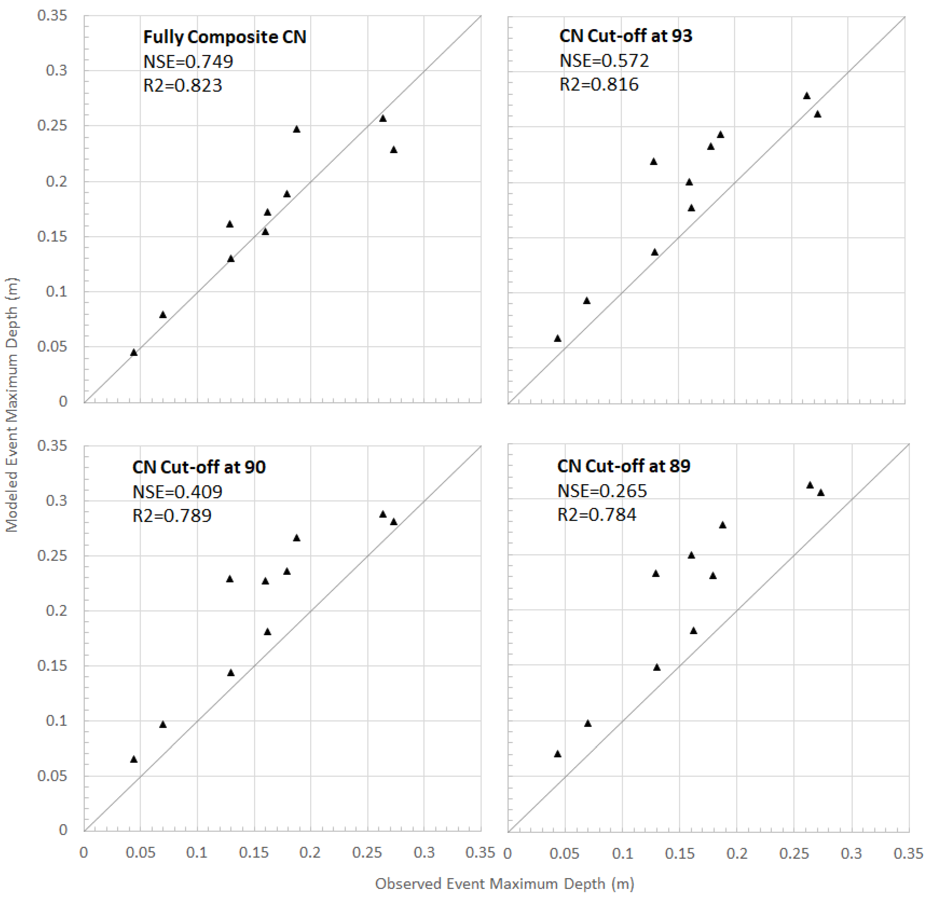
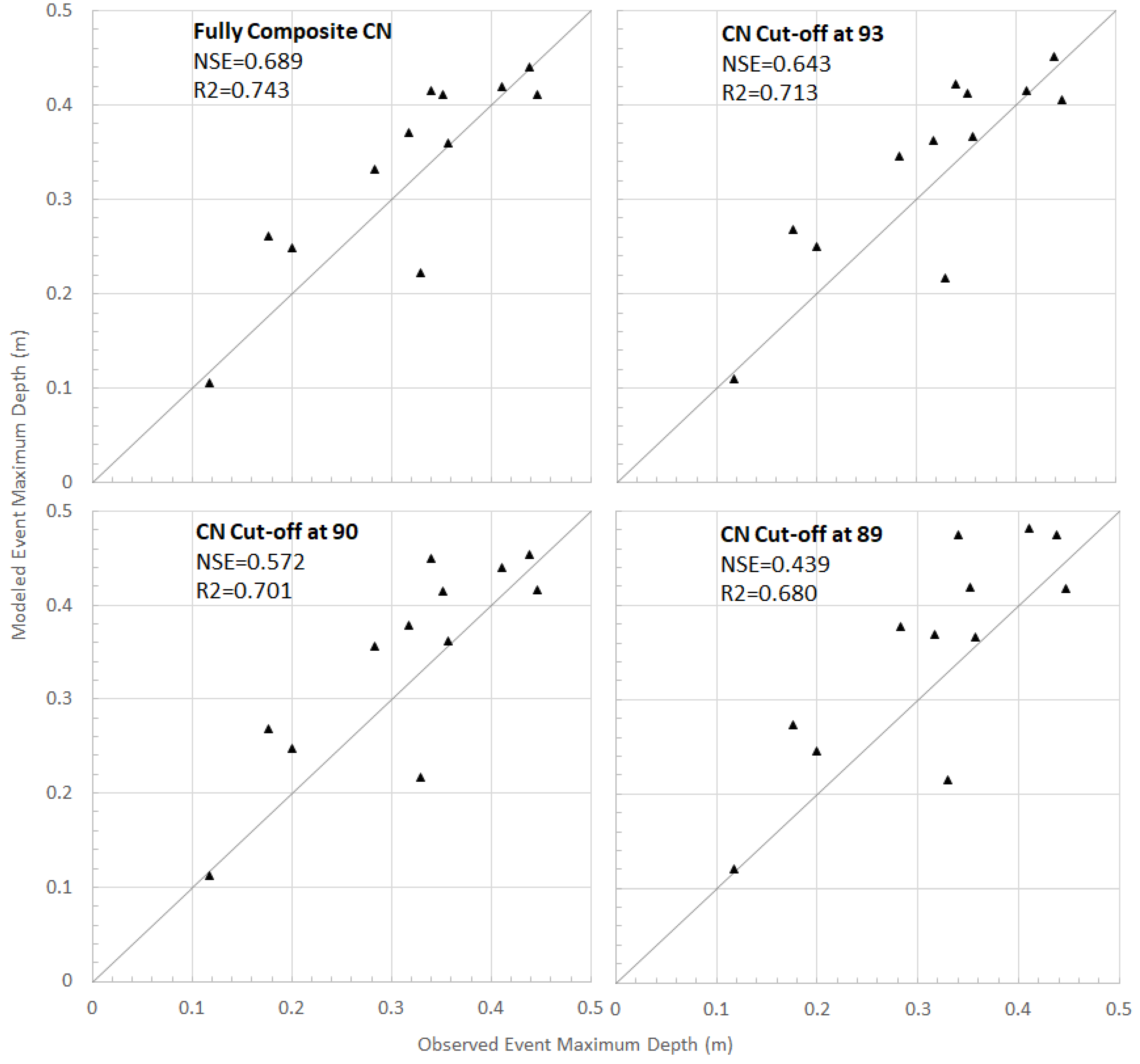
3.3. Peak Flow Depth Results and Discussion
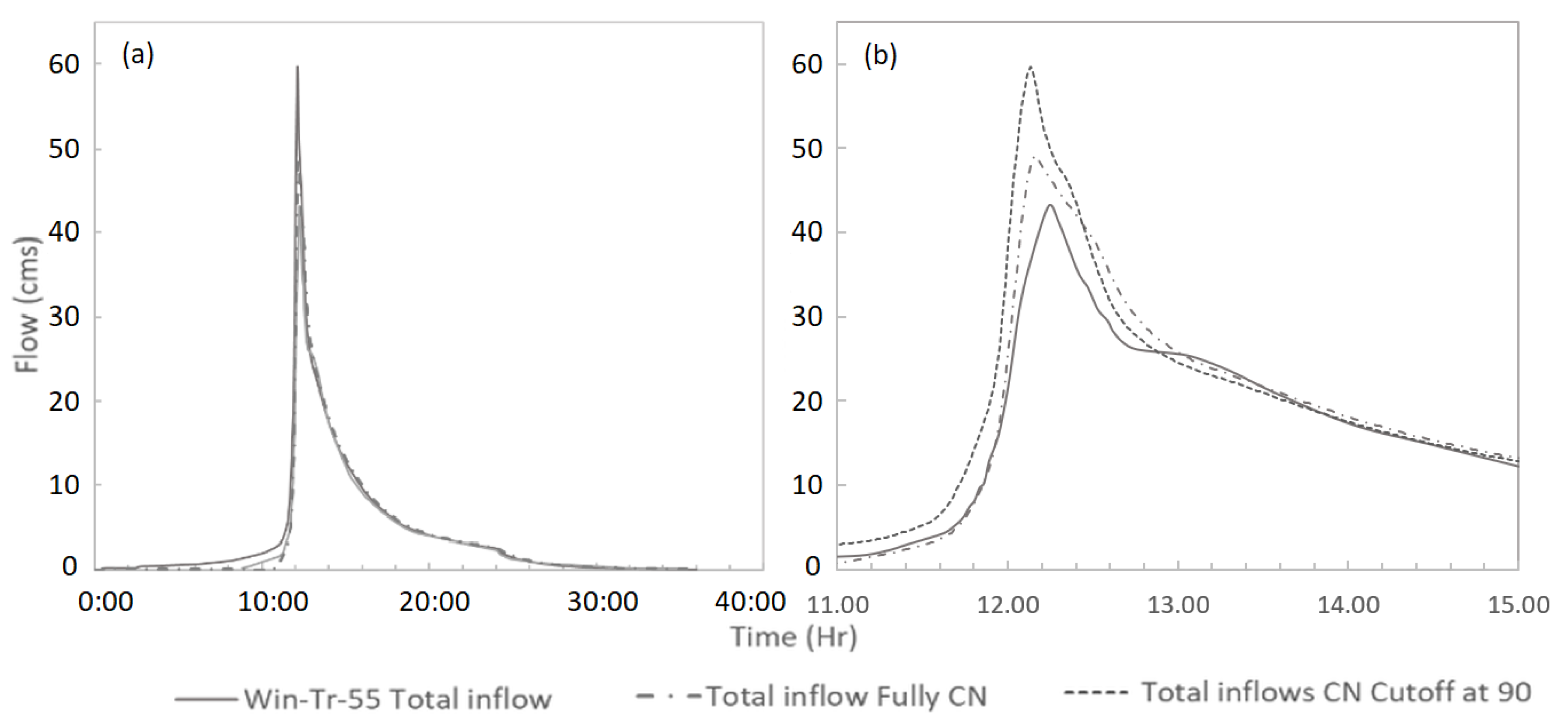
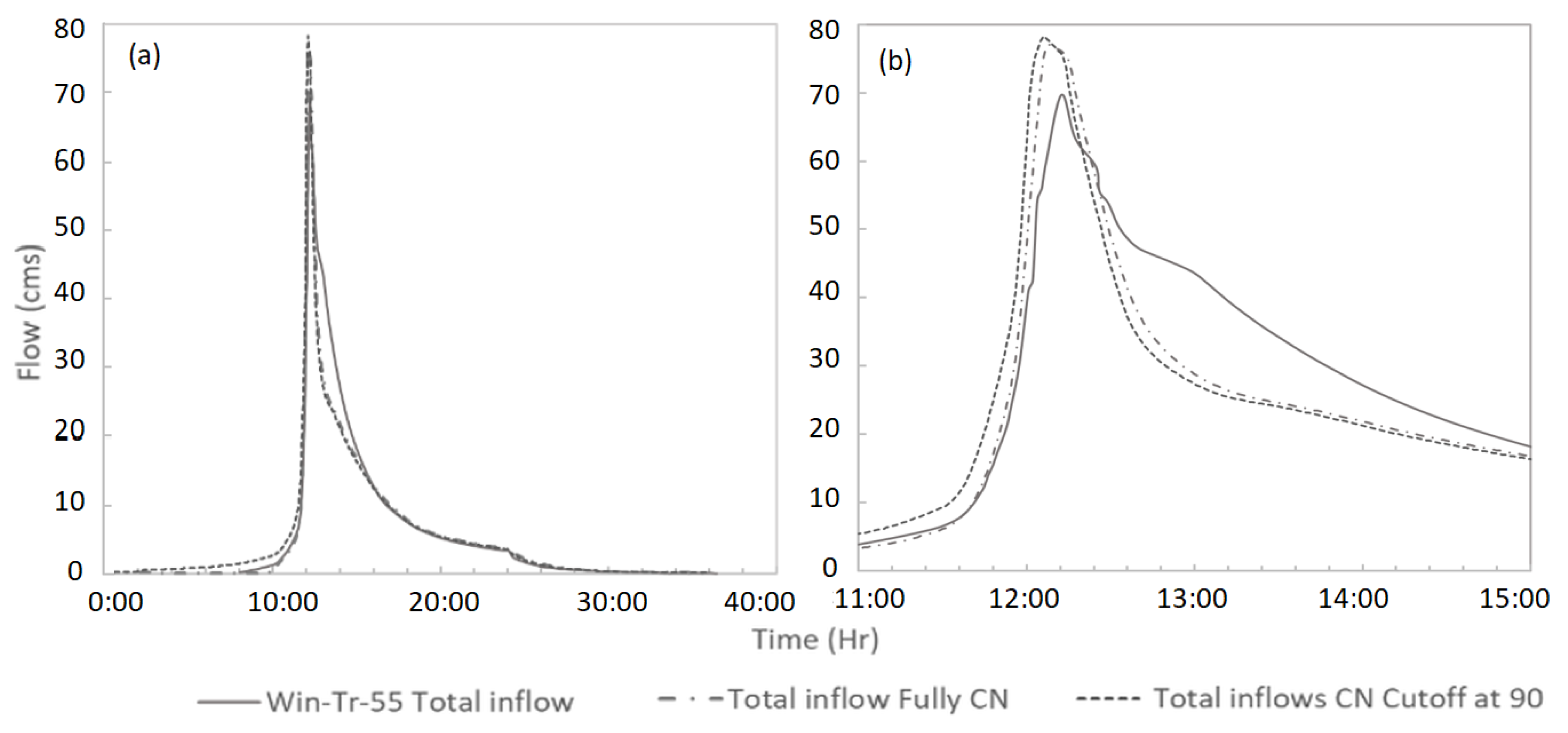
3.4. Flow Hydrograph Comparison between WinTR-55 and SWMM 5 Models
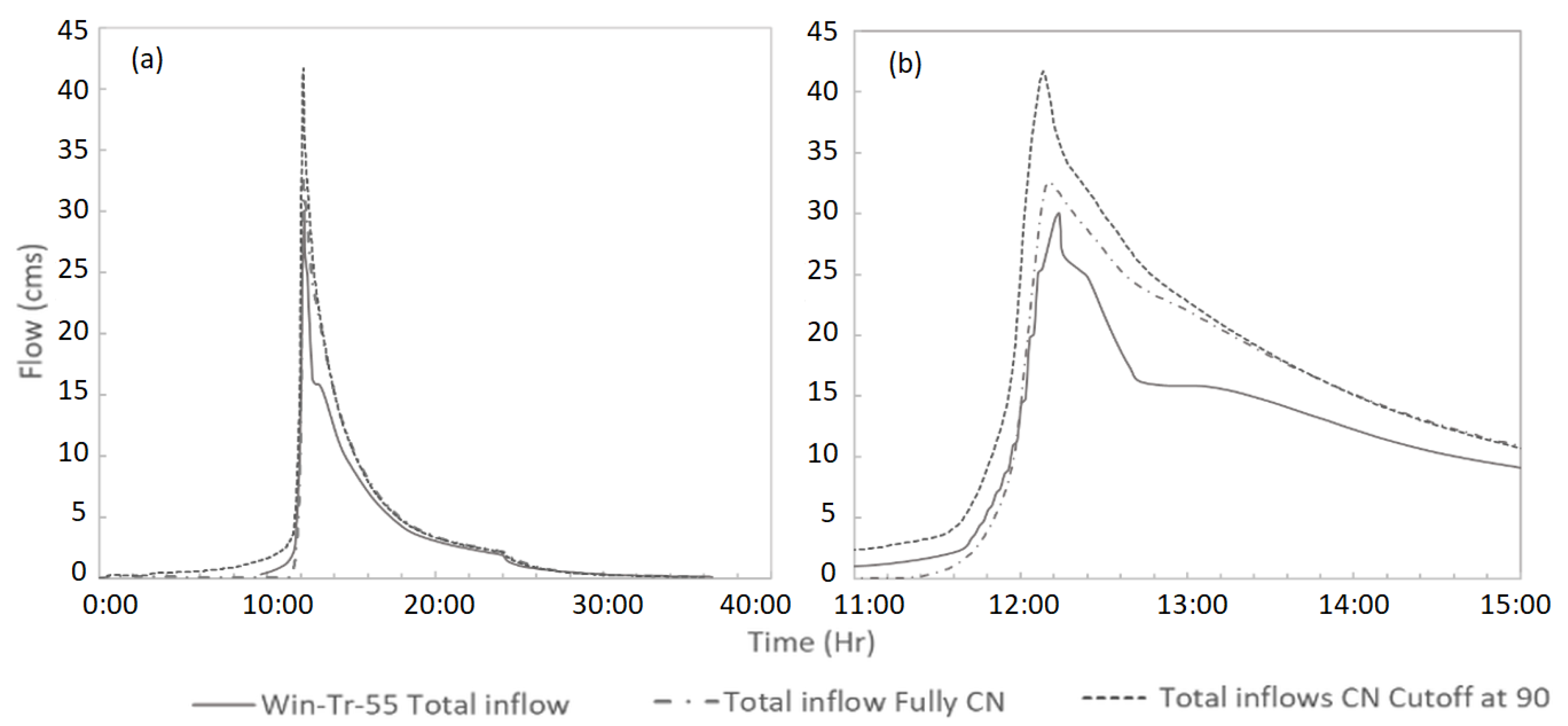
- As would be anticipated, SWMM modeling results from the Fully Composite approach are consistently closer to the flow hydrographs yielded by WinTR-55. However, this agreement decreased with the more intense rain events.
- WinTR-55 peak flow results were consistently smaller than SWMM modeling results.
- The CN Cut-off 90 and the Fully Composite approach agreement increased for higher intensity rain events. However, the CN Cut-off consistently had higher peak flows than the Fully Composite approach.
- Finally, the relative discrepancy between the model results decreased steadily with larger intensity rain events.


3.5. Summary of the Findings and Discussion
4. Conclusions and Recommendations for Future Work
Author Contributions
Funding
Data Availability Statement
Acknowledgments
Conflicts of Interest
References
- Feldman, A.D. Hydrologic Modeling System HEC-HMS Technical Reference Manual; U.S. Army Corps of Engineers Hydrologic Engineering Center, HEC: Davis, CA, USA, 2000; pp. 1–3. [Google Scholar]
- Rossman, L.A. Storm Water Management Model User’s Manual Version 5.1; U.S. Environmental Protection Agency, National Risk Management Research Laboratory Office of Research and Development: Cincinnati, OH, USA, 2015; pp. 12–13. [Google Scholar]
- NRCS. Small Watershed Hydrology WinTR-55 User Guide; United States Department of Agriculture: Washington, DC, USA, 2009. [Google Scholar]
- Rossman, L.A. Storm Water Management Model Reference Manual; Volume I—Hydrology (Revised); National Risk Management Laboratory Office of Research and Development U.S. Environmental Protection Agency: Cincinnati, OH, USA, 2016; pp. 86–87. [Google Scholar]
- Horton, R.E. The Role of Infiltration in the Hydrologic Cycle. Trans. Am. Geophys. Union 1933, 14, 446–460. [Google Scholar] [CrossRef]
- Green, W.H.; Ampt, G.A. Studies on Soil Physics, 1. The Flow of Air and Water Through Soils. J. Agric. Sci. 1911, 4, 11–24. [Google Scholar]
- NRCS. Urban Hydrology for Small Watersheds: TR-55; U.S. Department of Agriculture: Washington, DC, USA, 1986. [Google Scholar]
- Dao, D.A.; Kim, D.; Tran, D.H.H. Estimation of rainfall threshold for flood warning for small urban watersheds based on the 1D–2D drainage model simulation. Stoch. Environ. Res. Risk Assess. 2021, 36, 735–752. [Google Scholar] [CrossRef]
- Custodio, D.A.; Ghisi, E. Impact of residential rainwater harvesting on stormwater runoff. J. Environ. Manag. 2022, 326, 116814. [Google Scholar] [CrossRef] [PubMed]
- Prokešová, R.; Horáčková, Š.; Snopková, Z. Surface runoff response to long-term land use changes: Spatial rearrangement of runoff-generating areas reveals a shift in flash flood drivers. Sci. Total Environ. 2021, 815, 151591. [Google Scholar] [CrossRef] [PubMed]
- Barbero, G.; Costabile, P.; Costanzo, C.; Ferraro, D.; Petaccia, G. 2D hydrodynamic approach supporting evaluations of hydrological response in small watersheds: Implications for lag time estimation. J. Hydrol. 2022, 610, 127870. [Google Scholar] [CrossRef]
- Dao, D.A.; Kim, D.; Kim, S.; Park, J. Determination of flood-inducing rainfall and runoff for highly urbanized area based on high-resolution radar-gauge composite rainfall data and flooded area GIS data. J. Hydrol. 2020, 584, 124704. [Google Scholar] [CrossRef]
- Garen, D.C.; Moore, D.S. Curve Number Hydrology in Water Quality Modeling: Uses, Abuses, and Future Directions. J. Am. Water Resour. Assoc. 2005, 41, 377–378. [Google Scholar] [CrossRef]
- Praskievicz, S.; Chang, H. A review of hydrological modelling of basin-scale climate change and urban development impacts. Prog. Phys. Geogr. 2009, 33, 650–671. [Google Scholar] [CrossRef]
- Yan, H.; Edwards, F.G. Effects of Land Use Change on Hydrologic Response at a Watershed Scale, Arkansas. J. Hydrol. Eng. 2013, 18, 1779–1785. [Google Scholar] [CrossRef]
- Hawkins, R.H.; Ward, T.J.; Woodward, D.E.; Mullem, J.A.V. Curve Number Hydrology; Environmental and Water Resources Institute (EWRI) of the American Society of Civil Engineers: Reston, VA, USA, 2009. [Google Scholar]
- Hawkins, R.H.; Theurer, F.D.; Rezaeianzadeh, M. Understanding the Basis of the Curve Number Method for Watershed Models and TMDLs. J. Hydrol. Eng. 2019, 24, 06019003. [Google Scholar] [CrossRef]
- Galbetti, M.V.; Zuffo, A.C.; Shinma, T.A.; Boulomytis, V.T.G.; Imteaz, M. Evaluation of the tabulated, NEH4, least squares and asymptotic fitting methods for the CN estimation of urban watersheds. Urban Water J. 2022, 19, 244–255. [Google Scholar] [CrossRef]
- Bartlett MSParolari, A.J.; McDonnell, J.J.; Porporato, A. Beyond the SCS-CN method: A theoretical frameworkfor spatially lumped rainfall-runoff response. Water Resour. Res. 2016, 52, 4608–4627. [Google Scholar] [CrossRef] [Green Version]
- Hawkins, R.H. The importance of accurate curve numbers in the estimation of storm runoff. Water Resour. Bull. Am. Water Resour. Assoc. 1975, 11, 887–890. [Google Scholar] [CrossRef]
- USGS. National Land Cover Database (NLCD) 2019 Products (version 2.0, June 2021); U.S. Geological Survey data release: Reston, VA, USA, 2021. [Google Scholar] [CrossRef]
- USDA. Soil Survey Geographic Database (SSURGO). 2015. Available online: https://data.nal.usda.gov/dataset/soil-survey-geographic-database-ssurgo (accessed on 1 September 2022).
- Schoenfelder, C.; Kacvinsky, G.; Rossman, L. Open SWMM: Curve Number Assignment. 2007. Available online: https://www.openswmm.org/Topic/3481/curve-number-assignment (accessed on 10 October 2022).
- Zhang, G.; Dickinson, R.; Rovak, G.; Rossman, L. Open SWMM: Runoff Calculation Using Curve Number. 2007. Available online: https://www.openswmm.org/Topic/3584/runoff-calculation-using-curve-number (accessed on 10 October 2022).
- Numan, U.; Dickinson, R. Curve Numbers vs. % Impervious. 2022. Available online: https://www.openswmm.org/Topic/32629/curve-numbers-vs-impervious (accessed on 10 October 2022).
- Siddiqui, A.R. Curve Number Generator: A QGIS Plugin to Generate Curve Number Layer from Land Use and Soil. 2020. Available online: https://github.com/ar-siddiqui/curve_number_generator (accessed on 1 May 2022).
- James, W. Rules for Responsible Modeling; Computional Hydraulics International (CHI): Guelph, ON, Canada, 2005. [Google Scholar]
- Acer Engineering LLC. Moore’s Mill Creek Watershed Management Plan, Lee County, Alabama; Acer Engineering LLC: Raleigh, NC, USA, 2008. [Google Scholar]
- HOBO® Data Logger. HOBO® U20L Water Level Logger (U20L-0x) Manual; Onset Computer Corperation: Bourne, MA, USA, 2022; Available online: https://www.onsetcomp.com/datasheet/U20L-04 (accessed on 1 September 2021).
- HOBO Data Logging Rain Gauge (RG3 and RG3-M) Manual. Corporation, O.C., Ed. 2005–2018. Available online: https://www.onsetcomp.com/files/manual_pdfs/10241-M%20MAN-RG3%20and%20RG3-M.pdf (accessed on 1 September 2021).
- USDA. USDA Geospatial Data Gateway (GDG). Available online: https://datagateway.nrcs.usda.gov/ (accessed on 1 September 2021).
- Ries, K.G.; Guthrie, J.D.; Rea, A.H.; Steeves, P.A.; Stewart, D.W. StreamStats: A Water Resources Web Application; USGS Publicaitons Warehouse: Reston, VA, USA, 2008. [Google Scholar]
- UDFCD. Runoff. In Drainage Criteria Manual; Urban Drainage and Flood Control District: Dever, CO, USA, 2007; Chapter 5. [Google Scholar]
- ASCE. Gravity Sanitary Sewer Design and Construction; ASCE: New York, NY, USA, 1982. [Google Scholar]
- ASCE. Design & Construction of Urban Stormwater Management Systems; ASCE: New York, NY, USA, 1992. [Google Scholar]
- McCuen, R.E.A. Hydrology; Federal Highway Administration: Washington, DC, USA, 1996. [Google Scholar]
- Ormsbee, L.; Hoagland, S.; Peterson, K. Limitations of TR-55 Curve Numbers for Urban Development Applications: Critical Review and Potential Strategies for Moving Forward. J. Hydrol. Eng. 2020, 25, 02520001. [Google Scholar] [CrossRef]
- Alfredo, K.; Montalto, F.; Goldstein, A. Observed and Modeled Performances of Prototype Green Roof Test Plots Subjected to Simulated Low- and High-Intensity Precipitations in a Laboratory Experiment. J. Hydrol. Eng. 2010, 15, 444–457. [Google Scholar] [CrossRef]
- Swathi, V.; Raju, K.S.; Varma, M.R.R.; Veena, S.S. Automatic calibration of SWMM using NSGA-III and the effects of delineation scale on an urban catchment. J. Hydroinform. 2019, 21, 781–797. [Google Scholar] [CrossRef]
- Moriasi, D.N.; Arnold, J.G.; Liew, M.W.V.; Bingner, R.L.; Harmel, R.D.; Veith, T.L. Model Evaluation Guidelines for Systematic Quantification of Accuracy in Watershed Simulations. Am. Soc. Agric. Biol. Eng. 2007, 50, 885–900. [Google Scholar]
- Moriasi, D.N.; Gitau, M.W.; Pai, N.; Daggupati, P. Hydrologic and Water Quality Models: Performance Measures and Evaluation Criteria. Am. Soc. Agric. Biol. Eng. 2015, 58, 1763–1785. [Google Scholar] [CrossRef]
- U.S. Geological Survey. The StreamStats Program. 2019. Available online: https://streamstats.usgs.gov/ss/ (accessed on 1 August 2022).


| Surface | Manning’s n |
|---|---|
| Paved areas | 0.011 |
| Short prairie | 0.15 |
| Dense grass | 0.24 |
| Light wood underbrush | 0.4 |
| Dense wood underbrush | 0.8 |
| Method | No. of Pervious Features | No. of Impervious Features | Percent of Pervious Features |
|---|---|---|---|
| Fully Composite | 2430 | 0 | 100.0 |
| CN ≤ 98 | 2308 | 122 | 95.0 |
| 94 < CN < 98 | 2308 | 122 | 95.0 |
| CN < 93 | 2097 | 333 | 86.3 |
| 91 < CN < 92 | 1969 | 461 | 81.0 |
| CN < 90 | 1886 | 544 | 77.6 |
| CN < 89 | 1595 | 835 | 65.6 |
| CN < 88 | 1175 | 1255 | 48.4 |
| Sub-Watershed | Approach Used for CN Computation | |||
|---|---|---|---|---|
| StreamStats | CN Cut-Off 93 | CN Cut-Off 90 | CN Cut-Off 89 | |
| Capps Way | 21.1 | 5.2 | 13.3 | 28.1 |
| Hamilton Road | 21.0 | 9.6 | 17.4 | 31.4 |
| Bent Creek Road | 17.8 | 8.8 | 15.3 | 26.2 |
| Lakeshore Drive | 14.6 | 10.3 | 15.1 | 24.3 |
| Champions Blvd | 28.0 | 22.7 | 34.0 | 46.1 |
| Sub-Watershed | Area (km2) | Approach Used for CN Computation | |||
|---|---|---|---|---|---|
| Fully Composite | CN Cut-Off 93 | CN Cut-Off 90 | CN Cut-Off 89 | ||
| Capps Way | 1.667 | 74 | 71 | 70 | 68 |
| Hamilton Road | 3.945 | 72 | 69 | 68 | 66 |
| Bent Creek Road | 7.641 | 72 | 70 | 69 | 67 |
| Lakeshore Drive | 0.713 | 71 | 68 | 66 | 64 |
| Champions Blvd | 1.624 | 82 | 79 | 76 | 74 |
| Sub-Watershed | Approach Used for CN Computation | |||
|---|---|---|---|---|
| Fully Composite | CN Cut-Off at 93 | CN Cut-Off at 90 | CN Cut-Off at 89 | |
| Capps Way | 0.680 | 0.780 | 0.864 | 0.650 |
| Hamilton Road | 0.647 | 0.738 | 0.823 | 0.753 |
| Bent Creek Rd. | 0.689 | 0.643 | 0.572 | 0.439 |
| Lakeshore Dr. | 0.322 | 0.637 | 0.586 | 0.362 |
| Champions Blvd | 0.749 | 0.572 | 0.409 | 0.265 |
| Average NSE | 0.617 | 0.674 | 0.651 | 0.494 |
| Sub-Watershed | Approach Used for CN Computation | |||
|---|---|---|---|---|
| Fully Composite | CN Cut-Off at 93 | CN Cut-Off at 90 | CN Cut-Off at 89 | |
| Capps Way | 0.822 | 0.826 | 0.865 | 0.892 |
| Hamilton Road | 0.795 | 0.801 | 0.824 | 0.869 |
| Bent Creek Rd. | 0.743 | 0.713 | 0.701 | 0.680 |
| Lakeshore Dr. | 0.798 | 0.859 | 0.835 | 0.578 |
| Champions Blvd | 0.823 | 0.816 | 0.789 | 0.784 |
| Average R2 | 0.796 | 0.803 | 0.803 | 0.761 |
Disclaimer/Publisher’s Note: The statements, opinions and data contained in all publications are solely those of the individual author(s) and contributor(s) and not of MDPI and/or the editor(s). MDPI and/or the editor(s) disclaim responsibility for any injury to people or property resulting from any ideas, methods, instructions or products referred to in the content. |
© 2022 by the authors. Licensee MDPI, Basel, Switzerland. This article is an open access article distributed under the terms and conditions of the Creative Commons Attribution (CC BY) license (https://creativecommons.org/licenses/by/4.0/).
Share and Cite
Xiao, H.; Vasconcelos, J.G. Evaluating Curve Number Implementation Alternatives for Peak Flow Predictions in Urbanized Watersheds Using SWMM. Water 2023, 15, 41. https://doi.org/10.3390/w15010041
Xiao H, Vasconcelos JG. Evaluating Curve Number Implementation Alternatives for Peak Flow Predictions in Urbanized Watersheds Using SWMM. Water. 2023; 15(1):41. https://doi.org/10.3390/w15010041
Chicago/Turabian StyleXiao, Han, and Jose G. Vasconcelos. 2023. "Evaluating Curve Number Implementation Alternatives for Peak Flow Predictions in Urbanized Watersheds Using SWMM" Water 15, no. 1: 41. https://doi.org/10.3390/w15010041
APA StyleXiao, H., & Vasconcelos, J. G. (2023). Evaluating Curve Number Implementation Alternatives for Peak Flow Predictions in Urbanized Watersheds Using SWMM. Water, 15(1), 41. https://doi.org/10.3390/w15010041