
Multivariate Time Series Clustering of Groundwater Quality Data to Develop Data-Driven Monitoring Strategies in a Historically Contaminated Urban Area

 ,
,  ,
,  , and
, and
Abstract
1. Introduction
2. Materials and Methods
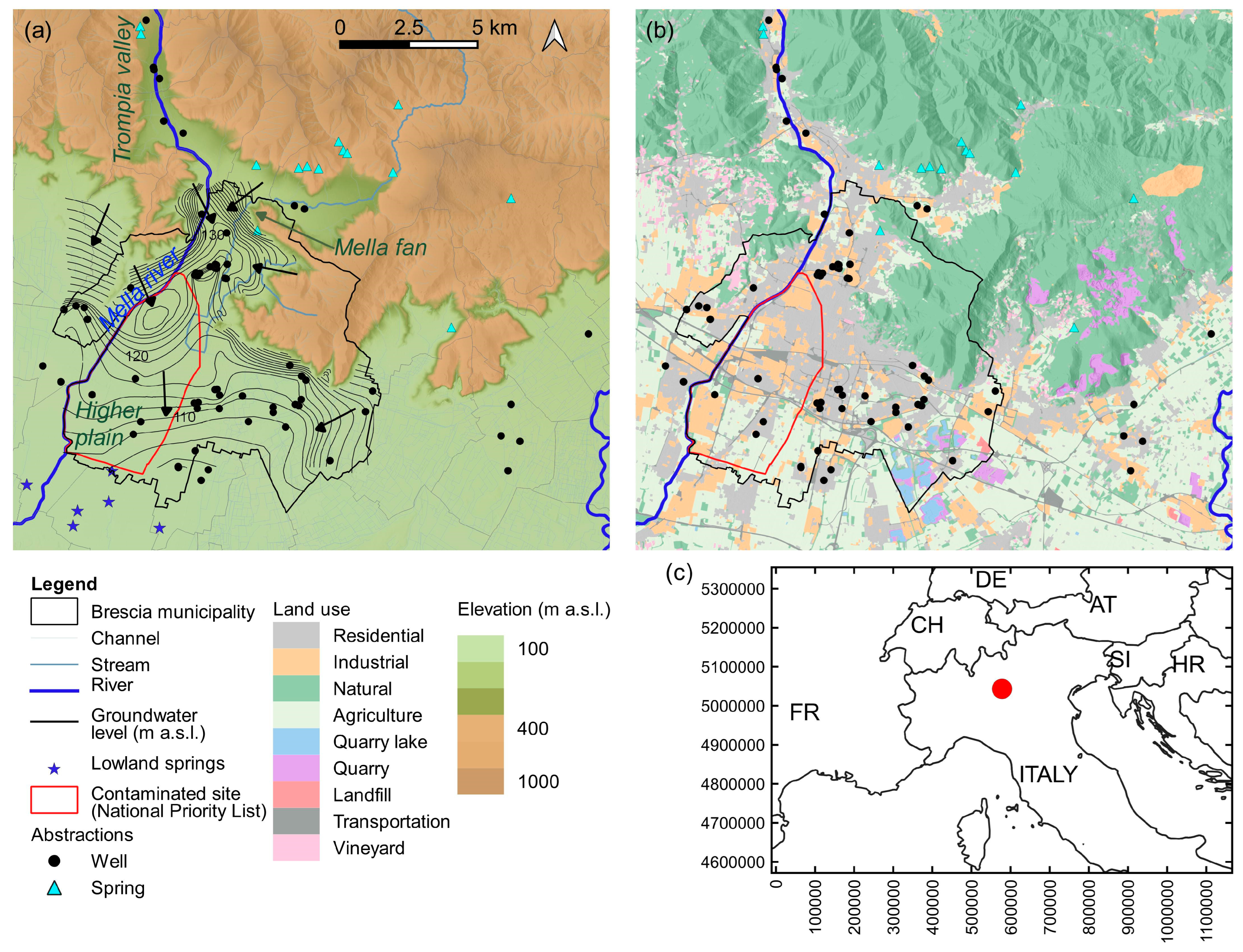
2.1. Study Area

2.2. Available Data
2.3. Data Analysis
2.3.1. Exploratory Analysis
2.3.2. Time Series Clustering
2.3.3. Development of Data-Driven Monitoring Strategies
- Increasing trends, which can be immediately considered as a warning situation. Therefore, immediate actions must be taken, and no indications for future warnings can be given.
- Decreasing trends, which indicate ongoing attenuation processes. For these wells any threshold value would be overestimated if based on the entire time series, while the early warning should be triggered if a peak or a new uptrend were to occur.
- Trends characterized by at least one changing point determining the trend inversion. For these cases, it is necessary to focus on the most recent part of the time series, identifying the current trend, which leads back to cases a and b.
3. Results and Discussion
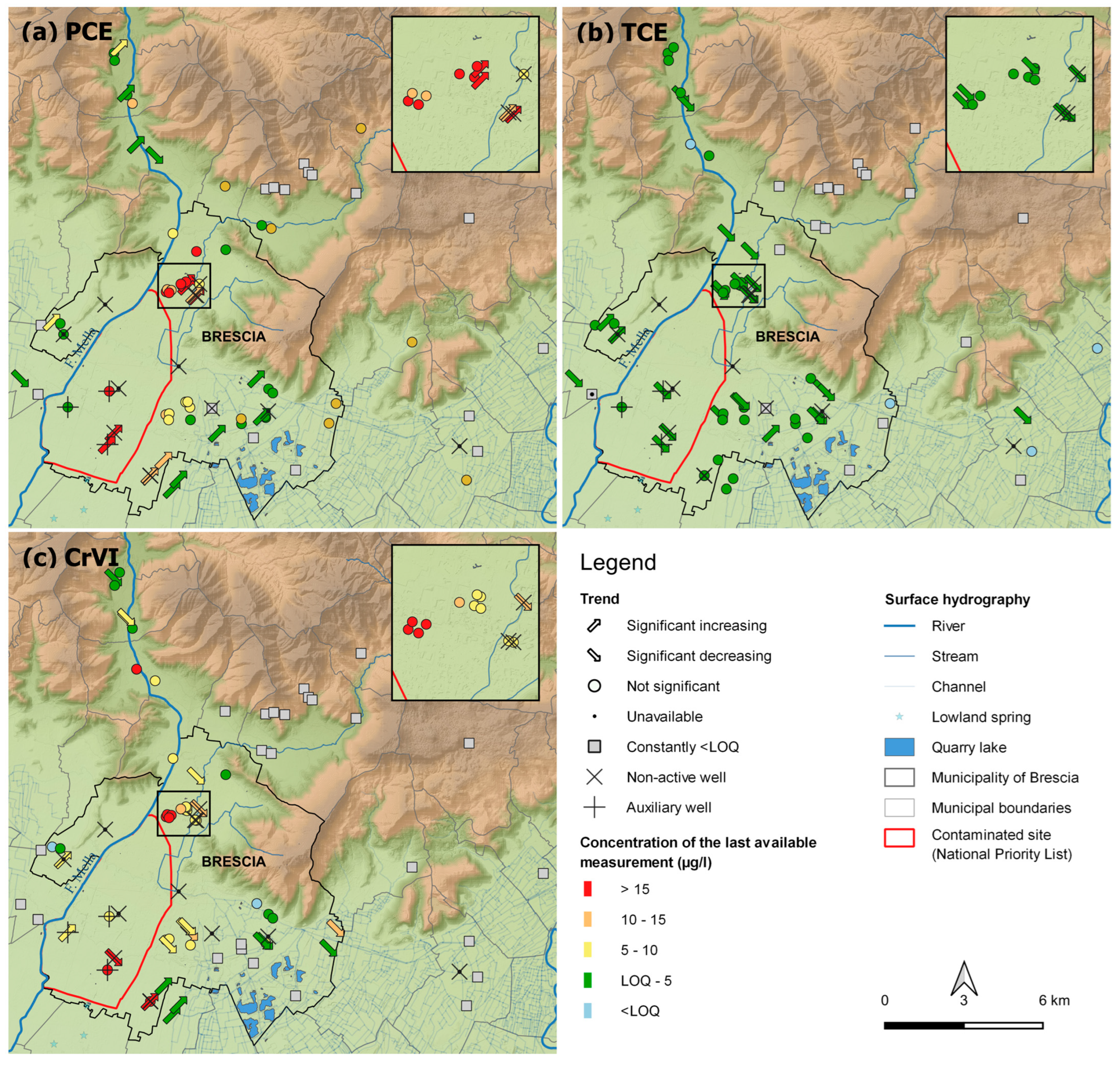
3.1. Exploratory Analysis
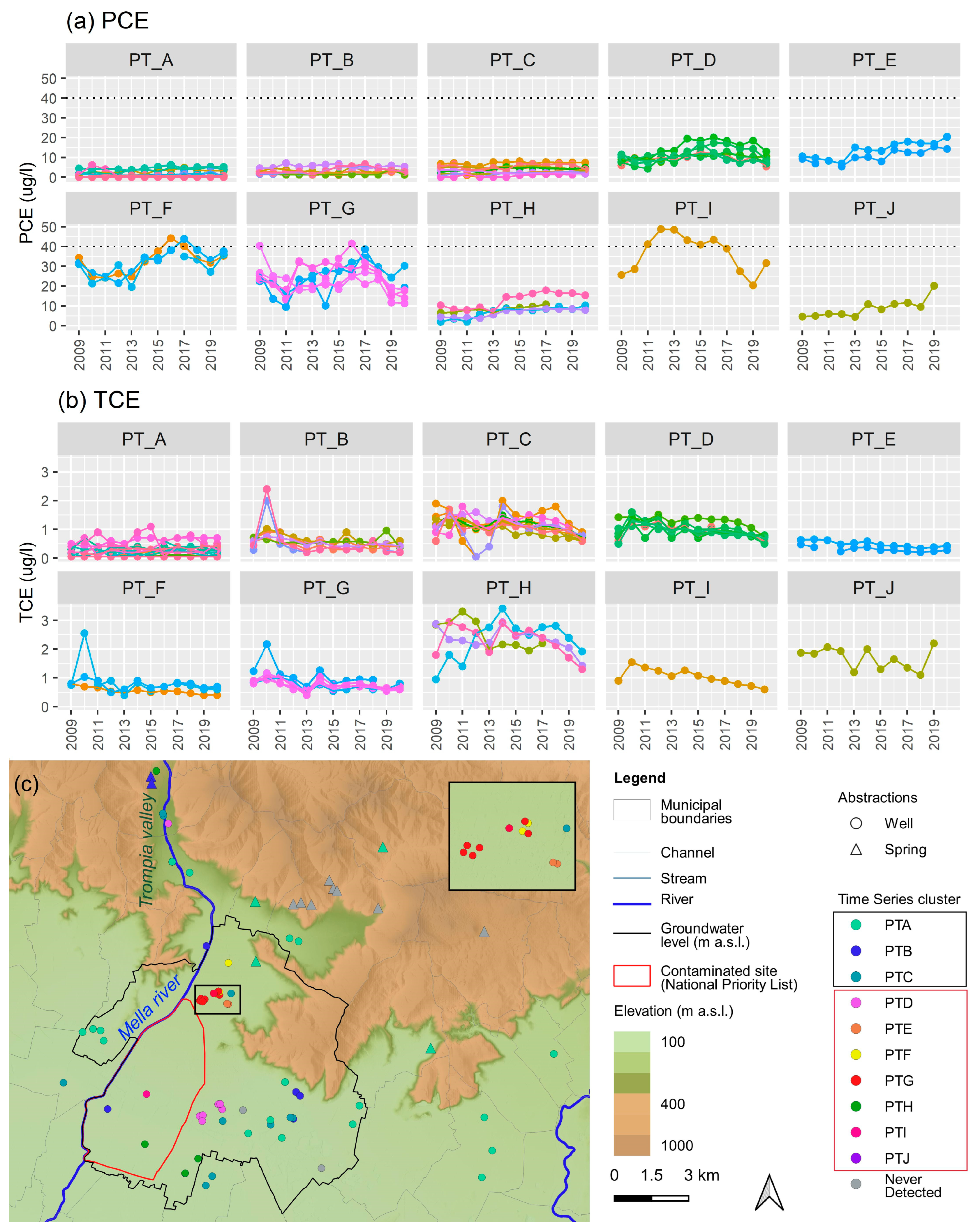
3.2. Time Series Clustering
3.2.1. Multivariate Time Series Clustering of PCE and TCE
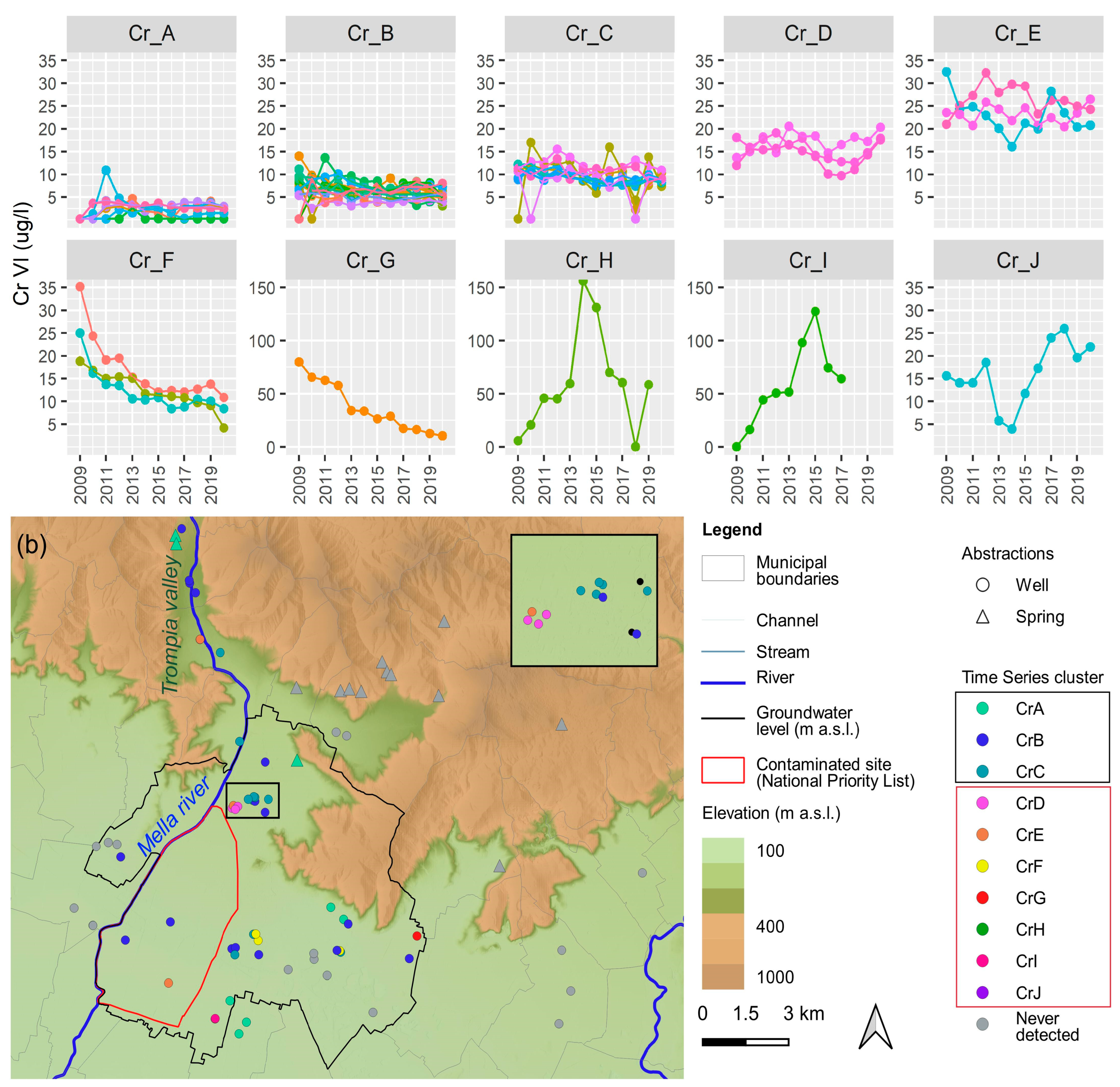
3.2.2. Univariate Time Series Clustering of Cr(VI)
3.3. Data-Driven Monitoring Strategies
3.4. Methodological Approach Pros and Cons
4. Conclusions
- Time series analysis of contamination data provides deep insights on the processes governing water quality, which would not be provided by the analysis of single field surveys
- Results of the exploratory analysis highlighted that the most common methods for trend analysis such as Mann-Kendall and Sen’s Slope could be non-exhaustive when dealing with highly variable groundwater chemical data since (a) they only work with monotonous trends and struggle with oscillatory behaviors and (b) they do not discriminate between lower and higher concentrations, focusing only on the trend’s shape while even increasing trends, over very low concentrations, can have scarce environmental relevance.
- Time series clustering overcame these issues and demonstrated to be an efficient tool for summarizing spatio-temporal variability of contamination data, allowing for an easier interpretation, and supporting the implementation of data-driven monitoring strategies
- The implementation of data-driven monitoring strategies can lead to more efficient, site-specific monitoring networks, able to avoid redundant analysis to focus on relevant or alarming trends.
Supplementary Materials
Author Contributions
Funding
Institutional Review Board Statement
Informed Consent Statement
Data Availability Statement
Acknowledgments
Conflicts of Interest
References
- UNESCO. The Role of Sound Groundwater Resource Management and Governance to Achieve Water Security; UNESCO: Paris, France; i-WSSM: Daejeon, Republic of Korea, 2021; ISBN 9789231004681. [Google Scholar]
- UNESCO. Water Security and the Sustainable Development Goals; UNESCO: Paris, France; i-WSSM: Daejeon, Republic of Korea, 2019; ISBN 9789231003233. [Google Scholar]
- United Nations. Water Development Report 2022: Groundwater: Making the Invisible Visible; United Nations: New York, NY, USA, 2022; ISBN 9789231005077. [Google Scholar]
- Zanotti, C.; Rotiroti, M.; Sterlacchini, S.; Cappellini, G.; Fumagalli, L.; Stefania, G.A.; Nannucci, M.S.; Leoni, B.; Bonomi, T. Choosing between Linear and Nonlinear Models and Avoiding Overfitting for Short and Long Term Groundwater Level Forecasting in a Linear System. J. Hydrol. 2019, 578, 124015. [Google Scholar] [CrossRef]
- Wunsch, A.; Liesch, T.; Broda, S. Forecasting Groundwater Levels Using Nonlinear Autoregressive Networks with Exogenous Input (NARX). J. Hydrol. 2018, 567, 743–758. [Google Scholar] [CrossRef]
- Bakker, M.; Schaars, F. Solving Groundwater Flow Problems with Time Series Analysis: You May Not Even Need Another Model. Groundwater 2019, 57, 826–833. [Google Scholar] [CrossRef] [PubMed]
- Giese, M.; Haaf, E.; Heudorfer, B.; Barthel, R. Comparative Hydrogeology–Reference Analysis of Groundwater Dynamics from Neighbouring Observation Wells. Hydrol. Sci. J. 2020, 65, 1685–1706. [Google Scholar] [CrossRef]
- Kayhomayoon, Z.; Milan, S.G.; Azar, N.A.; Kardan, H. A New Approach for Regional Groundwater Level Simulation: Clustering, Simulation, and Optimization. Nat. Resour. Res. 2021, 30, 4165–4185. [Google Scholar] [CrossRef]
- De Luca, D.A.; Destefanis, E.; Forno, M.G.; Lasagna, M.; Masciocco, L. The Genesis and the Hydrogeological Features of the Turin Po Plain Fontanili, Typical Lowland Springs in Northern Italy. Bull. Eng. Geol. Environ. 2014, 73, 409–427. [Google Scholar] [CrossRef]
- Frollini, E.; Preziosi, E.; Calace, N.; Guerra, M.; Guyennon, N.; Marcaccio, M.; Menichetti, S.; Romano, E.; Ghergo, S. Groundwater Quality Trend and Trend Reversal Assessment in the European Water Framework Directive Context: An Example with Nitrates in Italy. Environ. Sci. Pollut. Res. 2021, 28, 22092–22104. [Google Scholar] [CrossRef]
- Meggiorin, M.; Passadore, G.; Bertoldo, S.; Sottani, A.; Rinaldo, A. Assessing the Long-Term Sustainability of the Groundwater Resources in the Bacchiglione Basin (Veneto, Italy) with the Mann–Kendall Test: Suggestions for Higher Reliability. Acque Sotter. Ital. J. Groundw. 2021, 10, 35–48. [Google Scholar] [CrossRef]
- Egidio, E.; Lasagna, M.; Mancini, S.; De Luca, D.A. Climate Impact Assessment to the Groundwater Levels Based on Long Time-Series Analysis in a Paddy Field Area (Piedmont Region, NW Italy): Preliminary Results. Acque Sotter. Ital. J. Groundw. 2022, 11, 21–29. [Google Scholar] [CrossRef]
- Barbieri, M.; Franchini, S.; Barberio, M.D.; Billi, A.; Boschetti, T.; Giansante, L.; Gori, F.; Jónsson, S.; Petitta, M.; Skelton, A.; et al. Changes in Groundwater Trace Element Concentrations before Seismic and Volcanic Activities in Iceland during 2010–2018. Sci. Total Environ. 2021, 793, 148635. [Google Scholar] [CrossRef]
- Rai, P.; Singh, S. A Survey of Clustering Techniques. Int. J. Comput. Appl. 2010, 7, 1–5. [Google Scholar] [CrossRef]
- Aghabozorgi, S.; Seyed Shirkhorshidi, A.; Ying Wah, T. Time-Series Clustering—A Decade Review. Inf. Syst. 2015, 53, 16–38. [Google Scholar] [CrossRef]
- Kumar, R.; Nagabhushan, P. Time Series as a Point—A Novel Approach for Time Series Cluster Visualization. Conf. Data Min. 2006, 24–29. Available online: https://www.semanticscholar.org/paper/Time-Series-as-a-Point-A-Novel-Approach-for-Time-Kumar-Nagabhushan/507cc47a5d0954fd87591929c50974d96c93ad24 (accessed on 10 November 2022).
- Li, L.; Prakash, B.A. Time Series Clustering: Complex Is Simpler! 2011. Available online: https://www.pdl.cmu.edu/PDL-FTP/associated/li-icml11-time.pdf (accessed on 10 November 2022).
- Rani, S. Recent Techniques of Clustering of Time Series Data: A Survey. Int. J. Comput. Appl. 2012, 52, 1–9. [Google Scholar] [CrossRef]
- Caiado, J.; Maharaj, E.A.; D’Urso, P. Time Series Clustering. In Handbook of Cluster Analysis; Chapman and Hall/CRC: Boca Raton, FL, USA, 2015; pp. 241–263. [Google Scholar]
- Akay, Ö. Examination of the 21 European Countries and Turkey in Terms of Water Resources along with the Effect of Climate Change by Time Series Clustering. Environ. Earth Sci. 2021, 80, 784. [Google Scholar] [CrossRef]
- Utimula, K.; Hunkao, R.; Yano, M.; Kimoto, H.; Hongo, K.; Kawaguchi, S.; Suwanna, S.; Maezono, R. Machine-Learning Clustering Technique Applied to Powder X-Ray Diffraction Patterns to Distinguish Compositions of ThMn12-Type Alloys. Adv. Theory Simul. 2020, 3, 2000039. [Google Scholar] [CrossRef]
- Warren Liao, T. Clustering of Time Series Data—A Survey. Pattern Recognit. 2005, 38, 1857–1874. [Google Scholar] [CrossRef]
- Prakaisak, I.; Wongchaisuwat, P. Hydrological Time Series Clustering: A Case Study of Telemetry Stations in Thailand. Water 2022, 14, 2095. [Google Scholar] [CrossRef]
- Lee, W.; Zeyar, W.; Catalina, A.; Stuart, F.; Eds, M.; Goebel, R.; Arslan, Y.; Küçük, D.; Eren, S.; Birturk, A. Clustering River Basins Using Time-Series Data Mining on Hydroelectric Energy Generation. In Proceedings of the International Workshop on Data Analytics for Renewable Energy Integration, Dublin, Ireland, 10 September 2018; pp. 103–115. [Google Scholar]
- Mishra, S.; Saravanan, C.; Dwivedi, V.K.; Shukla, J.P. Rainfall-Runoff Modeling Using Clustering and Regression Analysis for the River Brahmaputra Basin. J. Geol. Soc. India 2018, 92, 305–312. [Google Scholar] [CrossRef]
- Sartirana, D.; Rotiroti, M.; Bonomi, T.; De Amicis, M.; Nava, V.; Fumagalli, L.; Zanotti, C. Data-Driven Decision Management of Urban Underground Infrastructure through Groundwater-Level Time-Series Cluster Analysis: The Case of Milan (Italy). Hydrogeol. J. 2022, 30, 1157–1177. [Google Scholar] [CrossRef]
- Naranjo-Fernández, N.; Guardiola-Albert, C.; Aguilera, H.; Serrano-Hidalgo, C.; Montero-González, E. Clustering Groundwater Level Time Series of the Exploited Almonte-Marismas Aquifer in Southwest Spain. Water 2020, 12, 1063. [Google Scholar] [CrossRef]
- Rinderer, M.; van Meerveld, H.J.; McGlynn, B.L. From Points to Patterns: Using Groundwater Time Series Clustering to Investigate Subsurface Hydrological Connectivity and Runoff Source Area Dynamics. Water Resour. Res. 2019, 55, 5784–5806. [Google Scholar] [CrossRef]
- Moghaddam, H.K.; Milan, S.G.; Kayhomayoon, Z.; Kivi, Z.R.; Azar, N.A. The Prediction of Aquifer Groundwater Level Based on Spatial Clustering Approach Using Machine Learning. Environ. Monit. Assess. 2021, 193, 173. [Google Scholar] [CrossRef] [PubMed]
- Huang, L.; Feng, H.; Le, Y. Finding Water Quality Trend Patterns Using Time Series Clustering: A Case Study. In Proceedings of the IEEE Fourth International Conference on Data Science in Cyberspace (DSC), Hangzhou, China, 23–25 June 2019; pp. 330–337. [Google Scholar] [CrossRef]
- Lee, S.; Kim, J.; Hwang, J.; Lee, E.J.; Lee, K.J.; Oh, J.; Park, J.; Heo, T.Y. Clustering of Time Series Water Quality Data Using Dynamic Time Warping: A Case Study from the Bukhan River Water Quality Monitoring Network. Water 2020, 12, 2411. [Google Scholar] [CrossRef]
- Pollicino, L.C.; Masetti, M.; Stevenazzi, S.; Colombo, L.; Alberti, L. Spatial Statistical Assessment of Groundwater PCE (Tetrachloroethylene) Diffuse Contamination in Urban Areas. Water 2019, 11, 1211. [Google Scholar] [CrossRef]
- Alberti, L.; Azzellino, A.; Colombo, L.; Lombi, S. Cluster Analysis to Identify Tetrachloroethylene Pollution Hotspots for Transport Numerical Model Implementation in Urban Functional Area of Milan, Italy. In Proceedings of the 16th International Multidisciplinary Scientific Conference SGEM2016, Albena, Bulgaria, 28 June–7 July 2016. Book 1. [Google Scholar]
- Azzellino, A.; Colombo, L.; Lombi, S.; Marchesi, V.; Piana, A.; Merri, A.; Alberti, L. Groundwater Diffuse Pollution in Functional Urban Areas: The Need to Define Anthropogenic Diffuse Pollution Background Levels. Sci. Total Environ. 2019, 656, 1207–1222. [Google Scholar] [CrossRef]
- Kottek, M.; Grieser, J.; Beck, C.; Rudolf, B.; Rubel, F. World Map of the Köppen-Geiger Climate Classification Updated. Meteorol. Z. 2006, 15, 259–263. [Google Scholar] [CrossRef]
- Francani, V. La Stato Di Inquinamento Delle Risorse Idriche Della Pianura Padana e Gli Interventi Possibili. In Studi Idrogeologici Sulla Pianura Padana; 1987; Available online: http://wwwdb.gndci.cnr.it/php2/gndci/gndci_f_regione.php?®ione=Italia+Settentrionale&inizio=50&formato=&lingua=en (accessed on 10 November 2022).
- Vercesi, P.L. Aspetti Quali-Quantitativi Delle Risorse Idriche Sotterranee Del Bresciano. Nat. Brescia 1994, 29, 21–52. [Google Scholar]
- Denti, E.; Lauzi, S.; Sala, P.; Scesi, L. Studio Idrogeologico Della Pianura Bresciana Tra i Fiumi Oglio e Chiese. In Studi Idrogeologici Sulla Pianura Padana; ERSAL: Milano, Italy, 1998. [Google Scholar]
- Gasparetti, D.; Tribani, M.; Ribolla, G.; Gavazzi, F.; Treccani, L. Adeguamento Della Componente Geologica, Idrogeologica e Sismica Del PGT Al Piano Di Gestione Del Rischio Alluvioni; 2009; Available online: https://www.comune.brescia.it/servizi/urbanistica/PGT/Pagine/pgt_approvazione_%20variante_idrogeologica.aspx (accessed on 10 November 2022).
- Osservatorio Acqua Bene Comune. Primo Rapporto; Osservatorio Acqua Bene Comune: Comune di Brescia, Brescia, 2015. [Google Scholar]
- ARPA—Lombardia. Attivita’ Di Affinamento Delle Conoscenze Sulla Contaminazionedelle Acque Sotterranee in Cinque Aree Della Provincia Di Brescia Con Definizione Dei Plumes Di Contaminanti Ed Individuazione Delle Potenziali Fonti Di Contaminazione—Area BS002—Brescia—C; ARPA: Milano, Italy, 2016.
- ARPA—Lombardia. Attivita’ Di Affinamento Delle Conoscenze Sulla Contaminazionedelle Acque Sotterranee in Cinque Aree Della Provincia Di Brescia Con Definizione Dei Plumes Di Contaminanti Ed Individuazione Delle Potenziali Fonti Di Contaminazione- Lotto A—Area BS001—F; ARPA: Milano, Italy, 2015.
- WHO. A Global Overview of National Regulations and Standards for Drinking-Water Quality. Second Edition; WHO: Geneva, Switzerland, 2021; ISBN 978-92-4-151376-0.
- European Commission. Guidance Document No. 18 Guidance on Groundwater Status and Trend Assessment; European Commission: Brussels, Belgium, 2009; ISBN 9789279113741.
- Mann, H.B. Nonparametric Tests Against Trend. Econometrica 1945, 13, 245–259. [Google Scholar] [CrossRef]
- Kendall, M.G. Rank Correlation Methods; Charles Griffin: London, UK, 1975. [Google Scholar]
- Sen, P.K. Estimates of the Regression Coefficient Based on Kendall’s Tau. J. Am. Stat. Assoc. 1968, 63, 1379–1389. [Google Scholar] [CrossRef]
- Almazroui, M.; Şen, Z. Trend Analyses Methodologies in Hydro-Meteorological Records. Earth Syst. Environ. 2020, 4, 713–738. [Google Scholar] [CrossRef]
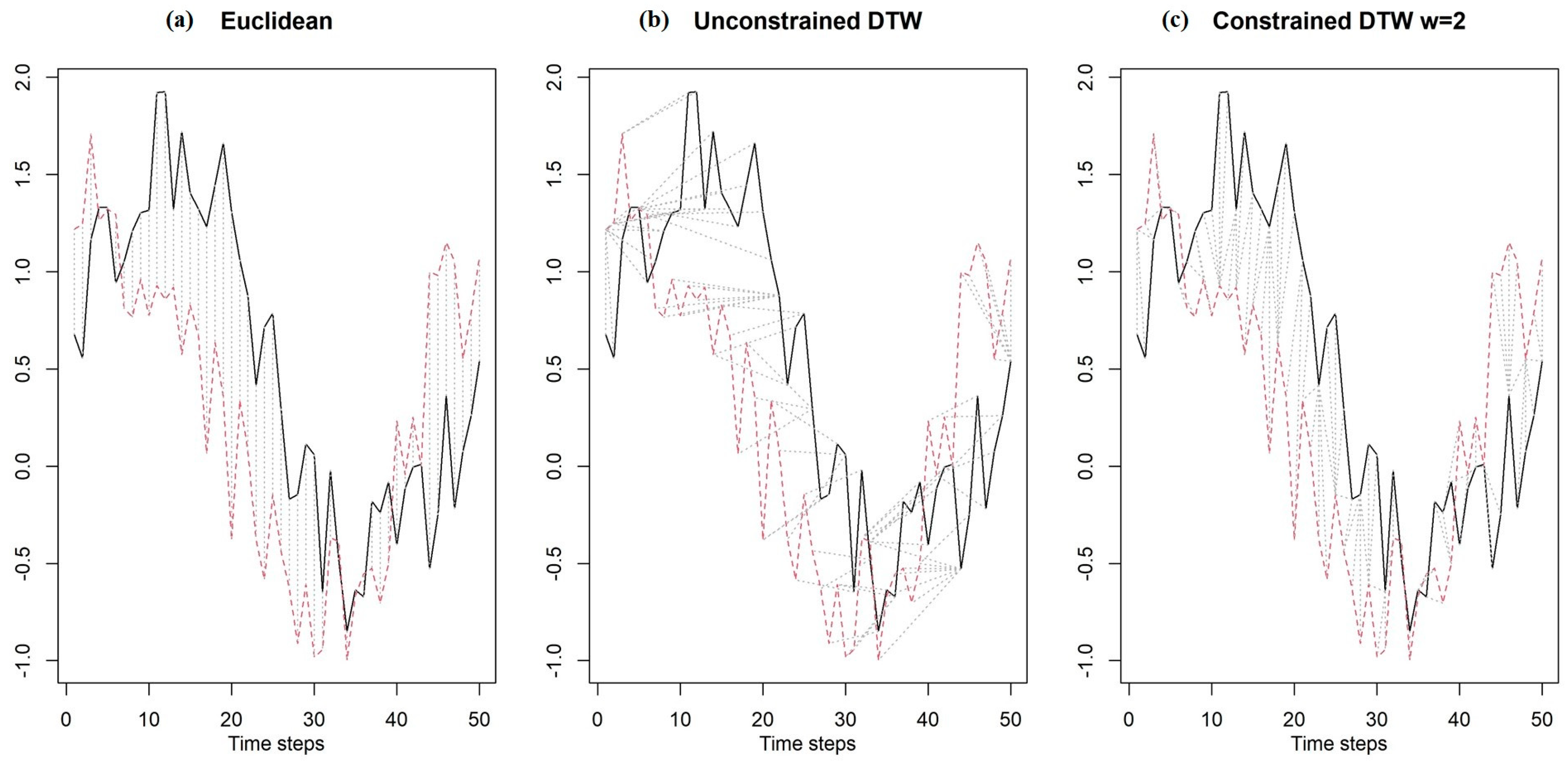
- Giorgino, T. Computing and Visualizing Dynamic Time Warping Alignments in R: The Dtw Package. J. Stat. Softw. 2009, 31, 1–24. [Google Scholar] [CrossRef]
- Haaf, E.; Barthel, R. An Inter-Comparison of Similarity-Based Methods for Organisation and Classification of Groundwater Hydrographs. J. Hydrol. 2018, 559, 222–237. [Google Scholar] [CrossRef]
- Chu, S.; Keogh, E.; Hart, D.; Pazzani, M. Iterative Deepening Dynamic Time Warping for Time Series. In Proceedings of the 2002 SIAM International Conference on Data Mining, Arlington, VA, USA, 11–13 April 2002; Society for Industrial and Applied Mathematics: Philadelphia, PA, USA, 2002; pp. 195–212. [Google Scholar] [CrossRef]
- Sakoe, H. Dynamic-Programming Approach to Continuous Speech Recognition. In 1971 Proceedings of the International Congress of Acoustics; Akademiai Kiado: Budapest, Hungary, 1971. [Google Scholar]
- Sakoe, H.; Chiba, S. Dynamic Programming Algorithm Optimization for Spoken Word Recognition. IEEE Trans. Acoust. 1978, 26, 43–49. [Google Scholar] [CrossRef]
- Dau, H.A.; Silva, D.F.; Petitjean, F.; Forestier, G.; Bagnall, A.; Mueen, A.; Keogh, E. Optimizing Dynamic Time Warping’s Window Width for Time Series Data Mining Applications. Data Min. Knowl. Discov. 2018, 32, 1074–1120. [Google Scholar] [CrossRef]
- Kryszczuk, K.; Hurley, P. Estimation of the Number of Clusters Using Multiple Clustering Validity Indices. In Multiple Classifier Systems. MCS 2010; Springer: Berlin/Heidelberg, Germany, 2010; Volume 3590, pp. 114–123. [Google Scholar]
- Arbelaitz, O.; Gurrutxaga, I.; Muguerza, J. An Extensive Comparative Study of Cluster Validity Indices. Pattern Recognit. 2013, 46, 243–256. [Google Scholar] [CrossRef]
- Rousseeuw, P.J. Silhouettes: A Graphical Aid to the Interpretation and Validation of Cluster Analysis. J. Comput. Appl. Math. 1987, 20, 53–65. [Google Scholar] [CrossRef]
- Kim, M.; Ramakrishna, R.S. New Indices for Cluster Validity Assessment. Pattern Recognit. Lett. 2005, 26, 2353–2363. [Google Scholar] [CrossRef]
- Saitta, S.; Raphael, B.; Smith, I.F.C. A Bounded Index for Cluster Validity. In Machine Learning and Data Mining in Pattern Recognition. MLDM 2007; Springer: Berlin/Heidelberg, Germany, 2007; pp. 174–187. [Google Scholar]
- Nijenhuis, I.; Schmidt, M.; Pellegatti, E.; Paramatti, E.; Richnow, H.H.; Gargini, A. A Stable Isotope Approach for Source Apportionment of Chlorinated Ethene Plumes at a Complex Multi-Contamination Events Urban Site. J. Contam. Hydrol. 2013, 153, 92–105. [Google Scholar] [CrossRef]
- Colyer, A.; Butler, A.; Peach, D.; Hughes, A. How Groundwater Time Series and Aquifer Property Data Explain Heterogeneity in the Permo-Triassic Sandstone Aquifers of the Eden Valley, Cumbria, UK. Hydrogeol. J. 2022, 30, 445–462. [Google Scholar] [CrossRef]
- Shen, S.; Chi, M. Clustering Student Sequential Trajectories Using Dynamic Time Warping. In Proceedings of the 10th International Conference on Educational Data Mining (EDM 2017), Wuhan, China, 25–28 June 2017; pp. 266–271. [Google Scholar]
- Lafare, A.E.A.; Peach, D.W.; Hughes, A.G. Use of Seasonal Trend Decomposition to Understand Groundwater Behaviour in the Permo-Triassic Sandstone Aquifer, Eden Valley, UK. Hydrogeol. J. 2016, 24, 141–158. [Google Scholar] [CrossRef]
- Zanotti, C.; Caschetto, M.; Bonomi, T.; Parini, M.; Cipriano, G.; Fumagalli, L.; Rotiroti, M. Linking Local Natural Background Levels in Groundwater to Their Generating Hydrogeochemical Processes in Quaternary Alluvial Aquifers. Sci. Total Environ. 2021, 805, 150259. [Google Scholar] [CrossRef]
- Stefania, G.A.; Zanotti, C.; Bonomi, T.; Fumagalli, L.; Rotiroti, M. Determination of Trigger Levels for Groundwater Quality in Landfills Located in Historically Human-Impacted Areas. Waste Manag. 2018, 75, 400–406. [Google Scholar] [CrossRef]
- Parrone, D.; Frollini, E.; Preziosi, E.; Ghergo, S. ENaBLe, an On-Line Tool to Evaluate Natural Background Levels in Groundwater Bodies. Water 2021, 13, 74. [Google Scholar] [CrossRef]
- Bouteraa, O.; Mebarki, A.; Bouaicha, F.; Nouaceur, Z.; Laignel, B. Groundwater Quality Assessment Using Multivariate Analysis, Geostatistical Modeling, and Water Quality Index (WQI): A Case of Study in the Boumerzoug-El Khroub Valley of Northeast Algeria. Acta Geochim. 2019, 38, 796–814. [Google Scholar] [CrossRef]
- Zolekar, R.B.; Todmal, R.S.; Bhagat, V.S.; Bhailume, S.A. Hydro—Chemical Characterization and Geospatial Analysis of Groundwater for Drinking and Agricultural Usage in Nashik District in Maharashtra, India. Environ. Dev. Sustain. 2021, 23, 4433–4452. [Google Scholar] [CrossRef]
- Egidio, E.; Mancini, S.; De Luca, D.A.; Lasagna, M. The Impact of Climate Change on Groundwater Temperature of the Piedmont Po Plain (NW Italy). Water 2022, 14, 2797. [Google Scholar] [CrossRef]
- Li, J.; Hassan, D.; Brewer, S.; Sitzenfrei, R. Is Clustering Time-Series Water Depth Useful? An Exploratory Study for Flooding Detection in Urban Drainage Systems. Water 2020, 12, 2433. [Google Scholar] [CrossRef]


| No. of Clusters | Sil↑ | SF↑ | CH↑ | DB↓ | DB*↓ | D↑ | COP↓ |
|---|---|---|---|---|---|---|---|
| 5 | 0.44 | 4.89 × 10⁻⁶ | 35.48 | 0.85 | 1.05 | 0.14 | 0.15 |
| 6 | 0.43 | 1.41 × 10⁻⁶ | 30.93 | 0.87 | 1.18 | 0.14 | 0.13 |
| 7 | 0.40 | 1.83 × 10⁻⁷ | 27.55 | 0.99 | 1.27 | 0.18 | 0.12 |
| 8 | 0.40 | 1.35 × 10⁻⁷ | 25.50 | 0.88 | 1.20 | 0.18 | 0.11 |
| 9 | 0.40 | 2.26 × 10⁻⁷ | 23.11 | 0.81 | 1.12 | 0.20 | 0.11 |
| 10 | 0.39 | 3.67 × 10⁻⁷ | 21.11 | 0.77 | 0.98 | 0.24 | 0.10 |
| No of Clusters | Sil↑ | SF↑ | CH↑ | DB↓ | DB*↓ | D↑ | COP↓ |
|---|---|---|---|---|---|---|---|
| 5 | 0.54 | 2.24 × 10⁻¹² | 20.52 | 0.39 | 0.45 | 0.13 | 0.06 |
| 6 | 0.38 | 3.63 × 10⁻¹³ | 20.97 | 0.44 | 0.60 | 0.09 | 0.04 |
| 7 | 0.38 | 9.33 × 10⁻¹⁵ | 22.05 | 0.46 | 0.55 | 0.16 | 0.04 |
| 8 | 0.34 | 2.22 × 10⁻¹⁶ | 24.66 | 0.58 | 0.84 | 0.11 | 0.03 |
| 9 | 0.37 | 0.00 | 23.51 | 0.60 | 0.74 | 0.15 | 0.03 |
| 10 | 0.37 | 2.22 × 10⁻¹⁶ | 21.93 | 0.52 | 0.64 | 0.16 | 0.02 |
Disclaimer/Publisher’s Note: The statements, opinions and data contained in all publications are solely those of the individual author(s) and contributor(s) and not of MDPI and/or the editor(s). MDPI and/or the editor(s) disclaim responsibility for any injury to people or property resulting from any ideas, methods, instructions or products referred to in the content. |
© 2022 by the authors. Licensee MDPI, Basel, Switzerland. This article is an open access article distributed under the terms and conditions of the Creative Commons Attribution (CC BY) license (https://creativecommons.org/licenses/by/4.0/).
Share and Cite
Zanotti, C.; Rotiroti, M.; Redaelli, A.; Caschetto, M.; Fumagalli, L.; Stano, C.; Sartirana, D.; Bonomi, T. Multivariate Time Series Clustering of Groundwater Quality Data to Develop Data-Driven Monitoring Strategies in a Historically Contaminated Urban Area. Water 2023, 15, 148. https://doi.org/10.3390/w15010148
Zanotti C, Rotiroti M, Redaelli A, Caschetto M, Fumagalli L, Stano C, Sartirana D, Bonomi T. Multivariate Time Series Clustering of Groundwater Quality Data to Develop Data-Driven Monitoring Strategies in a Historically Contaminated Urban Area. Water. 2023; 15(1):148. https://doi.org/10.3390/w15010148
Chicago/Turabian StyleZanotti, Chiara, Marco Rotiroti, Agnese Redaelli, Mariachiara Caschetto, Letizia Fumagalli, Camilla Stano, Davide Sartirana, and Tullia Bonomi. 2023. "Multivariate Time Series Clustering of Groundwater Quality Data to Develop Data-Driven Monitoring Strategies in a Historically Contaminated Urban Area" Water 15, no. 1: 148. https://doi.org/10.3390/w15010148
APA StyleZanotti, C., Rotiroti, M., Redaelli, A., Caschetto, M., Fumagalli, L., Stano, C., Sartirana, D., & Bonomi, T. (2023). Multivariate Time Series Clustering of Groundwater Quality Data to Develop Data-Driven Monitoring Strategies in a Historically Contaminated Urban Area. Water, 15(1), 148. https://doi.org/10.3390/w15010148