Development and Application of a Rainfall Temporal Disaggregation Method to Project Design Rainfalls

Abstract

A climate model is essential for hydrological designs considering climate change, but there are still limitations in employing raw temporal and spatial resolutions for small urban areas. To solve the temporal scale gap, a temporal disaggregation method of rainfall data was developed based on the Neyman–Scott Rectangular Pulse Model, a stochastic rainfall model, and future design rainfall was projected. The developed method showed better performance than the benchmark models. It produced promising results in estimating the rainfall quantiles for recurrence intervals of less than 20 years. Overall, the analysis results imply that extreme rainfall events may increase. Structural/nonstructural measures are urgently needed for irrigation and the embankment of new water resources.

1. Introduction

Over the last several decades, climate change has affected the hydrological cycle at different levels of observation at local and global scales [1]. In many regions, an increase in extreme precipitation frequency enhanced by climate change has been observed and it has ultimately affected water resources in terms of quantity and quality [2].

General Climate Models (GCMs) are essential for estimating precipitation for climate change scenarios. However, there are difficulties in applying them to small-scale watersheds (e.g., urban watersheds) due to their coarse spatiotemporal resolutions [3,4,5].

Coupled Model Intercomparison Project Phase 5 (CMIP5) provides a framework for coordinated climate change experimentation. The spatial resolution of models in the CMIP5 is about 100 km [6], and the temporal resolution of outputs ranges from 6-hourly data to monthly means. However, hydrological process analysis based on fine-resolution data at local scales is required to capture extreme changes in rainfall that may occur in catastrophic disasters. Recently, the Korea Meteorological Administration (KMA) began to provide 3 h temporal scale Regional Climate Model (RCM) outputs as a result of the Coordinated Regional Climate Downscaling EXperiment (CORDEX) program. However, as minute or hourly rainfall data are required to design hydraulic structures, downscaling techniques still need to obtain the desired temporal rainfall scale [7].

Downscaling techniques have been developed to bridge the scale gap between climate change scenarios and practical impact assessments [3,8]. Downscaling techniques are classified as a dynamic and statistical approach. Dynamical downscaling of RCMs into GCMs represents atmospheric physics with a fine grid size within a limited area of interest. Statistical downscaling establishes statistical links between large-scale weather and observed small-scale temperature [3]. However, dynamical downscaling has realistic constraints due to high computational costs, such as the enormous computation, storage space, and parameter estimation required, depending on the scale change. Therefore, statistical downscaling is computationally efficient while providing acceptable results [7]. In general, statistical downscaling means including both temporal and spatial downscaling, but spatial downscaling is not included since this study focused on temporal downscaling.

The rainfall disaggregation technique has recently been attracting attention as part of the statistical downscaling technique. Both disaggregation and downscaling techniques are similar in transferring information from a given scale to a smaller scale, but they are not identical [9]. Downscaling aims to produce data on a finer resolution that is statistically consistent with the data at a given resolution. On the other hand, disaggregation has the additional constraint that the disaggregated data must keep the statistical properties of the raw data regardless of its resolutions. Downscaling requires a complicated process to consider the surrounding observation stations, but disaggregation has the benefit of spatial correlation being fully considered at the resolution of a given set of data. Downscaling creates a new synthetic time series that statistically matches the target to be downscaled but cannot reproduce the time series of the target. However, there is a difference in that the rainfall disaggregation technique is statistically consistent and can almost completely produce the time series of the target.

Many studies on rainfall disaggregation have been conducted and stochastic rainfall models have mainly been used to disaggregate from daily to sub-daily levels. Debele et al. [10] investigated the suitability of deterministic and stochastic approaches to disaggregating daily meteorological data into hourly data in the Cedar Creek watershed, TX, USA. Abdellatif et al. [11] performed disaggregation of daily rainfall data based on the Bartlett–Lewis Rectangular Pulses (BLRP) model at three stations with different climate characteristics in the UK. Nourani and Farboudfam [12] evaluated the rainfall disaggregation performance of an AI-based model for daily and monthly rainfall, and Rafatnejad et al. [13] used weather variables and sub-daily characteristics affecting rainfall distribution to disaggregate daily rainfall into a 5 min time series.

Stochastic rainfall models based on Poisson cluster processes represent rainfall occurrence and amount as a single continuous process. They are attractive because they represent the observed temporal clustering nature of rainfall [14]. Two main versions of this model exist: the Bartlett–Lewis and the Neyman–Scott Rectangular Pulse model (BLRP and NSRPM), respectively, differing in terms of how pulses are distributed in relation to storm origin [15]. Both models perform well regarding observed statistical properties of rainfall series [16]. Although the literature on the differences between the NSRPM and the BLRPM is limited, it is known that the BLRPM is very sensitive to the sets of moment equations used in the parameter estimation as compared to the NSRPM [15,17]. The NSRPM, first applied in hydrology by Rodriguez-Iturbe et al. [18], has been extensively studied [16]. Entekhabi et al. [19] examined the NSRPM with a randomized parameter for the exponential distribution of rain cell durations. Cowperthwait [20] applied the NSRPM to a series of 10-year observations and examined the probability of dry periods. Cowpertwait [21] conducted a study to improve the reproduction of extreme values for sub-daily rainfall data. Afterward, parameter estimation, regionalization, and model improvement were implemented in several studies [22]. The temporal applicability of the NSRPM for a single site has been proven through several studies. Recently, studies on spatial applicability and rainfall simulation under weather types and climate change have also been conducted [23]. The NSRPM well reflects the cluster characteristics of Korean rainfall phenomena, which the original rectangular pulse model does not reflect, and many studies have been conducted [7].

Design rainfall is used in hydrological analysis, modeling, and urban stormwater drainage design [24]. A common practice is to perform a frequency analysis on the block (i.e., seasonal or annual) rainfall extreme using statistical distributions [15]. Rainfall extremes with finer temporal scales (e.g., 1 h or shorter) are necessary to design urban drainage systems because urban areas are generally characterized by rapid response [25]. In addition, it is essential to use rainfall data at finer temporal scales when using dynamic physical and biological models [10]. In this study, we develop a rainfall temporal disaggregation method to convert future rainfall data produced using a RCM into 1 h rainfall and project the behavior of future design rainfall for a short duration.

2. Materials and Methods

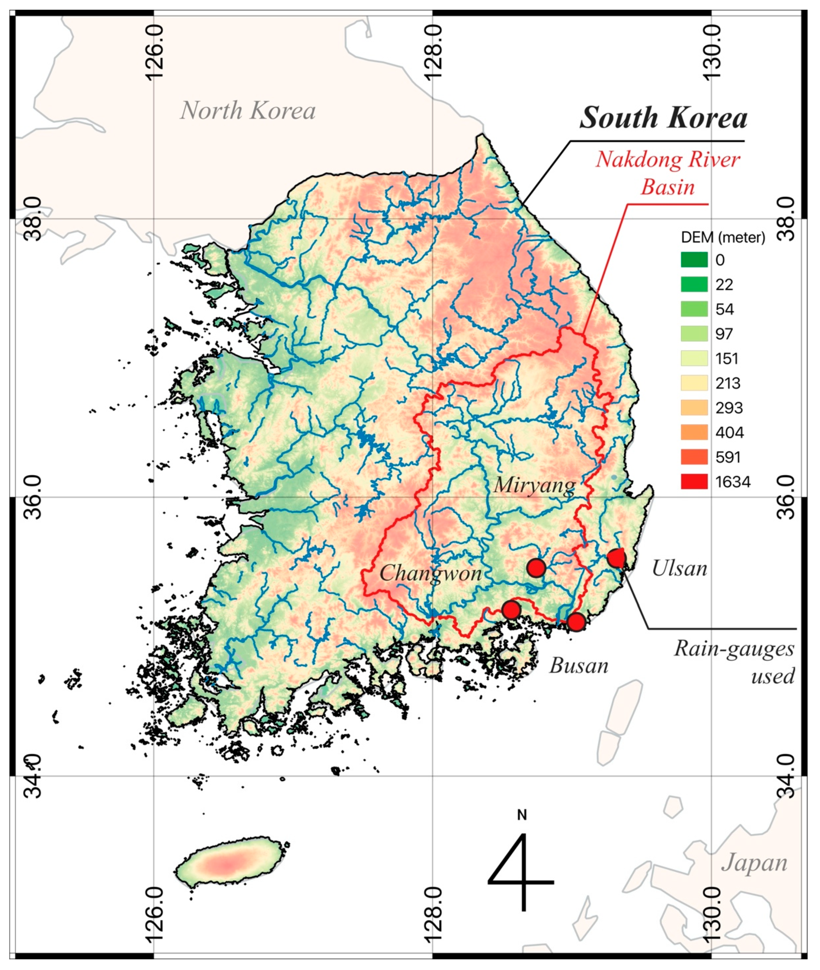
2.1. Study Area and Observation

The Nakdong River basin is located in the southeast of Korea between longitude 127°29′19″–129°18′00″ and latitude 34°59′41″–37°12′52″ (Figure 1). The area has four seasons with distinctive climatic features: Spring from March to May, Summer from June to August, Fall from September to November, and Winter from December to February [26]. The annual average temperature is 14.5 °C, the hottest month is August with a monthly average temperature of 25 °C, and the coldest month is January with a monthly average temperature of −7 °C. The annual precipitation range is roughly 1000 to 1850 mm (1270 mm on average). In general, there is a wet season from June to September (peaking in July), and 70% of annual precipitation occurs due to monsoons and typhoons [27]. The period from October to February is referred to as a dry season, and the period from November to February is referred to as a snow-dominated season [28].

The application basin has a drainage area of about 23,690 km²; it is 1/4 of the size of Korea [29]. The study area is the estuary basin located downstream of the Nakdong River, and the weather stations are Ulsan, Changwon, Busan, and Miryang. Weather observations included 30 years of observed hourly rainfall data from 1981 to 2010. However, in the case of Changwon, since observations started in 1985, only 25 years of observation data were used.

2.2. Climate Models

In this study, climate change scenarios for the Korean peninsula (KOR-11) were downscaled at 12.5 km horizontal resolution into the East Asian region, including the Korean peninsula, from the results of GCMs [30]. The KOR-11 provides a total of 16 dynamically downscaled future climate ensembles from a combination of four RCMs (MM5, WRF, RegCM, and RSM) and two GCMs, including HadGEM2-AO (Hadley Centre Global Environmental Model version 2 coupled with the Atmosphere–Ocean, hereafter HGEM) and MPI-ESM-LR (Max Planck Institute Earth System Model, low resolution, hereafter MPI) under RCP 4.5 and 8.5 climate change scenarios. The KOR-11 scenario provides high spatial resolution (12.5 km) simulations for the present period (also called the control period), 1981~2010, and for a future scenario, 2021~2050. The RCP 4.5 scenario was used in this study, focusing on July, which has the most frequent rainfall (Figure 2). Therefore, a total of 8 RCM Rainfall Data (RRD) were used, and the information on this is shown in

Table 1. The 8 RCMs used from the KOR-11.

Acronym	GCM	RCM	Period	Scale (Temporal, Spatial, Year)	Scenario
RRD 1	MPI_ESM_LR	MM5	Present 1981–2010	3 h, 12.5 km, 365 days	RCP 4.5
RRD 2	MPI_ESM_LR	WRF		3 h, 12.5 km, 365 days	RCP 4.5
RRD 3	MPI_ESM_LR	RegCM		3 h, 12.5 km, 365 days	RCP 4.5
RRD 4	MPI_ESM_LR	RSM		3 h, 12.5 km, 365 days	RCP 4.5
RRD 5	HadGEM2-AO	MM5	Future 2021–2050	3 h, 12.5 km, 365 days	RCP 4.5
RRD 6	HadGEM2-AO	WRF		3 h, 12.5 km, 365 days	RCP 4.5
RRD 7	HadGEM2-AO	RegCM		3 h, 12.5 km, 360 days	RCP 4.5
RRD 8	HadGEM2-AO	RSM		3 h, 12.5 km, 360 days	RCP 4.5

.

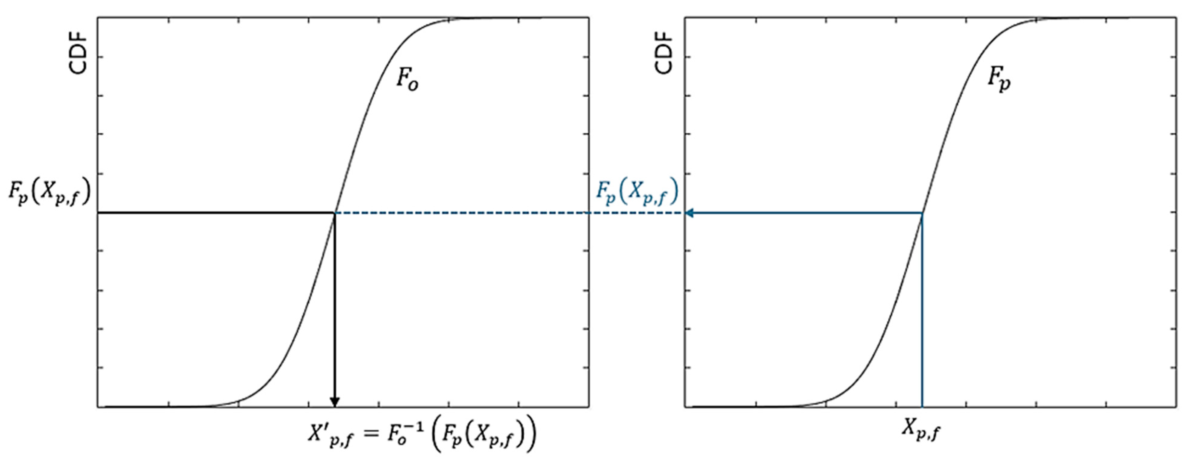
2.3. Bias Correction for Climate Model Data

To improve the simulated regional climate properties of the dynamical downscaling data, bias correction was implemented for the RCMs of the present and future periods [31]. Various bias correction methods have been developed, including Quantile Mapping (QM), Quantile Delta Mapping (QDM), and Detrended Quantile Mapping (DQM) [32]. This study employed QM, mainly used for bias correction, and the governing equations are as shown in Equations (1) and (2). A simple principle scheme of the bias correction method is shown in Figure 3.

The bias correction value, $X_p^{\prime }$, for the present period is calculated according to Equation (1).

$$X_p^{\prime }=F_o^{-1}\left(F_p\left(X_p\right)\right)$$

(1)

where $X_p$ is the original value of the present period of the RCM, $F_p$ is the Cumulative Distribution Function (CDF) of $X_p,$ and $F_o$ is the CDF of the observations.

The bias correction value, $X_f^{\prime },$ for the future period is calculated according to Equation (2).

$$X_f^{\prime }=F_o^{-1}\left(F_p\left(X_f\right)\right)$$

(2)

where $X_f$ is the original value of the future period of the RCM.

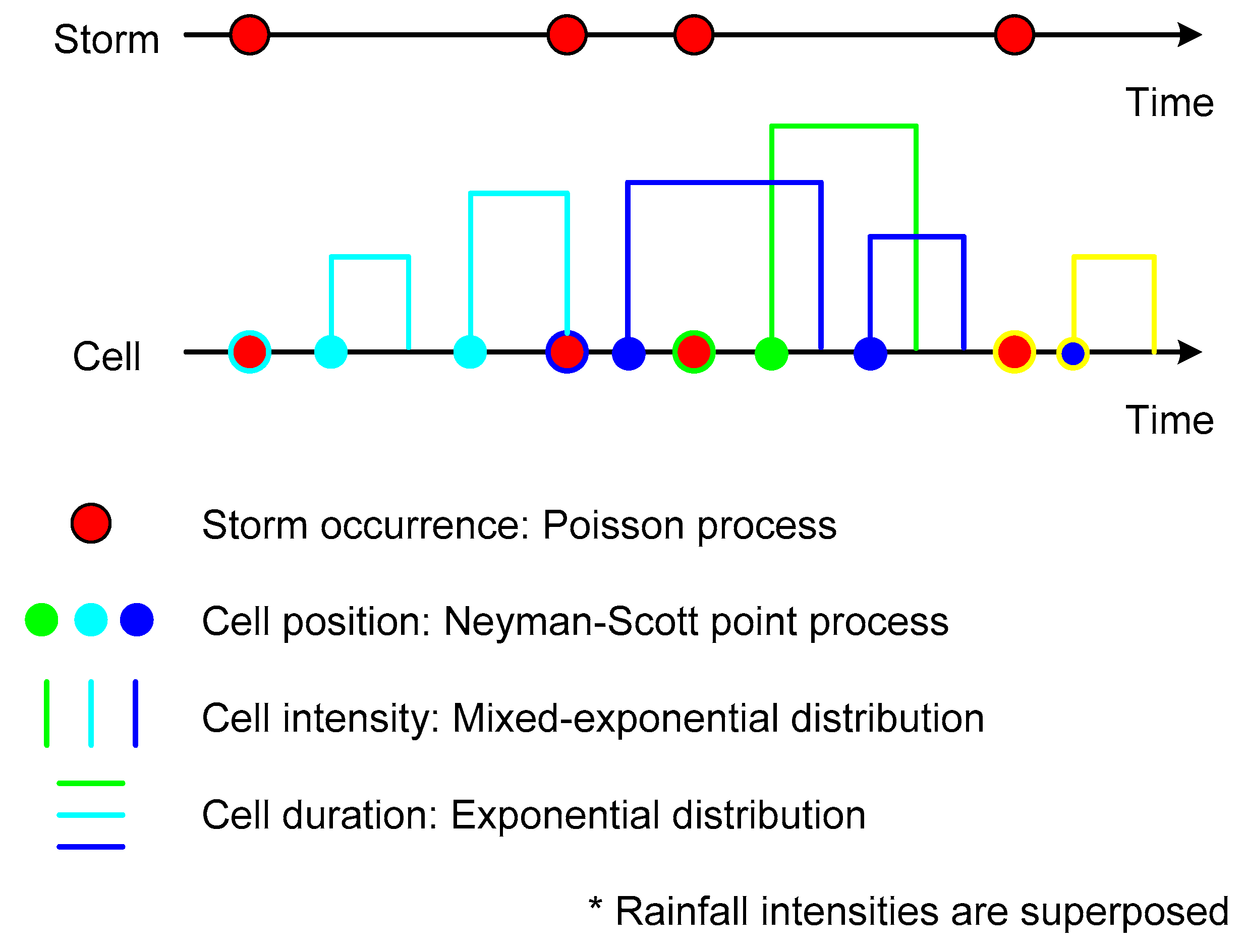
2.4. Neyman–Scott Rectangular Pulse Model (NSRPM)

The NSRPM (see Figure 4) is based on Poisson arrivals of storms and associated with each arrival is a cluster of rectangular pulses of random depth and duration, displaced randomly from the cluster origin. In the earliest model formulation, it is assumed that both the intensity and the duration of a pulse are independent and identically distributed, following an exponential distribution [15]. This study improved the NSRPM by assuming that the intensity of rainfall cells follows a three-variable mixed exponential distribution rather than a general applied exponential distribution. Previous studies have verified the suitability of the three-variate mixed index distribution for the Korean climate [33,34,35,36].

$$f\left(x\right)=\frac{\alpha }{\zeta }{e}^{-\frac{x}{\zeta }}+\frac{1-\alpha }{\theta }{e}^{-\frac{x}{\theta }}$$

(3)

where $x$ is the intensity of the rainfall cell and $\alpha$, $\zeta$, and $\theta$ are parameters of the three-variable mixed exponential distribution. The three-variable mixed exponential distribution can be seen as a weighted average of two parameters, $\zeta$ and $\theta$.

The first and second moments for the intensity of rainfall cells are as follows.

$$E\left[x\right]=\alpha \zeta +\left(1-\alpha \right)\theta$$

(4)

$$E\left[x^2\right]=2\alpha {\zeta }^2+2\left(1-\alpha \right){\theta }^2$$

(5)

Note that if $\alpha$ is specified as 1, it becomes a general exponential distribution and becomes the same model as the existing NSRPM.

According to Rodriguez-Iturbe [37], the mean and variance of rainfall time series $Y_i{}^{\left(h\right)}$ aggregated without overlap at h time intervals are as follows.

$$E\left[Y_i^h\right]=\frac{\lambda E\left[\nu \right]E\left[x\right]h}{\eta }$$

(6)

$$Var\left[Y_i^h\right]=\frac{\lambda }{{\eta }^3}\left(\eta h-1+e^{-\eta h}\right)\left\{2E\left[\nu \right]E\left[x^2\right]+\frac{\left(E^2\left[\nu \right]-1\right)E^2\left[x\right]{\beta }^2}{{\beta }^2-{\eta }^2}\right\}-\frac{\lambda \left(\beta h-1+e^{-\beta h}\right)\left(E^2\left[\nu \right]-1\right)E^2\left[x\right]}{\beta \left({\beta }^2-{\eta }^2\right)}$$

(7)

The probability that an arbitrary h time interval is dry ($Y_i{}^{\left(h\right)}=0$) was derived by Cowpertwait et al. [38].

$$\varphi \left(h\right)=Pr\left[Y_i^{\left(h\right)}\right]=e^{-\lambda h+\frac{\lambda (1-e^{1-E\left[\nu \right]+\left(E\left[\nu \right]-1\right)e^{-\beta h}}}{\beta E\left[\nu \right]-1}-\lambda {{\displaystyle \int }}_0^{\infty }\left[1-p_h\left(t\right)\right]dt}$$

(8)

$$p_h\left(t\right)=\left(e^{-\beta \left(t+h\right)}+1-\frac{\eta e^{-\beta h}-\beta e^{-\eta t}}{\eta -\beta }\right)e^{-\frac{\left(E\left[\nu \right]-1\right)\beta \left(e^{-\beta t}-e^{-\eta t}\right)}{\eta -\beta }-\left(E\left[\nu \right]-1\right)e^{-\beta t}+\left(E\left[\nu \right]-1\right)e^{-\beta \left(t+h\right)}}$$

(9)

The transition probability from wet to wet ${\varphi }_{ww}\left(h\right)$ and dry to dry ${\varphi }_{dd}\left(h\right)$ can be derived as follows.

$${\varphi }_{ww}\left(h\right)=\frac{1-2\varphi \left(h\right)+\varphi \left(2h\right)}{1-\varphi \left(h\right)}$$

(10)

$${\varphi }_{dd}\left(h\right)=\frac{\varphi \left(2h\right)}{\varphi \left(h\right)}$$

(11)

With the application of the three-variable mixed exponential distribution, the improved NSRPM has seven parameters (parameter $\lambda$ for the storm origin by Poisson process, parameter $E\left[\nu \right]$ for the number of rainfall cells, parameter $\beta$ for cell origin by an exponential distribution, parameter η for the cell duration by an exponential distribution, and parameters $\alpha$, $\zeta$, and $\theta$ for cell intensity by three-variable mixed exponential distribution) instead of the existing five.

The monthly parameter estimation process for the NSRPM can be summarized as follows.

(1)

Calculate the mean of 1 h rainfall, $E\left[Y_i^{1h}\right]$, the variance of 24 h rainfall, $Var\left[Y_i^{24h}\right]$, the transition probability from wet to wet, ${\varphi }_{ww}\left(24h\right)$ in 24 h (daily) rainfall, the transition probability from dry to dry, ${\varphi }_{dd}\left(24h\right)$ in 24 h (daily) rainfall, and the probability of zero depth, $\varphi \left(24h\right)$. $E\left[Y_i^{1h}\right]$ can be easily obtained by dividing the mean of input data by the temporal scale of input data. For example, if the input data is a 3 h scale rainfall, the 1 h mean rainfall is the input rainfall mean that is divided by 3.

(2)

Estimate the variance of 1, 3, 6, and 12 h rainfall, $Var\left[Y_i^{1h}\right]$, $Var\left[Y_i^{3h}\right]$, $Var\left[Y_i^{6h}\right]$, and $Var\left[Y_i^{12h}\right]$. It is known that it is desirable to construct a regression model with the variance of input data and the variance of the 1, 3, 6, and 12 h rainfall calculated from the observations for parameter estimation [21,23]. This assumes regional normality on a monthly scale and it is considered realistic to utilize empirical relationships rather than arbitrary distributions.

(3)

Ninety statistics, $E\left[Y_i^{1h}\right]$, $Var\left[Y_i^{1h}\right]$, $Var\left[Y_i^{3h}\right]$, $Var\left[Y_i^{6h}\right]$, $Var\left[Y_i^{12h}\right]$, ${\varphi }_{ww}\left(24h\right)$, ${\varphi }_{dd}\left(24h\right)$, and ${\varphi }_{dd}\left(24h\right),$ are used to estimate parameters to minimize the following objective function $S$ (Equation (12)), and genetic algorithms are used.

$$S={{\displaystyle \sum }}_{i=1}^9{w}_i{\left(\frac{f_i}{{\widehat{f}}_i}-1\right)}^2$$

(12)

where ${\widehat{f}}_i$ is the statistic $i$ obtained from the observations, $f_i$ is the statistic derived from the corresponding NSRPM results, and $w_i$ is the weight of statistic $i$. Since all statistics of the synthetic time series produced by the NSRPM are important in the rainfall disaggregation process, parameters are estimated by giving the same weight ($w_i$ = 1) for all statistics.

2.5. Rainfall Temporal Disaggregation Based on the NSRPM (RTD-NSRPM)

Once the parameter estimates of the NSRPM are completed, the user can produce synthetic hourly rainfall data that reproduces the statistical characteristics of the observed rainfall at the target point for the desired period. The rainfall disaggregation technique is based on the assumption that if a long-term synthetic time series is produced, it is similar to the statistics of observed rainfall.

A database was constructed by generating a synthetic time series for 10,000 years using the NSRPM. Rainfall disaggregation is implemented for each independent rainfall event, and the concept of Inter-Event Time Definition (IETD) was applied to identify individual rainfall events from long-term time series. A typical criterion is an IETD, the minimum dry period between two rainfall pulses [39].

The rainfall disaggregation process by separated rainfall events is as follows:

• Identification of the sequence of target rainfall events (wet = 0, dry = 1);
• Exploration of a synthetic time series with the same rainfall sequence; and
• Determination of the optimal time series that minimizes the following objective ($T$) among the explored synthetic time series.

$$T=\sqrt{\left[{{\displaystyle \sum }}_{i=1}^L{ln}^2\left(\frac{E_i+c}{D{B}_i+c}\right)\right]}$$

(13)

where $E_i$ is the time series for the target rainfall event, $D{B}_i$ is the synthetic time series with the same rainfall sequence, and $L$ is the rainfall duration. $c$ is a constant and 0.1 mm is applied. This prevents errors due to the zero value derived during the simulation.

In the case of rainfall events with very long wet days, it is practically challenging to obtain the same rainfall occurrence sequence from the database. Assuming that two or more rainfall events overlap, the disaggregation process was applied independently by separating them into arbitrary sub-events. The synthesized time series used once was excluded from the database to prevent the same time series from being used repeatedly.

However, even if an optimal time series that minimizes the objective function ($T$) is found, it is practically impossible to reproduce the sum of the target rainfall events completely. Accordingly, an adjustment procedure is performed. In this study, a proportional adjustment procedure in which conformity was confirmed through previous studies [36,40] was used, and the equation for this is as follows.

$$X_s={\overline{X}}_s\left(E/{{\displaystyle \sum }}_{j=1}^k{\overline{X}}_j\right) s=1,2,\dots ,k$$

(14)

Here, ${\overline{X}}_s$ is the initial value of the optimal time series that minimizes the objective function ($T$), $k$ is the temporal scale of the input data ($k$ = 3 in the case of 3 h rainfall), and $X_s$ is the final result of the applied rainfall disaggregation and proportional adjustment procedure and has a 1 h temporal resolution.

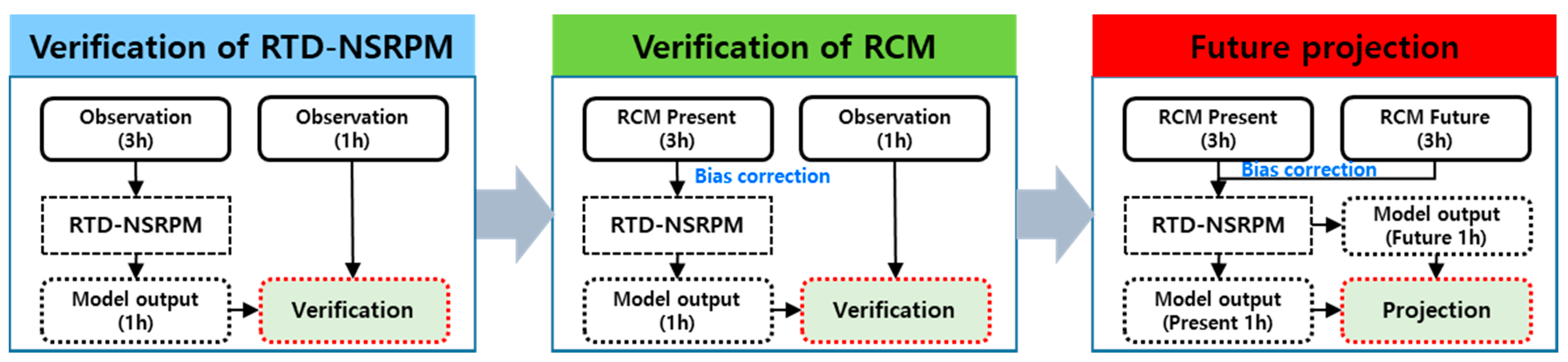
2.6. Evaluation Strategy

In this study, we develop the RTD-NSRPM method to convert future rainfall data produced using an RCM into 1 h rainfall. Based on this, we intend to project how the future design rainfall will change for a short duration. The research evaluation strategy is summarized in Figure 5, below, and the future short-duration design rainfall is projected through verification of the developed RTD-NSRPM and RCM data verification.

3. Results and Discussion

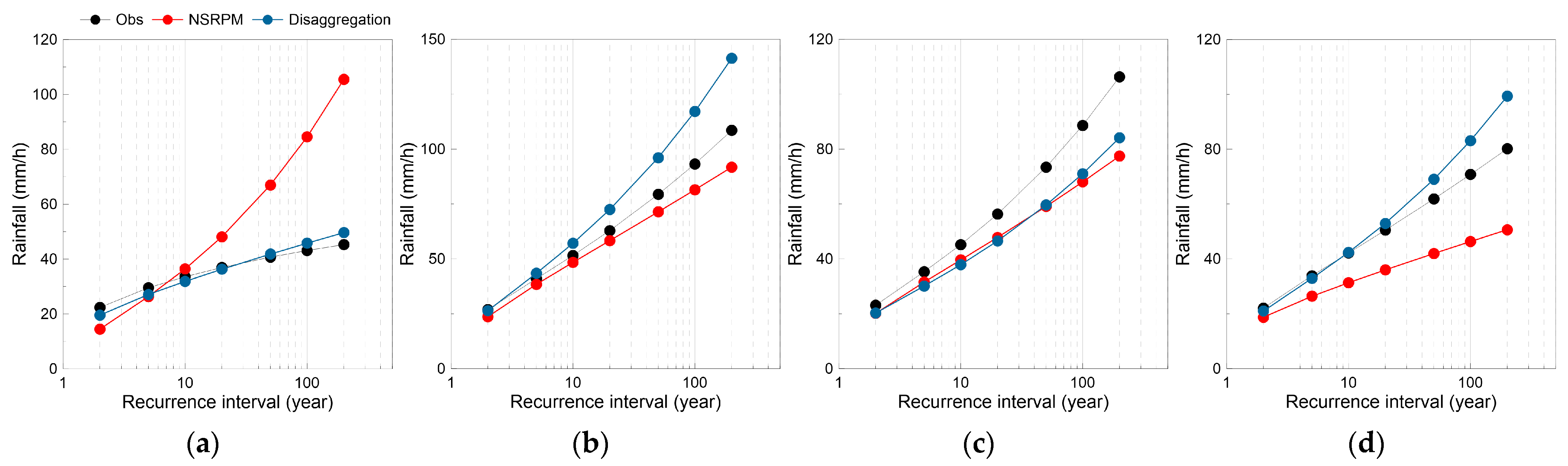
3.1. Verification of the RTD-NSRPM

The performance of the RTD-NSRPM method was verified using observation. Figure 6 shows the results of disaggregating the accumulated 3 h rainfall into 1 h rainfall. First, through the time series comparison results, it can be confirmed that the RTD-NSRPM results and the observed time series are quite similar (Figure 6a). The correlation coefficient between the two time series was significantly high, with an average of 0.75 at the four stations, and there was little difference between the stations (Figure 6b). Relative error results have shown that the RTD-NSRPM results tend to be underestimated compared to observations, with an average of −9% for four stations (Figure 6c). The root mean square error (RMSE) for the entire period was 2.0 mm with the average of four stations when zero values (no rainfall) were included and 4.0 mm when zero values were excluded. The average RMSE of the daily maximum 1 h rainfall was 4.7 mm, and the average RMSE for the monthly maximum 1 h rainfall was confirmed to be up to 9.5 mm. These results suggest that RTD-NSRPM estimates the temporal distribution of rainfall well, while uncertainty tends to increase as rainfall increases.

Figure 7 visualizes the scattering between the observation for each station and the RTD-NSRPM results. The daily maximum 1 h rainfall was used for comparison. As a result of a simple analysis of the variation at 5 mm intervals, the boundary threshold value between the high and low skill zones was 20 mm. It can be seen that the scattering degree varies depending on the size of the rainfall at all four stations. In particular, less than 20 mm of rainfall showed relatively dense scattering, whereas rainfall exceeding 20 mm showed severe dispersion. These results suggest that the RTD-NSRPM results for rainfall exceeding 20 mm may have limitations in terms of applicability.

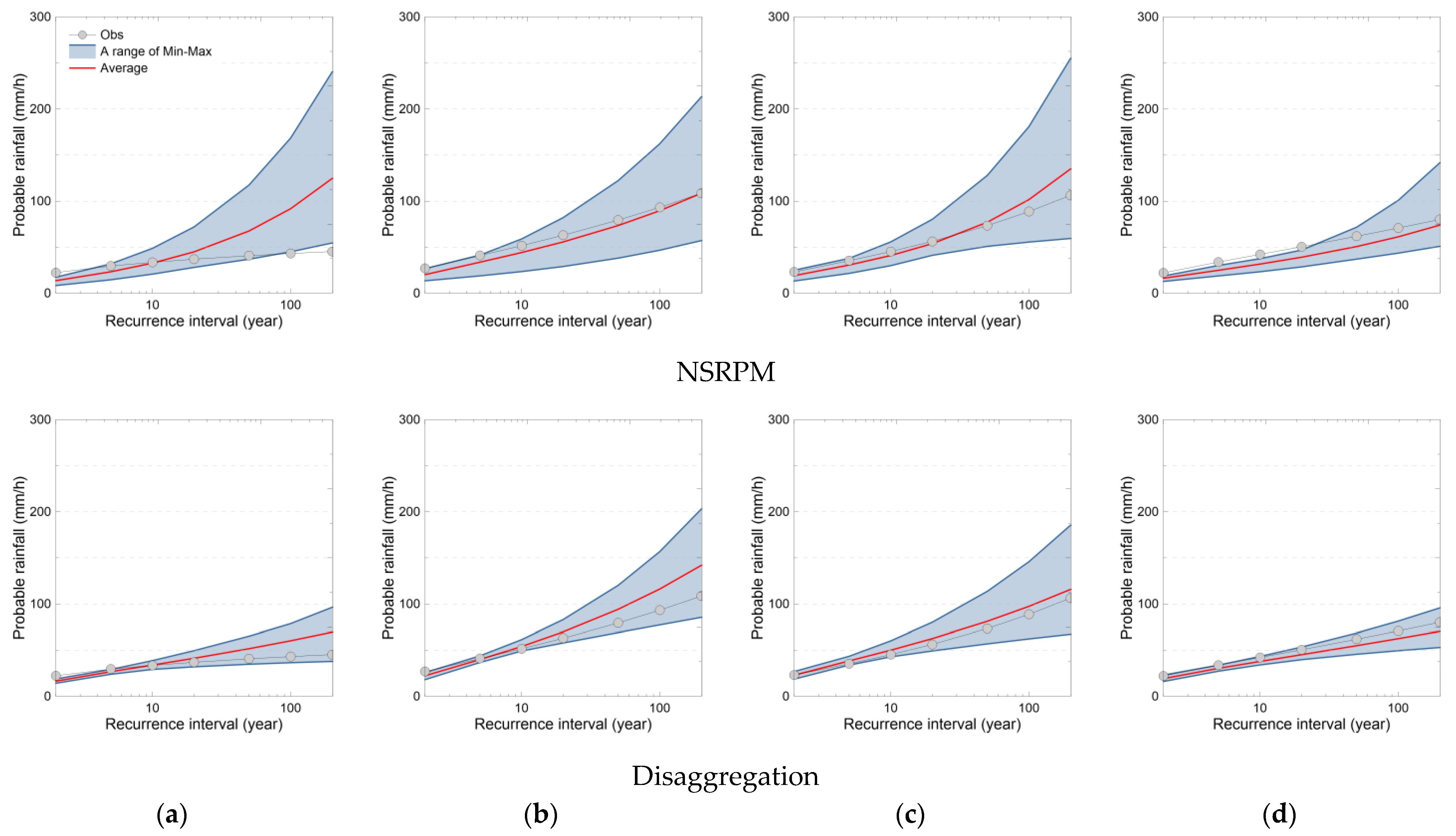
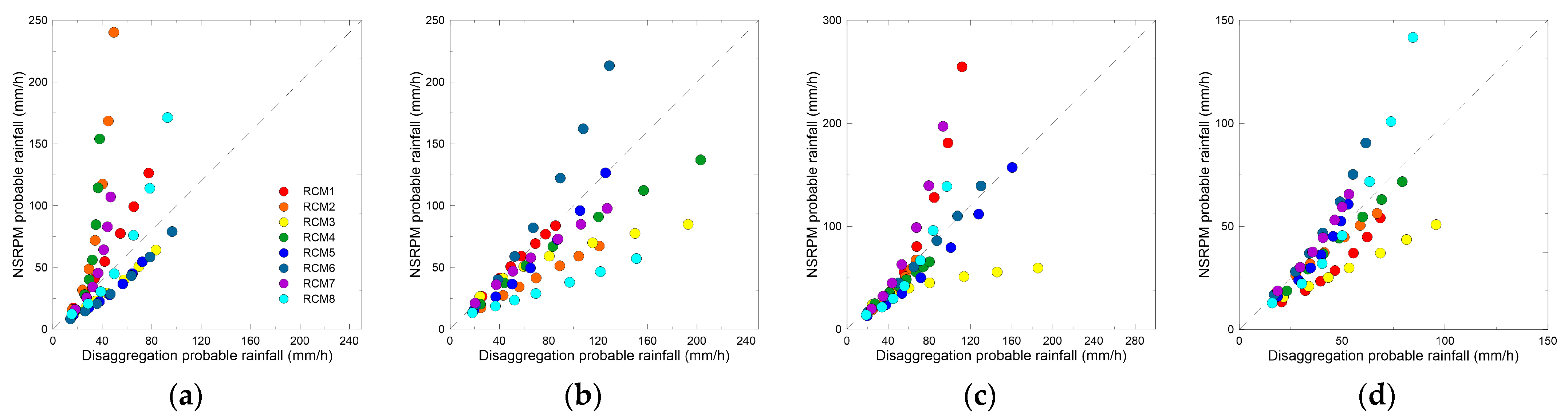
3.2. Comparison with the NSRPM

In this section, the rainfall quantiles estimated from the RTD-NSRPM and the NSRPM results are compared. Figure 8 shows the results of comparing the rainfall quantiles for each recurrence interval calculated from the downscaled rainfall by the two methods. The performance and suitability of the two methods were compared with the rainfall quantiles estimated by the observations. The review of the results found that the disaggregation (RTD-NSRPM) results were generally excellent in the recurrence interval of less than 20 years. However, it was found that both methods underestimated or overestimated the rainfall quantile exceeding the 20 year recurrence interval. In the case of Ulsan station, the NSRPM result tended to be significantly overestimated, and the Miryang station showed a significant tendency to underestimate.

Next, the results of the two methods for the RCM data were reviewed. Figure 9 shows the estimation results for the rainfall quantiles (for 2, 5, 10, 20, 50, 100, and 200 years) by the RCM for the present period. Eight RCM data were equally applied to both methods, and performance was verified by comparing the ranges of the rainfall quantile for each recurrence interval. The most significant difference in the rainfall quantile for each recurrence interval for the two methods is the maximum–minimum range of the eight RCM results. The NSRPM results showed reasonably high variability depending on the RCM, whereas the disaggregation method (RTD-NSRPM) showed a relatively stable range of rainfall quantiles. Disaggregation suggested a more reasonable range than the NSRPM at all stations.

As a singularity, the rainfall quantile estimated by the NSRPM at all stations tends to be underestimated in the short recurrence interval. For this reason, the average rainfall quantile of the NSRPM up to the 20-year recurrence interval was consistently underestimated compared to the observation. Disaggregation estimated the 1 h rainfall quantile that is relatively close to the observation until the recurrence interval of 20 years, and the rainfall quantile exceeding 20 years increased depending on the RCM. As confirmed in Figure 6 and Figure 7, it is considered that the downscaling error for relatively high rainfall acted as a source of uncertainty in the rainfall quantile estimation process.

The effect of the two methods on the rainfall quantile of each RCM was reviewed. Figure 10 is a scatter plot of the rainfall quantiles of the two methods. Figure 9 shows the rainfall quantile results for 7 (2, 5, 10, 20, 50, 100, and 200 years) recurrence intervals from 2 years to 200 years. The results were markedly different depending on the station. In particular, at the Ulsan station, the rainfall quantile of the NSRPM tended to be overestimated compared to the disaggregation method (RTD-NSRPM), while the opposite trend was confirmed at the Busan station. The results of the other two stations did not show any constant under- or overestimation trend. Considering that the uncertainty is included in the RCM itself, the uncertainty can be significantly amplified depending on the downscaling method.

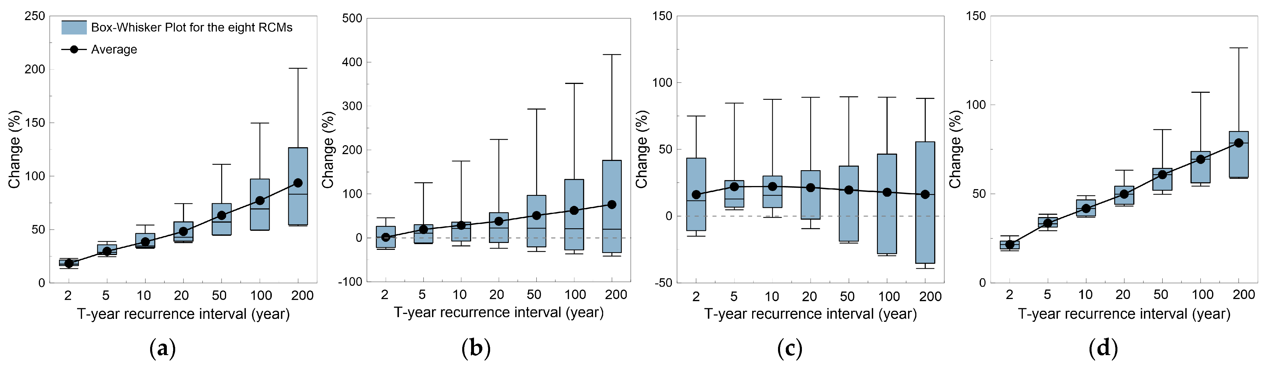
3.3. Projection of 1 h Maximum Rainfall

Figure 11 shows the projection results of the rainfall quantile increase/decrease rate (%) for each recurrence interval for the future period compared to the present period. The figure shows that the 1 h maximum rainfall for each recurrence interval is projected to increase in the future at all four stations. It was found that the 2-year recurrence interval increased to an average of 2–21% and the 200-year recurrence interval increased to an average of 16–93%. In the case of Ulsan and Miryang stations, the increase rate also tended to increase as the recurrence interval increased, so it is considered that the impact of climate change will be more significant than in other regions. Both Ulsan and Miryang stations are located within relatively complex mountainous areas. The mountainous effects are greater than those at the other two stations, so the increase in rainfall is expected to be more significant. On the other hand, the Busan and Changwon stations have more considerable variability in the rainfall quantile for each recurrence interval compared to the other two stations. Since it is located close to the coast, it seems that uncertainty in the RCM has played a somewhat significant role.

Considering that all eight RCM data applied were RCP 4.5 scenarios, in which efforts to reduce greenhouse gases have been partially effective, the region located downstream of the Nakdong River is likely to increase the hourly maximum rainfall/rainfall quantile. It was confirmed that the probability that the rainfall quantile for the recurrence interval less than 50 years in the future could be greater than the rainfall quantile for the recurrence interval of 200 years in the present period. In particular, in the case of the Ulsan station, the future rainfall quantile for the 20-year recurrence interval is greater than that in the present 200-year recurrence interval. Although this is a result that includes various uncertainties, it is thought that reorganization of the future urban watershed disaster prevention performance goals is necessary based on these results. In addition, since extreme rainfall may increase, it is considered that structural/nonstructural measures are urgently needed for irrigation and the embankment of new water resources.

4. Conclusions

In this study, the RTD-NSRPM method, a rainfall temporal disaggregation method, was developed to examine the future behavior of design rainfall that is variously applied in hydrological analysis and urban stormwater drainage design.

The developed method was verified with observed rainfall in July. Although it reproduces the temporal distribution of rainfall excellently, uncertainty tends to increase as the rainfall increases (e.g., the RSME of monthly maximum hourly rainfall was higher than daily maximum hourly rainfall). If daily maximum 1 h rainfall exceeds 20 mm, the accuracy of the RTD-NSRPM result may be slightly lower, so it is to be used with caution. In addition, a performance comparison of the NSRPM, which is the base model, and RTD-NSRPM methods was performed through the estimation of the rainfall quantile. The RTD-NSRPM method showed excellent results in estimating the rainfall quantile with a recurrence interval of less than 20 years. Although there were variations in the section with a recurrence interval of more than 20 years, the RTD-NSRPM method showed excellent results overall.

In the results of both methods for the July rainfall data of the present period of RCMs, the NSRPM showed significant variability depending on the RCM used. In contrast, the RTD-NSRPM showed a relatively stable range of rainfall quantiles, so it is expected that RTD-NSRPM can derive reliable results.

Lastly, the future projection results of the increase/decrease rates were reviewed through the ratio of the rainfall quantiles estimated from the RCM data for the present period and the future period. Ulsan and Miryang stations showed a clear tendency to increase the rate as the recurrence interval increased, but Busan and Changwon branches showed significant variations with respect to recurrence intervals. This is considered to reflect the characteristics of mountainous and coastal regions. It is expected that there is a high possibility that future rainfall in the study area will increase.

Although the proposed method is considered to help set future disaster prevention performance goals for urban watersheds, quantification research on uncertainty should be conducted considering that the results include various uncertainties. Furthermore, this study was conducted only for rainfall in July, which is the month with the most rainfall in Korea. Since it was assumed that the monthly rainfall distribution is stationary, research on other months or seasons also needs to be conducted.

References

1. Zhang, Y.; Li, H.; Reggiani, P. Climate Variability and Climate Change Impacts on Land Surface, Hydrological Processes and Water Management. Water 2019, 11, 1492. [Google Scholar] [CrossRef] [Green Version]
2. IPCC. 2014: Climate Change 2014: Synthesis Report. In Contribution of Working Groups I, II and III to the Fifth Assessment Report of the Intergovernmental Panel on Climate Change; Core Writing Team, Pachauri, R.K., Meyer, L.A., Eds.; IPCC: Geneva, Switzerland, 2014; p. 151. [Google Scholar]
3. Maraun, D.; Wetterhall, F.; Ireson, A.M.; Chandler, R.E.; Kendon, E.J.; Widmann, M.; Brienen, S.; Rust, H.W.; Sauter, T.; Themeßl, M.; et al. Precipitation downscaling under climate change: Recent developments to bridge the gap between dynamical models and the end user. Rev. Geophys. 2010, 48. [Google Scholar] [CrossRef]
4. Eden, J.M.; Widmann, M.; Maraun, D.; Vrac, M. Comparison of GCM- and RCM-simulated precipitation following stochastic postprocessing. J. Geophys. Res. Atmos. 2014, 119, 11040–11053. [Google Scholar] [CrossRef] [Green Version]
5. Tabari, H. Statistical Analysis and Stochastic Modelling of Hydrological Extremes. Water 2019, 11, 1681. [Google Scholar] [CrossRef] [Green Version]
6. Taylor, K.E.; Stouffer, R.J.; Meehl, G.A. An overview of CMIP5 and the experiment design. Bull. Am. Meteorol. Soc. 2012, 93, 485–498. [Google Scholar] [CrossRef] [Green Version]
7. Lee, J.; Jang, J.; Kim, S. Performance Evaluation of Rainfall Disaggregation according to Temporal Scale of Rainfall Data. J. Wetl. Res. 2018, 20, 345–352. [Google Scholar]
8. Jalota, S.K.; Vashisht, B.B.; Sharma, S.; Kaur, S. Chapter 2—Climate Change Projections. In Understanding Climate Change Impacts on Crop Productivity and Water Balance; Academic Press: Cambridge, MA, USA, 2018; pp. 55–86. [Google Scholar]
9. Lombardo, F.; Volpi, E.; Koutsoyiannis, D. Rainfall downscaling in time: Theoretical and empirical comparison between multifractal and Hurst-Kolmogorov discrete random cascades. Hydrol. Sci. J. 2012, 57, 1052–1066. [Google Scholar] [CrossRef] [Green Version]
10. Debele, B.; Srinivasan, R.; Parlange, J.Y. Accuracy evaluation of weather data generation and disaggregation methods at finer timescales. Adv. Water Res. 2007, 30, 1286–1300. [Google Scholar] [CrossRef]
11. Abdellatif, M.; Atherton, W.; Alkhaddar, R. Application of the Stochastic Model for Temporal Rainfall Disaggregation for Hydrological Studies in North Western England. J. Hydroinform. 2013, 15, 555–567. [Google Scholar] [CrossRef] [Green Version]
12. Nourani, V.; Farboudfam, N. Rainfall time series disaggregation in mountainous regions using hybrid wavelet-artificial intelligence methods. Environ. Res. 2019, 168, 306–318. [Google Scholar] [CrossRef]
13. Rafatnejad, A.; Tavakolifar, H.; Nazif, S. Evaluation of the climate change impact on the extreme rainfall amounts using modified method of fragments for sub-daily rainfall disaggregation. Int. J. Climatol. 2022, 42, 908–927. [Google Scholar] [CrossRef]
14. Burton, A.; Fowler, H.J.; Blenkinsop, S.; Kilsby, C.G. Downscaling transient climate change using a Neyman–Scott Rectangular Pulses stochastic rainfall model. J. Hydrol. 2010, 381, 18–32. [Google Scholar] [CrossRef]
15. Olsson, J.; Burlando, P. Reproduction of temporal scaling by a rectangular pulses rainfall model. Hydrol. Processes 2002, 16, 611–630. [Google Scholar] [CrossRef]
16. Cowpertwait, P.S.P.; Xie, G.; Isham, V.; Onof, C.; Walsh, D.C.I. A fine-scale point process model of rainfall with dependent pulse depths within cells. Hydrol. Sci. J. 2011, 56, 1110–1117. [Google Scholar] [CrossRef] [Green Version]
17. Velghe, T.; Troch, P.A.; De Troch, F.P.; Van de Velde, J. Evaluation of cluster-based rectangular pulses point process models for rainfall. Water Resour. Res. 1994, 30, 2847–2857. [Google Scholar] [CrossRef]
18. Rodriguez-Iturbe, I.; De Power, B.F.; Valdes, J.B. Rectangular pulses point process models for rainfall: Analysis of empirical data. J. Geophys. Res. Atmos. 1987, 92, 9645–9656. [Google Scholar] [CrossRef]
19. Entekhabi, D.; Rodriguez-Iturbe, I.; Eagleson, P.S. Probabilistic representation of the temporal rainfall process by a modified Neyman-Scott rectangular pulses model: Parameter estimation and validation. Water Resour. Res. 1989, 25, 295–302. [Google Scholar] [CrossRef] [Green Version]
20. Cowpertwait, P.S. Further developments of the Neyman-Scott clustered point process for modeling rainfall. Water Resour. Res. 1991, 27, 1431–1438. [Google Scholar] [CrossRef]
21. Cowpertwait, P.S. A generalized point process model for rainfall. Proc. R. Soc. London Ser. A Math. Phys. Sci. 1994, 447, 23–37. [Google Scholar]
22. Onof, C.; Chandler, R.E.; Kakou, A.; Northrop, P.; Wheater, H.S.; Isham, V. Rainfall modelling using Poisson-cluster processes: A review of developments. Stoch. Environ. Res. Risk Assess. 2000, 14, 384–411. [Google Scholar] [CrossRef]
23. Burton, A.; Kilsby, C.G.; Fowler, H.J.; Cowpertwait, P.S.P.; O’connell, P.E. RainSim: A spatial–temporal stochastic rainfall modelling system. Environ. Model. Softw. 2008, 23, 1356–1369. [Google Scholar] [CrossRef]
24. Haddad, K.; Rahman, A. Derivation of short-duration design rainfalls using daily rainfall statistics. Nat. Hazards 2014, 74, 1391–1401. [Google Scholar] [CrossRef]
25. Nguyen, V.T.V.; Nguyen, T.D.; Wang, H. Regional estimation of short duration rainfall extremes. Water Sci. Technol. 1998, 37, 15–19. [Google Scholar] [CrossRef]
26. Kim, J.; Park, M.; Joo, J. Comparison of characteristics and spatial distribution tendency of daily precipitation based on the regional climate models for the Korean Peninsula. J. Korean Soc. Hazard Mitig. 2015, 15, 59–70. [Google Scholar] [CrossRef] [Green Version]
27. Kim, J.; Joo, J. Characteristics of daily precipitation data based on the detailed climate change ensemble scenario depending on the regional climate models and the calibration. J. Korean Soc. Hazard Mitig. 2015, 15, 261–272. [Google Scholar] [CrossRef] [Green Version]
28. Joo, J.; Kim, S.; Park, M.; Kim, J. Evaluation and calibration method proposal of RCP daily precipitation data. J. Korean Soc. Hazard Mitig. 2015, 15, 79–91. [Google Scholar] [CrossRef] [Green Version]
29. Lee, J.; Kim, U.; Kim, L.H.; Kim, E.S.; Kim, S. Management of organic matter in watersheds with insufficient observation data: The Nakdong River basin. Desalinat. Water Treat. 2019, 152, 44. [Google Scholar] [CrossRef] [Green Version]
30. Kim, K.; Choi, J.; Lee, O.; Cha, D.H.; Kim, S. Uncertainty quantification of future design rainfall depths in Korea. Atmosphere 2020, 11, 22. [Google Scholar] [CrossRef] [Green Version]
31. Boé, J.; Terray, L.; Habets, F.; Martin, E. Statistical and dynamical downscaling of the Seine basin climate for hydro-meteorological studies. Int. J. Climatol. J. R. Meteorol. Soc. 2007, 27, 1643–1655. [Google Scholar] [CrossRef]
32. Cannon, A.J.; Sobie, S.R.; Murdock, T.Q. Bias correction of GCM precipitation by quantile mapping: How well do methods preserve changes in quantiles and extremes? J. Clim. 2015, 28, 6938–6959. [Google Scholar] [CrossRef]
33. Kim, S.; Han, S. Urban Stormwater Capture Curve Using Three-Parameter Mixed Exponential Probability Density Function and NRCS Runoff Curve Number Method. Water Environ. Res. 2010, 82, 43–50. [Google Scholar] [PubMed]
34. Choi, C.H.; Cho, S.; Park, M.J.; Kim, S. Overflow risk analysis for designing a nonpoint sources control detention. Water Environ. Res. 2012, 84, 434–440. [Google Scholar] [CrossRef] [PubMed]
35. Lee, O.; Choi, J.; Jang, S.; Kim, S. Application of Stochastic Point Rainfall Model for Temporal Downscaling of Daily Precipitation Data. J. Korean Soc. Hazard Mitig. 2017, 17, 323–337. [Google Scholar] [CrossRef]
36. Lee, J.; Kim, S. Temporal Disaggregation of Daily Rainfall data using Stochastic Point Rainfall Model. J. Korean Soc. Hazard Mitig. 2018, 18, 493–503. [Google Scholar] [CrossRef] [Green Version]
37. Rodríguez-Iturbe, I. Scale of fluctuation of rainfall models. Water Resour. Res. 1986, 22, 15S–37S. [Google Scholar] [CrossRef]
38. Cowpertwait, P.S.P.; O’Connel, P.E.; Metcalfe, A.V.; Mawdsley, J.A. Stochastic point process modeling of rainfall: 1. Single-site fitting and validation. J. Hydrol. 1996, 175, 17–46. [Google Scholar] [CrossRef]
39. Joo, J.; Lee, J.; Kim, J.H.; Jun, H.; Jo, D. Inter-event time definition setting procedure for urban drainage systems. Water 2014, 6, 45–58. [Google Scholar] [CrossRef] [Green Version]
40. Koutsoyiannis, D.; Onof, C. Rainfall disaggregation using adjusting procedures on a Poisson cluster model. J. Hydrol. 2001, 246, 109–122. [Google Scholar] [CrossRef]
Figure 1. Nakdong estuary basin and weather stations.
Water 14 01401 g001
Figure 2. Monthly rainfall of 30-year average (1981–2010) in the study area.
Water 14 01401 g002
Figure 3. Simple principle scheme of the bias correction technique.
Water 14 01401 g003
Figure 4. A Schematic depiction of the NSRPM.
Water 14 01401 g004
Figure 5. A schematic diagram of the evaluation strategy.
Water 14 01401 g005
Figure 6. Verification results of the disaggregation method against 1 h rainfall observed data. (a) Comparison of time series data, (b) correlation coefficient, (c) relative error (%) of daily maximum 1 h rainfall, representing underestimation with a negative value and overestimation with a positive value, and (d) RMSE (mm). In the RMSE result, ‘All’ indicates the results for the entire application period (including with or without zero values), and ‘Daily’ shows the results for the daily maximum 1 h rainfall.
Water 14 01401 g006
Figure 7. Scatter plots of daily maximum 1 h rainfalls from the observed data (X-axis) and the disaggregation method (Y-axis). (ad) show Ulsan, Busan, Changwon, and Miryang in order. The red dotted line is a threshold of 20 mm rainfall. The solid black line is a regression line in Y = a·X formula.
Water 14 01401 g007
Figure 8. Comparison of T-year recurrence interval (2~200 years) rainfalls from the observed (black), NSRPM (Red), and disaggregation (Blue) rainfalls. (a) Ulsan, (b) Busan, (c) Changwon, and (d) Miryang.
Water 14 01401 g008
Figure 9. Comparison of T-year rainfall quantile based on the downscaled 1 h rainfall from the NSRPM and RTD-NSRPM methods for the present period. (a) Ulsan, (b) Busan, (c) Changwon, and (d) Miryang.
Water 14 01401 g009
Figure 10. Scatter plots of the rainfall quantile based on the downscaled 1 h rainfalls from the NSRPM and disaggregation methods for the present period. (a) Ulsan, (b) Busan, (c) Changwon, (d) and Miryang.
Water 14 01401 g010
Figure 11. Change rate (%) of the future (2021–2050) T-year rainfall quantile based on the RTD-NSRPM method. (a) Ulsan, (b) Busan, (c) Changwon, and (d) Miryang.
Water 14 01401 g011