Article

Insights into Flood Wave Propagation in Natural Streams as Captured with Acoustic Profilers at an Index-Velocity Gaging Station

1
IIHR-Hydroscience & Engineering, The University of Iowa, Iowa City, IA 52242, USA
2
Civil & Environmental Engineering, Dankook University, 16890 Yongin, Gyeonggi, Korea
*
Authors to whom correspondence should be addressed.
Water 2022, 14(9), 1380; https://doi.org/10.3390/w14091380
Submission received: 16 February 2022 / Revised: 11 April 2022 / Accepted: 17 April 2022 / Published: 24 April 2022

Abstract

:
Recent advances in instruments are transforming our capabilities to better understand, monitor, and model river systems. The present paper illustrates such capabilities by providing new insights into unsteady flows captured with a Horizontal Acoustic Current Profiler (HADCP) integrated at an operational index-velocity gaging station. The illustrations demonstrate that the high-resolution stage and velocity measurements directly acquired during flood wave propagation reveal the intricate interplay among flow variables that are essential for better supporting judicious decision making for river management, flooding, sediment transport, and stream ecology. The paper confirms that the index-velocity method better captures the unsteady flow dynamics in comparison with the stage-discharge monitoring approach. At a time when the intensity and frequency of floods is continuously increasing, a better understanding of the critical features of flood waves during extreme events and the possibility of capturing more accurately their dynamics in real time is of special socio-economic significance.

1. Introduction

Monitoring and predicting streamflows are at the core of the decision making for critical areas of the socio-economic continuum (from water management, energy development, infrastructure design, and recreational uses to forecasting of floods, water quality, and ecosystem viability). While most often collected by specialized agencies, the streamflow data are also used as benchmarks for advancing the understanding of watershed dynamics and underpinning scientific studies on aquatic habitat and climate trends. The measurement protocols used for collecting streamflow data stem from century-long incremental developments [1]. Most of these developments have considered river flows as quasi-stationary processes fluctuating within an unchanging envelope of variability [2]. This view has given rise to empirical or semi-empirical relationships for streamflow estimation complemented by statistical analyses applied to long historical collected during steady and unsteady flows. While this estimation approach might be acceptable for reporting daily discharges for various uses, it is not satisfactory for practical and scientific investigations where the data are desired at sub-daily sampling rates [3]. Such an example is the propagation of flood waves generated by storms that are driven by gradual, time-varying flows with significant hourly variations.
During the gradually varied changes, the flow is affected by both unsteadiness and non-uniformity [4,5]. Depending on the slope of the stream bed and the magnitude and duration of the storm runoff entering the stream, the flood wave can take various forms, i.e., kinematic, diffusion, or full dynamic [6]. The dependencies among the flow variables during the wave propagation are distinct for the rising and falling stages and different from the steady flow relationships. This peculiar dependency is called hysteresis, which is a generic term denoting that the state of a system at any time depends on its past state (i.e., rising or falling). The hysteretic behavior is materialized as “loops” in the relationships between pairs of flow variables [7] and a separation of the flow hydrographs as discussed in [8]. Streams in low- and mild-sloped streams tend to produce considerable hysteresis for large flow changes occurring over short durations [9,10]. Streams on steep slopes display small hysteretic effects [11].
The most reliable method to truthfully capture hysteresis is the direct measurement of the discharge along with other relevant flow variables over the whole duration of the wave propagation. However, direct measurements require personnel deployment for extended time, especially in medium and large-size rivers. Moreover, stream measurements during extreme flows are challenging because of the difficulty accessing the sites and other safety concerns [12,13]. Consequently, streamflow monitoring in natural streams is typically made with indirect methods relying on pre-constructed rating curves used in conjunction with continuously measured variables that can be measured unattended. The most popular methods for real-time monitoring are the stage-discharge and index-velocity methods, which are labeled herein as HQRC and IVRC, respectively. These methods are well documented in multiple sources [12,14,15,16,17] therefore, only their salient features will be presented herein. The United States Geological Survey (USGS) publishes real-time discharge data for more than 10,000 sites across the US, with most of them relying upon HQRC method [3]. There are about 500 IVRC-based stations in the US, and their number continues to increase. At about 4000 of the total number of gages, streamflow forecasting is made via hydrologic modeling.
The HQRC streamflow estimation method was developed first, and it is still widely used to date for monitoring steady and unsteady flows. The simple HQRC is governed by equations that are strictly valid for steady flows whereby the energy and river-bed slopes are equal. However, during flood wave propagation, the energy slope is not equal to the bed slope being influenced by additional parameters; therefore, the estimates provided by steady HQRC are not capturing the actual flows [7]. Deviations as large as 9.8%, 15%, and 34% in discharges for the same stage were reported between actual and estimated HQRC flows in large rivers [15,18,19]. Differences up to 40% were found between Acoustic Doppler Current Profiler (ADCP) directly measured discharges and HQRC estimates in a medium-size, lowland river during unsteady flows [20]. A recent USGS evaluation conducted at 5420 HQRC stations found that 67% of them are moderately or strongly affected by hysteresis [3]. Corrections are applied to the simple HQRC for gages located in large rivers exposed to hysteresis [21]. For gages located on medium and small rivers, the correction for hysteresis is not applied, as there is a perception that its impact is small and cannot be discerned from instrument uncertainty [3].
The IVRC method is a better alternative to HQRC when monitoring unsteady flows because it measures directly the index velocity in addition to the stage [8]. This method has been increasingly implemented after the adoption of acoustic-Doppler velocimetry in the late 1990s [22], especially for locations where hysteresis and/or backwater might occur [16]. While the IVRC method can capture hysteresis in real time [23], the hydrometric community continues to test, evaluate, and improve IVRC capabilities (e.g., [24,25]). Due to the high cost of these evaluations and the methods’ shorter life span compared with the century-old HQRC, the IVRC method has been less investigated so far.
The motivation for this paper is triggered by the fact that while both HQRC and IVRC have been continuously improved through the incorporation of new measurement technologies (acoustic, radar, image velocimetry), the principles and assumptions associated with the conventional monitoring protocols have not been revised to take full advantage of the superior capabilities of the new instruments. This paper addresses this gap by evaluating how the IVRC method equipped with new measurement technology compares with HQRC (used as reference herein) and revealing new features of the mechanisms in unsteady flows. Exploration of these features is rarely illustrated with data acquired in situ. The data-driven exploration on flood wave propagation presented in this paper is intentionally kept in a simple form to substantiate the hysteresis phenomenology and dependencies rather than cluttering the narration with analytical and statistical analysis.
The paper is organized as follows. First, it reviews the principles and practice of the conventional HQRC and IVRC along with their advantages and limitations. Aspects of flow dependencies during the propagation of flood waves are then illustrated with data acquired at an operational IVRC-based gaging station served by an emerging instrument: the Horizontal Acoustic Doppler Current Profiler (HADCP). Subtle features of the hysteretic behavior are then highlighted to illustrate the potential of the IVRC method to document flow features that might broaden the use of data for practical and scientific purposes. Finally, the paper suggests research for further evaluation of the hysteresis impact on monitoring methods and for developing protocols that can reduce their uncertainty.

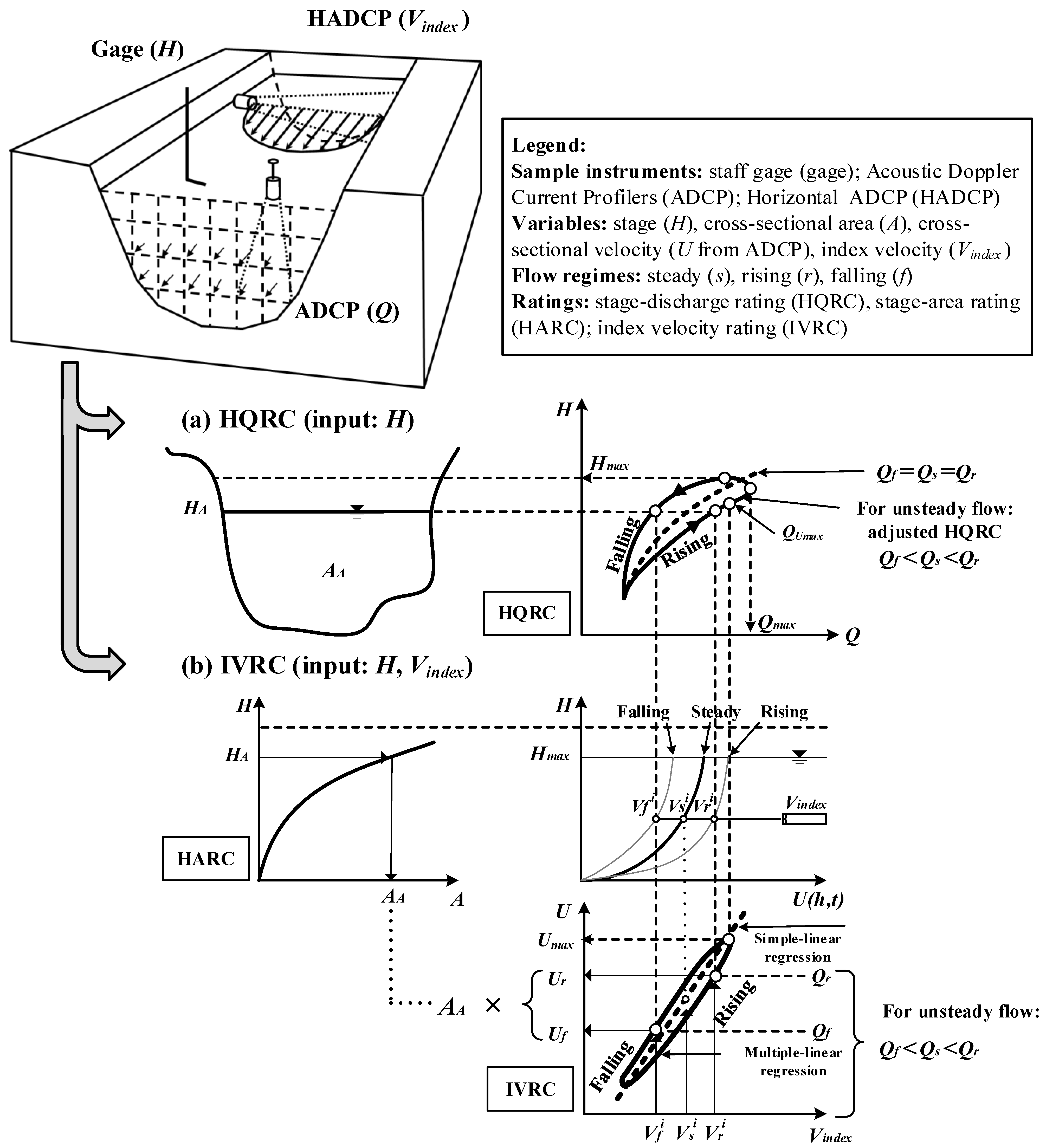
2. Principles and Practice of Conventional Monitoring Methods

Conventional monitoring methods are based on semi-empirical relationships that relate in situ discharge measurements with flow variables directly acquired at monitoring site. These relationships (a.k.a., ratings) are valid only for the site where they were constructed. Rating construction assumes that the stream gauge sites are closely following the best practices for gage site selection (e.g., Rantz et al. [14]). Among these guidelines, critical ones include free of obstructions or bed irregularities in the channel reach enclosing the gaging station, quasi-uniform geometry in the streamwise direction, and preservation of the cross-sectional flow distribution for the whole range of flows at the station.
The independent flow variables used in conjunction with the ratings are those that can be continuously measured without operator assistance (i.e., stage and, more recently, velocity distributions along lines or surfaces into the flow). The guidelines for rating construction typically assumes a one-to-one relationship among flow variables without specifically distinguishing between the rising and falling phases of the flood wave. The final ratings are established only after an extended dataset of calibration measurements are acquired, processed, and checked for consistency with statistical tools. In many situations, the overall quality of the final rating is highly contingent on the operator’s skills and his/her specific knowledge of the measurement site.
The steady HQRCs are obtained through graphical constructions guided by analytical relationships, i.e., flow over weirs at low flows, Manning’s equation at higher stages up to the bankful stage, and by other approaches for extreme flows [7,14]. This rating misses the hysteretic signature altogether, as the Q = f (H) relationship is the same for the rising and falling limbs of the hydrograph (see dotted line in Figure 1a). The steady HQRC method leads to a maximum value for discharge hydrograph, Qmax, when Hmax is attained. Notably, the discharge corresponding to the maximum cross-section velocity, QUmax, does not coincide with the position of the actual Qmax on the loop. Corrections [21,26,27] can be applied in post-processing to the steady HQRC estimated discharge to uncover the hysteretic loop associated with the passing of flood wave through a gauging site (continuous line in Figure 1a). Given their costs, these corrections are only applied at selected gages, especially for those located in flood-prone areas along large rivers [3].
The IVRC method has become increasingly popular after the adoption of HADCPs for river measurements [16]. The latter authors specify that the method has been developed for sites where “more than one specific discharge can be measured for a specific stage”, which are situations specific for flood wave propagation in lowland streams [8]. The main steps involved in the construction and monitoring with the IVRC method are shown in Figure 1b. First, a stage-area (HARC) is constructed to relate the range of stages measured at the station with the corresponding areas for the wetted cross-section (continuous line for HARC in Figure 1b). A second rating is the IVRC, which is obtained with regression equations applied to extensive datasets similarly to the practice of establishing stage-discharge ratings (dotted line for IVRC in Figure 1b).
The datasets used for constructing IVRC entail direct streamflow measurements (typically acquired with down-looking ADCPs transects) paired with real-time index-velocity measurements (acquired with HADCPs installed within the gaging station cross-section). The index velocity is measured in discrete “bins” along the HADCP instrument axis and subsequently averaged over time and over all bins contained along the acoustical path of the instrument [16]. Similarly to the HQRC protocols, periodic verifications of the validity of the ratings are made following the IVRC rating establishment. Many IVRC stations are equipped with the SonTek/YSI HADCP (i.e., Side-Looker or SL according to manufacturer specifications, San Diego, USA) that measures simultaneously stage and velocities with probes collocated in the same physical enclosure [28].
The index-velocity ratings are considered final when several statistical tests applied to the regression equations are satisfactory, i.e., the coefficient of determination (R2), standard error, p-values, and residual analysis [16]. Two types of regression equations (i.e., simple- or multi-linear) are recommended by Levesque and Oberg, as shown on the IVRC rating in Figure 1b. The final rating is a one-to-one relationship that is uniformly used in steady and unsteady flows. A notable skill of the IVRC rating is that it provides different discharges for the same flow depth during wave propagations regardless of the adopted approach for the regression equations, as the vertical streamwise velocity profile is larger on the rising phase than on the falling one (see Figure 1b). Non-unique IVRC ratings are suggested when the flow at a site displays distinct mechanisms during flow variation [29]. These authors developed multi-modal ratings for tidal flows, where they established separate equations for the flood to ebb, ebb to flood, and upper and lower transitions occurring during a full tidal cycle. The same procedure is recommended in guidelines [12]. We argue herein that if this rule would be adopted to flood wave propagation in streams, it will imply that the construction of the IVRC should entail distinct regression equations for the rising and falling phases of the stage hydrograph.

3. Index-Velocity Method Applied to an Actual Gaging Station
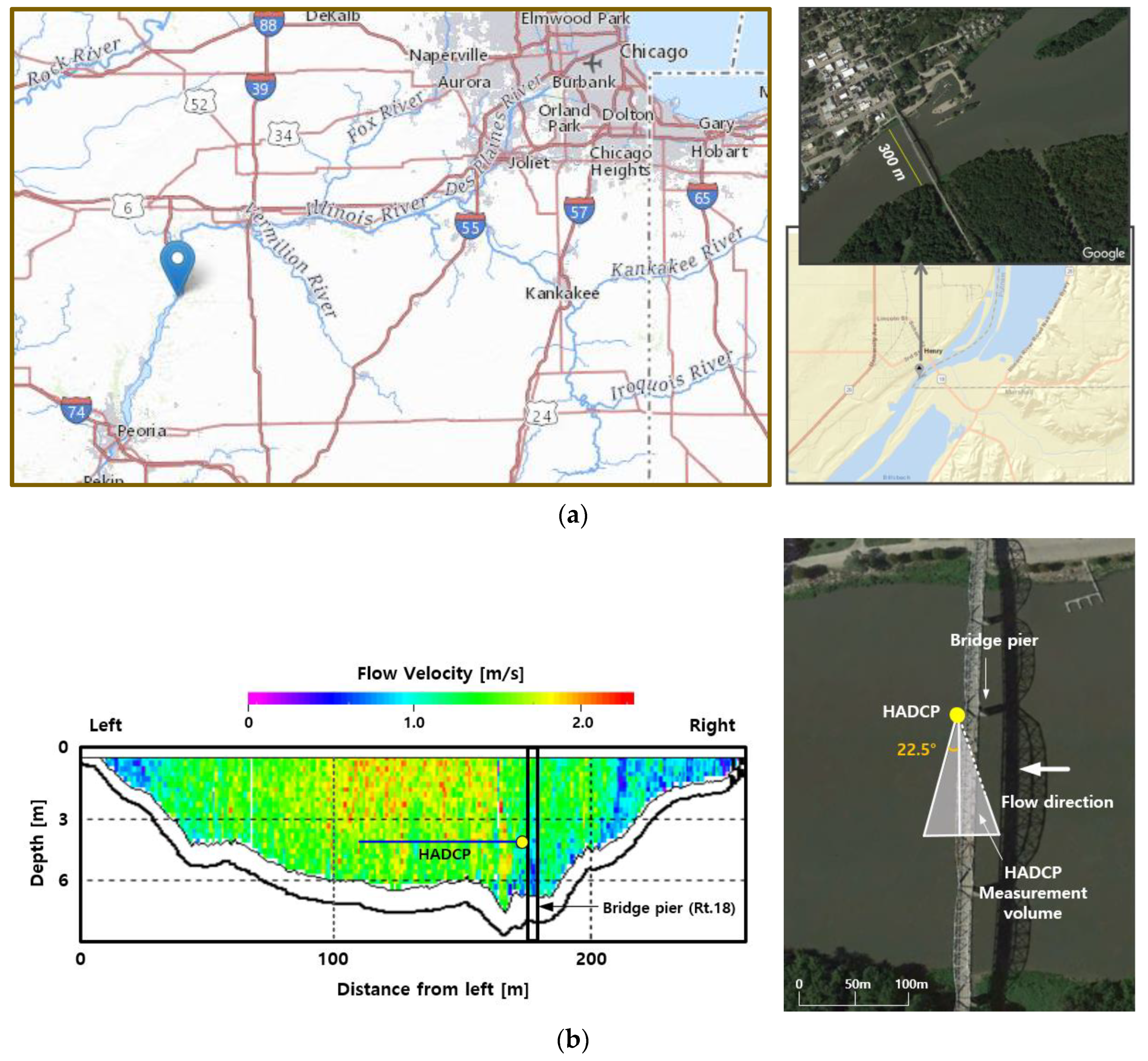
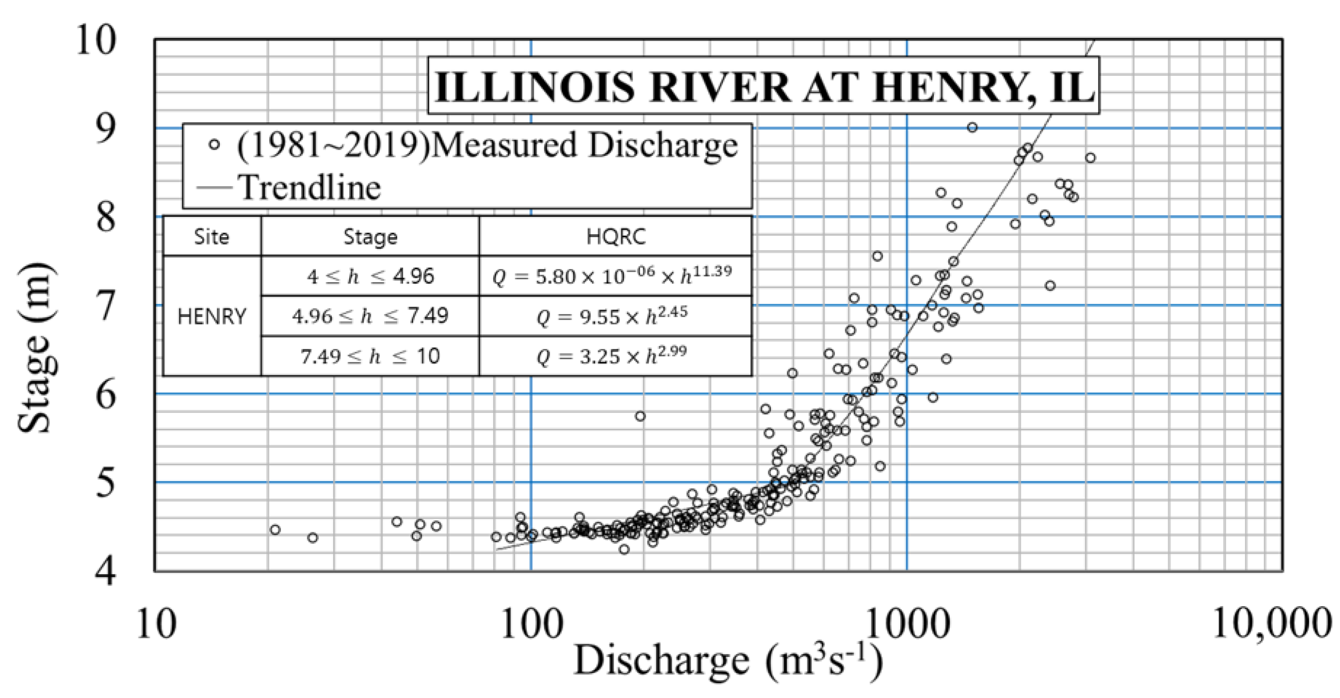
3.1. Study Site

The location of the index-velocity gaging site analyzed in this paper is shown in Figure 2a. The drainages are of the station is 35,078 km2. The station is set on a 2000 m quasi-straight reach of the Illinois River where flood wave propagations is not significantly affected by the presence of man-made structures. The closest river control structures are more than 50 km upstream and downstream from the gage location (i.e., Starved Rock and Peoria lock and dam structures, respectively).
The channel is about 300 m wide and 6 m deep for high flows, and it controls the flow through the station at all stages excepting for low flows near the Peoria Lock and Dam (C. Prater personal communication, 2019). The index velocity is measured with a 1500 kHz SonTek-SL HADCP positioned in the cross-section, as illustrated in Figure 2b. The mean bulk channel velocity is obtained with the regression equations provided in Figure 2b. It can be noted that the length of the HADCP acoustic path is about 55 m (including the blanking distance), covering less than half of the width of the river corresponding to the HADCP elevation. This situation is not uncommon [30], and it often occurs in practice, as finding an optimum location for the probe needs to fulfill multiple requirements (e.g., full probe submersion of the instrument acoustic path, traversing a flow area of maximum possible length without encountering large non-uniformities due to the stream boundary presence). The stage, index velocity, and discharge measured at the gages are transmitted every 15 min to the USGS national streamflow system, which is publicly available. All the data reported in this paper are retrieved from the open-accessible gaging station website. Table 1 provided relations built between discharge and index velocity considering stage.

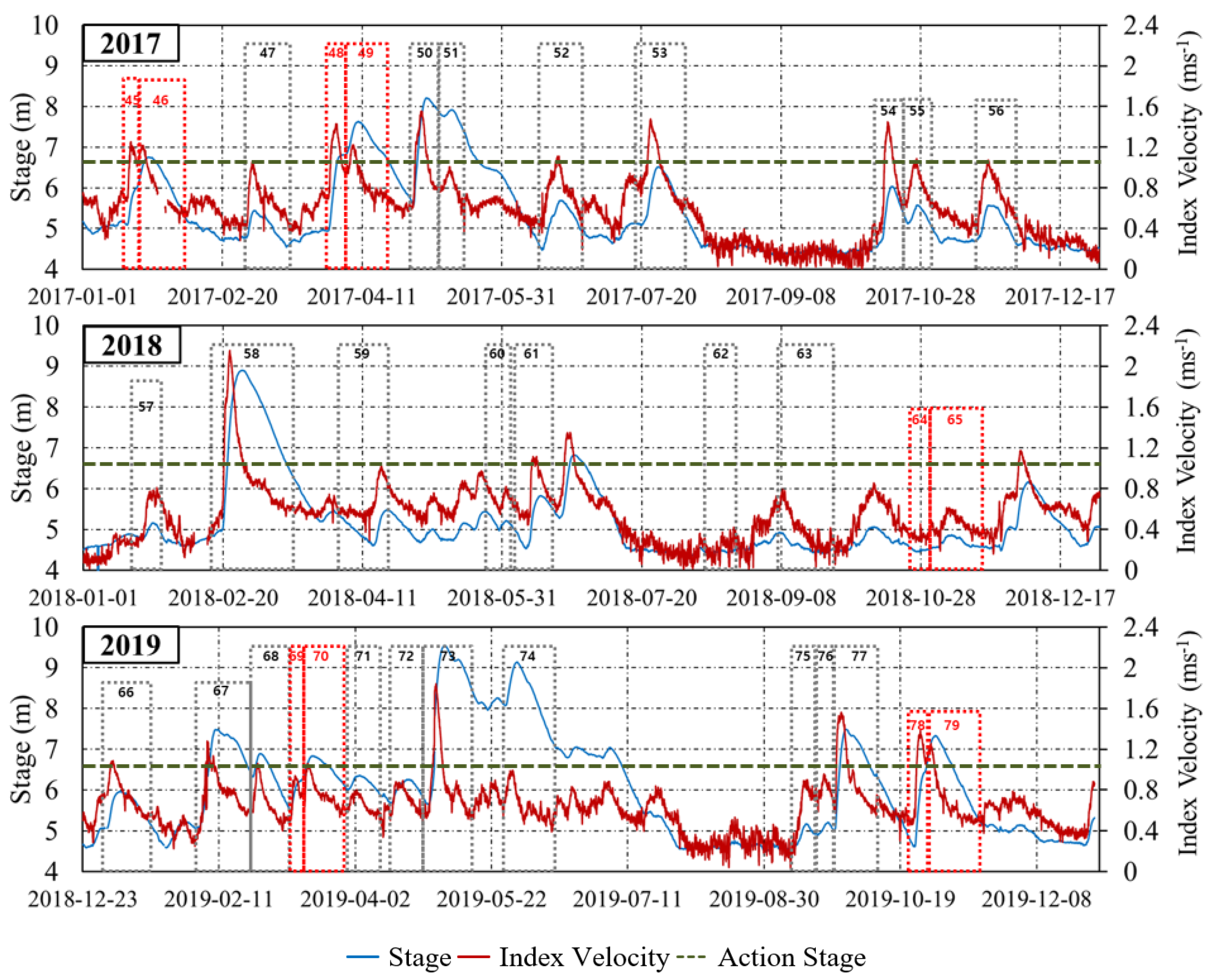
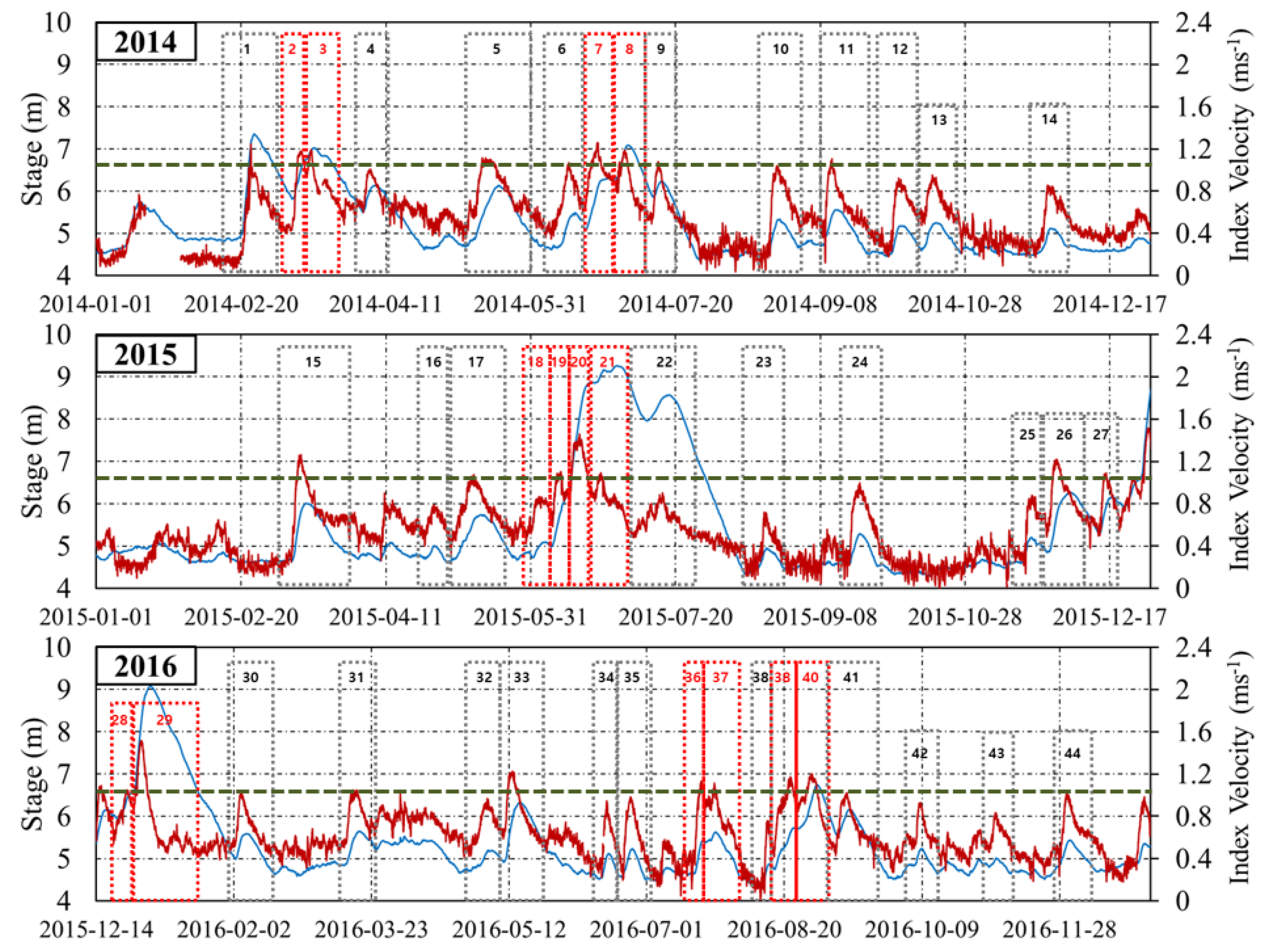
3.2. Monitoring Datasets

Until recently, the hysteretic behavior in the relationships among the flow variables has rarely been captured in natural streams, because the high-temporal resolution instruments capable of measuring simultaneously more than one flow variable were not available. The introduction of the new generation of acoustic profilers at gaging stations has enabled valuable insights into the dynamics of unsteady open-channel flows. One such site is the USGS gaging station #05558300 analyzed herein. Before selecting this site for illustration, we explored the hysteresis presence over six years of data recorded at the station. The implementation of the hysteresis diagnostic formulas developed by Dottori et al. [27], Mishra and Seth [31], and Fread [32] to the available dataset have compellingly confirmed the possibility of developing diffusion and full dynamic waves even for relatively moderate storms propagating through the station [8].
Our illustration starts with time series of stages and index velocities directly measured at this IVRC-based station for the Water Years (WY) 2014 to 2019 (see Figure 3). The time series in this figure allows identifying flood waves propagating through the station alternating with periods of steady flows (baseflow). We define flood wave duration using the National Oceanic and Atmospheric Administration’s (NOAA) terminology, i.e., the contiguous time interval for which the stage is above the one corresponding to baseflow (ncdc.noaa.gov/stormevents). While the most damaging flood impacts are related to the wave peak (i.e., crest), flooding can occur at lower stages, too. To place the magnitudes of the flow waves in the flooding context, we include in Figure 3 the “Action Stage”, which is defined by NOAA’s National Weather Service (https://w1.weather.gov/glossary, accessed on 20 December 2021) as the first flood warning level. When the stream reaches the Action Stage, communities and agencies in charge of flood mitigation typically initiate preparations for flood response activities. Table 2 lists the numerical values for the maximum of the flow variables during the major flood waves (storm events) of WY 2017. We choose WY 2017 as it is a typical water year with the maximum discharge and stage values (i.e., 2600 m3s−1 and 8.20 m) compared with the top discharge and stage values recorded during the 2014–2019 observation interval (i.e., 4560 m3s−1 and 10 m, respectively). It can be noted that out of the eight storm events in the WY 2017, only three exceeded the “Action Stage” level (i.e., 6.7 m).
The visual inspection of the time series for stage and index velocities in Figure 3 reveals several notable features. First, it can be noticed that the time periods taken by flood wave propagation represent a significant part of the annual records. A second, perhaps less expected feature, illustrated in this figure is the easy-to-detect and persistent trend in the time series: the index-velocity peaks precede the stage peaks. This trend is unequivocally related to the hysteresis effect as will be discussed later in the paper. The non-synchronicity of the hydrographs leads to a situation in which, near the hydrograph peak, the index-velocity time series decreases in magnitude while the stage continues to rise for a short time. This is somewhat conflicting with the conventional description of the flood wave propagation where it is assumed that the rising and falling limbs of variable hydrographs are identical.
In order to make the above-mentioned distinction, we use the terms ascending and descending when referring to the index velocity hydrograph “pulses” and the terms rising and falling for stage hydrograph, since these terms are conventionally used. Pulses are defined herein as the groups of consecutive data points recorded on the index-velocity hydrograph pertaining to an acceleration–deceleration cycle [33]. Pulses are related to changes in the rainfall intensity and/or its spatial distribution over the station’s drainage area. As seen in this figure, one storm event can contain a single or multiple pulses. The numbered rectangles in Figure 3 indicate individual storms listed in their chronological order for the observation period. The gradients and magnitudes of the pulses on the rising limb of the stage hydrograph are decisive for determining the severity of the hysteretic loops [34,35]. Severity is used in the present context to indicate the magnitude of the gradients in the changes in the flow variables for a given pulse; the larger the gradients, the more severe the event. The single-pulse storm produces one peak in the stage hydrographs that, in fact, represents the flood crest. For multiple-pulse storm events, the magnitude of the flood crest is impacted by all the pulses occurring on the rising limb of the stage hydrograph.

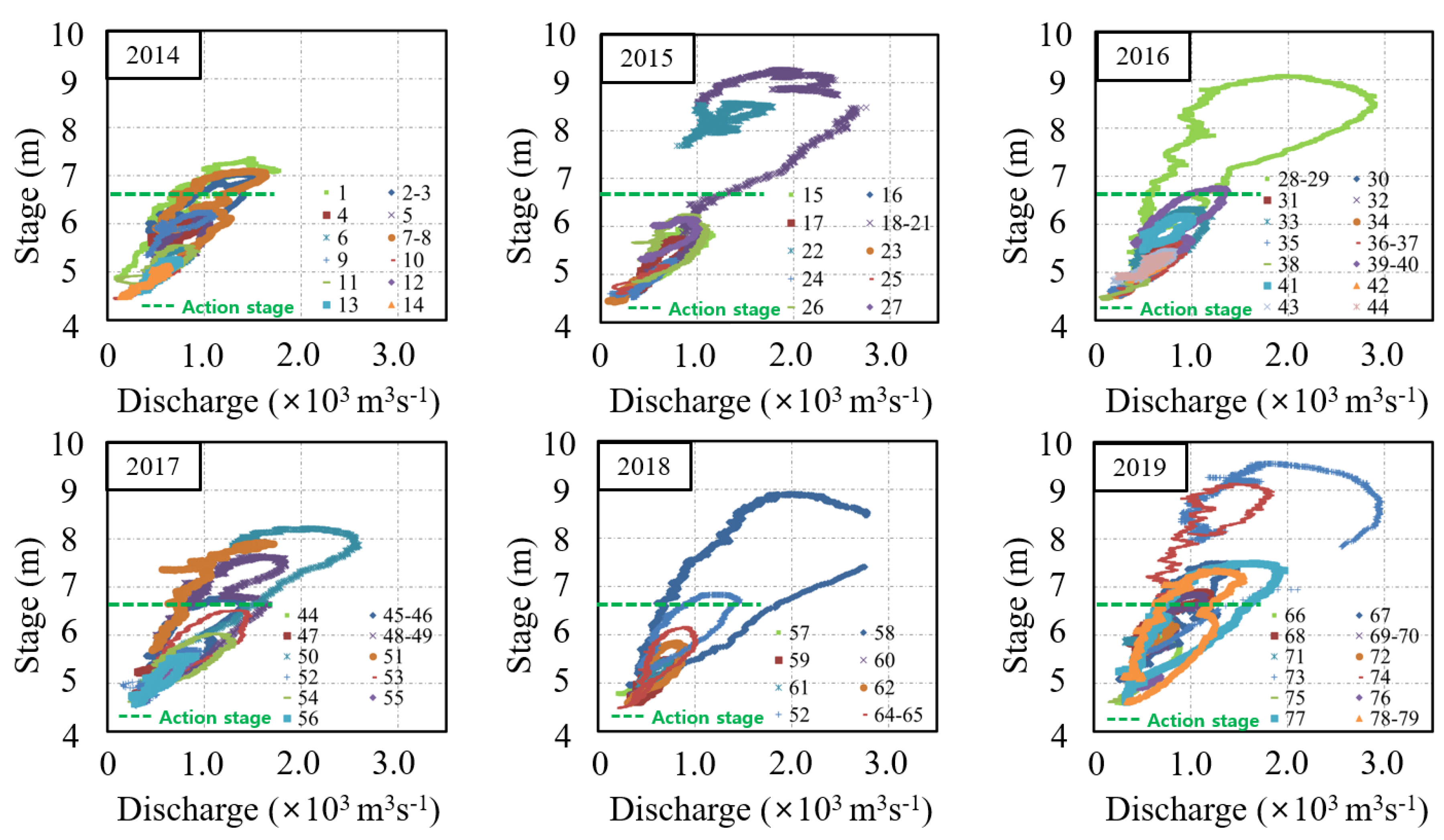
3.3. Substantiation of the Hysteretic Features in the Annual Datasets

The phase difference between the peaks of the index velocity and stage timeseries plotted in Figure 3 is an unmistakable indication of the unsteady flow presence, as for steady flows, the maximum stage coincides with the maximum discharge and bulk flow velocity, as discussed in Figure 1. The trends displayed by the index-velocity hydrographs are the same for the cross-sectional bulk velocity, as the two quantities are related through the one-to-one IVRC relationship for the entire range of flows. Figure 4 displays all the unsteady events within the available dataset plotted in time-independent stage-discharge coordinates to substantiate that each event follows a distinct relationship commensurate with the characteristics of each storm. Collectively, these relationships produce “cloud-like” patterns. Data segments missing in the loops are time intervals when the gaging station temporarily missed or mismeasured data points (typically during high or energic flows). The “Action stage” warning level is also illustrated in this figure to highlight that the flows above this stage are developing the most prominent hysteretic effects.
The hysteretic behavior affects not only the stage-discharge relationship but also those among any two of the other flow variables, as indicated in Figure 5 for the major storms of WY 2017. The cloud of loops for each of the dependencies are bundled along inclined lines of different slopes. The thickness of the cloud and their slope are specific for each relationship. The median slope for each cloud corresponds to the steady-flow relationship for the respective variable pairs. More specifically, we argue that the unsteady flow loops follow the Saint-Venant equation while the steady-flow relationships follow the Manning’s equation that is a sub-component of the first equation [8]. Visual inspection of the plots in Figure 5 indicates that the most prominent impact of hysteresis for this site is associated with the largest storm of the WY 2017, i.e., storm #50 (see Figure 3). For this event, the largest impact of hysteresis can be noted for the stage vs. index-velocity relationship (Figure 4: 60% at 7.5 m), followed by stage-discharge relationship (Figure 5a: 49% at 7.5 m), and index-velocity vs. discharge relationship (Figure 5b: 36% at 1700 m3).

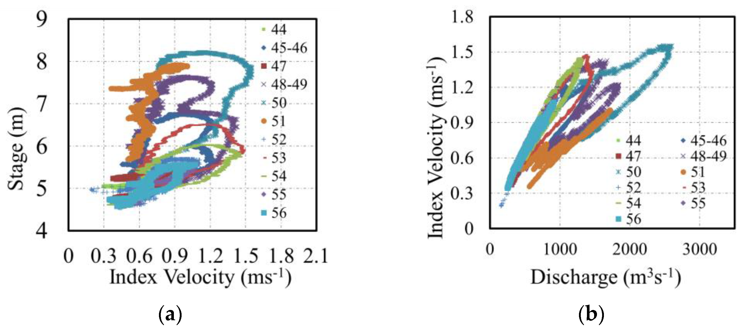
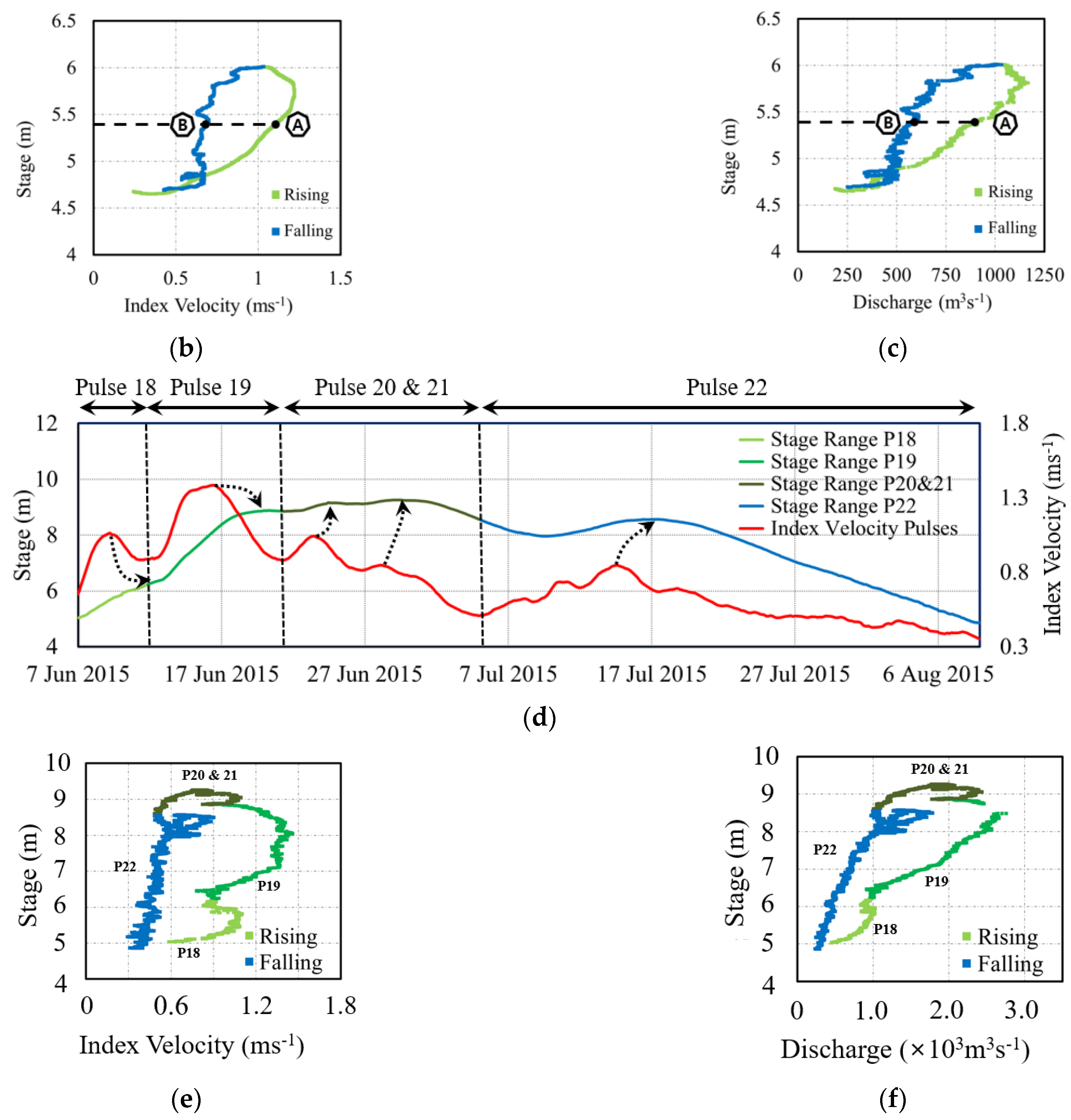
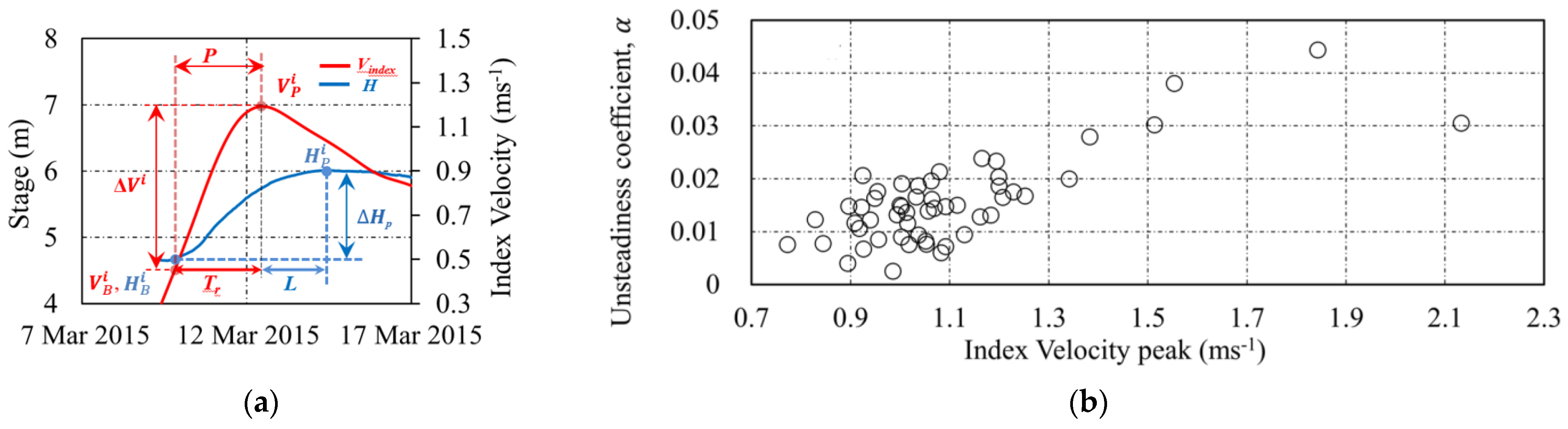
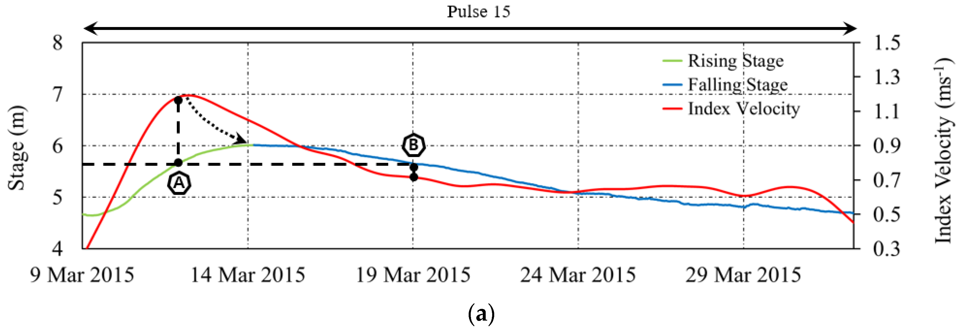
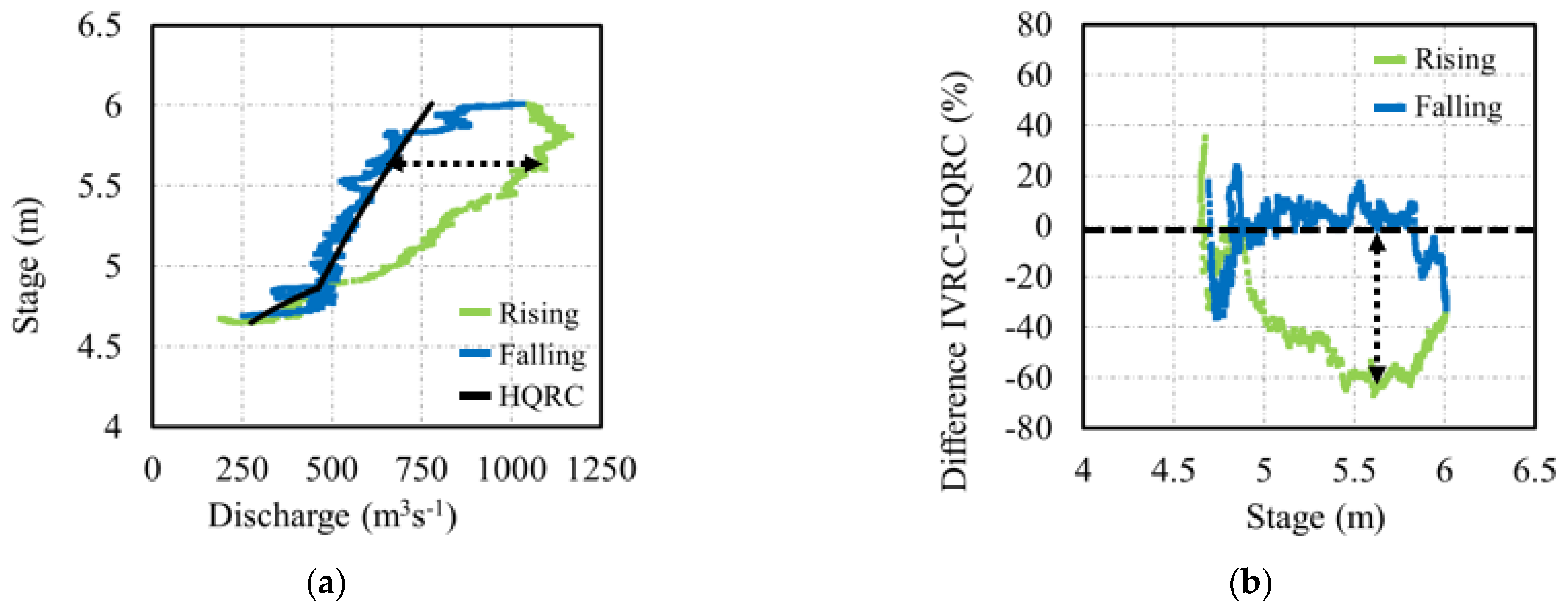
3.4. Substantiation of the Hysteretic Features in Individual Event Datasets

Ensuing from analytical considerations exposed in Muste et al. [8], the hysteresis associated with unsteady flows propagating through a prismatic channel affects the relationships between flow variables in multiple ways, unravelling the unsteady mechanics from several viewpoints. Some of these views and associated relationships are well documented theoretically (e.g., [36]) and through laboratory experiments (e.g., [37]), but they have been rarely captured in natural streams. With the advent of instruments such as HADCPs, we can observe aspects of the flows that were not possible to document in natural conditions before. Taking advantage of the HADCP data for supporting the index method at USGS #05558300 station, we subsequently illustrate various dependencies occurring between flow variables during single-pulse and multiple-pulse storm events (see Figure 6). The data plotted in this figure, as well as for most of the subsequent plots, are smoothened to aid the visualization of the discussed features. A variable-span smoother based on local linear fit [38] was applied to the 5-point averages dataset collected by the HADCP. It should be noted that the index-velocity time series plotted in Figure 6a are acquired across the stream from fixed positions in the vertical, while bulk channel velocity is derived from this velocity via a rating curve; therefore, there are slight differences between the actual loop shapes for the two related variables. However, the two velocities are closely linked; therefore, the trends visualized during the flood wave propagation are similar.
The plots for the single-pulse event in Figure 6a illustrates that the trends in index velocity and stage hydrographs are closely coupled in time but not synchronous. The time separation (i.e., phase shift) of the two variables’ hydrographs leads to different values of the index velocities on the rising and falling limbs for the same depth, as illustrated by points A and B in this figure (and also hinted in the conceptual Figure 1b). The time-independent relationship of the two-directly measured variables is plotted in Figure 6b. The shape of the plot suggests that the flows on the rising and falling limbs of the stage hydrograph display higher velocities during flow acceleration compared with those during decelerated flow. Figure 6c display the often-used representation of the stage-discharge relationship as estimated by the IVRC method for this single-pulse storm event.
Plotted in Figure 6d–f are the same dependencies for a multiple-pulse storm event. While tracing the relationship between the time series for index velocity and stage in Figure 6d is more intricate, a careful inspection of the changes in the time series for the two variables allows us to identify the effect of each individual index-velocity pulse on the stage variation. This impact is visually represented in Figure 6d either as a local stage peak or just as an inflexion point in the stage time series, as indicated with arrows in this figure. Individual pulses contain both ascending and descending phases; hence, we label them as sub-storms contained within the overall storm event (from base flow and back). Each sub-storm produces distinguishable loops within the overall large loop of the multi-pulse storm event, as illustrated in the Figure 6e,f.
Figure 4, Figure 5 and Figure 6 provide abundant experimental evidence that the hysteretic behavior is materialized through the presence of loops in the time-independent relationships and through a detectable “decoupling” of the flow variable hydrographs in the time-dependent graphical representations. Another feature of interest for characterizing the hysteretic behavior is its severity. One of the built-in factors in determining the hysteresis severity is the slope of the channel bed at the site, with milder slopes producing more severe hysteresis [8]. For the same site, the magnitude of the loops and time lags between hydrographs are determined by the severity of the storm events (i.e., proportional to the gradients for the flow changes), as shown in the measurement summaries presented in Figure 4 and Figure 5. We argue herein that the pulses of unsteady flow with the same starting point, index-velocity magnitude, and gradient on the rising limb of the stage hydrograph produce identical hysteretic loops for a given site, whether the event is single- or multi-pulse.
Quantification of the storm severity in this discussion is made using the unsteadiness coefficient proposed by Nezu et al. [39]. According to this study, this coefficient is proportional to the lag between the maximum shear stress (that is highly correlated with the maximum velocity peak) and the maximum depth (i.e., stage peak). Assuming a hydrostatic pressure distribution, the unsteadiness coefficient is defined by the ratio between the rising speed of the water surface and the celerity of the propagation wave. Consequently, the severity of a single-pulse event can be defined as:
α = H P i H B i T r × 2 V B i + V P i
where α is the unsteadiness coefficient, P defines pulses, Vi is the index velocity, Tr is time duration for the index velocity pulse to reach its peak, L, is the time duration (lag) between the index velocity peak and the associated stage peak, Hi; indices “B” and “P” stand for the base and peak of individual pulses (see Figure 7a). Equation (1) can be applied to individual pulses within multi-pulse events by accounting for the state of the variables at their base and peak for each pulse [40]. The relationship between the index-velocity peak and its severity for all the pulses in the dataset used herein is plotted in Figure 7b.
Using the aforementioned considerations, we illustrate in Figure 8 the importance of the hysteresis severity on the impact produced on the variables’ dependencies. The time-independent and time-dependent plots in this figure contain all the flow variables measured and estimated at this USGS station, as reported on the publicly accessible site. The numerical values of the unsteadiness coefficients for each storm are also indicated in this figure. The plots on the left side of Figure 8 indicate, as expected, that the magnitude and thickness of the hysteresis are connected. Specifically, the smaller the stage variation for a specific storm event, the thinner the hysteretic loop. This is actually one of the reasons invoked for overlooking hysteresis in current monitoring practice, because while the hysteresis loops are always present, they cannot be distinguished from the measurement uncertainty at low flows. Unfortunately, most of the calibration/validation of the ratings are acquired at low flows, where hysteresis is less observable [20]. The study conducted by Muste and Kim [41] demonstrated using direct measurements at this station that quasi-equal magnitude pulses produce larger loops if the storms are more severe (sharper peaks in the index-velocity time series) and that equal-severe storms produce thicker loops if the index-velocity peak is of larger magnitude. It is obvious that storms that are both large and severe display commensurately larger loop thickness and lag time between the index-velocity and stage hydrographs.
Another relevant impact of the hysteresis severity is that the larger loops are associated with larger hydrograph separations, as indicated by the plots on the right side of Figure 8. It is also notable that the hydrograph peaks follow systematically the same succession, i.e., index-velocity peaks occur first followed by the discharge and stage peaks. This inherent unsteady flow property was used by these authors to develop a short-term forecasting algorithm using the peak of the index-velocity as a triggering point for forecasting [40].

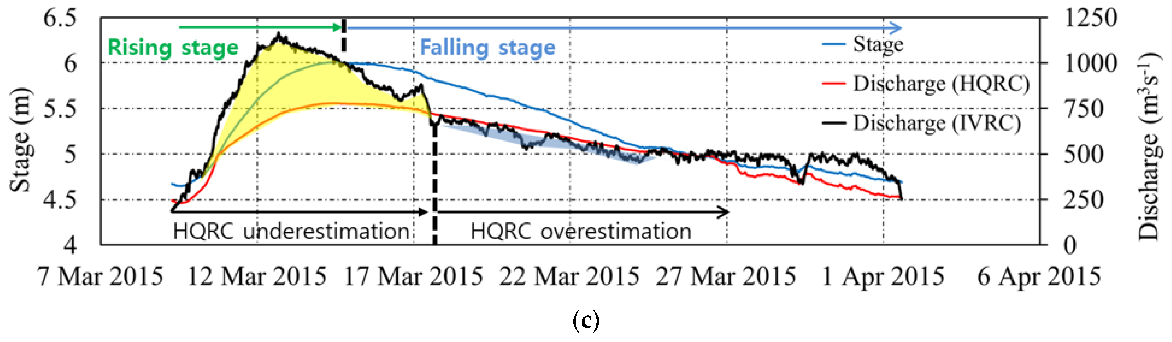
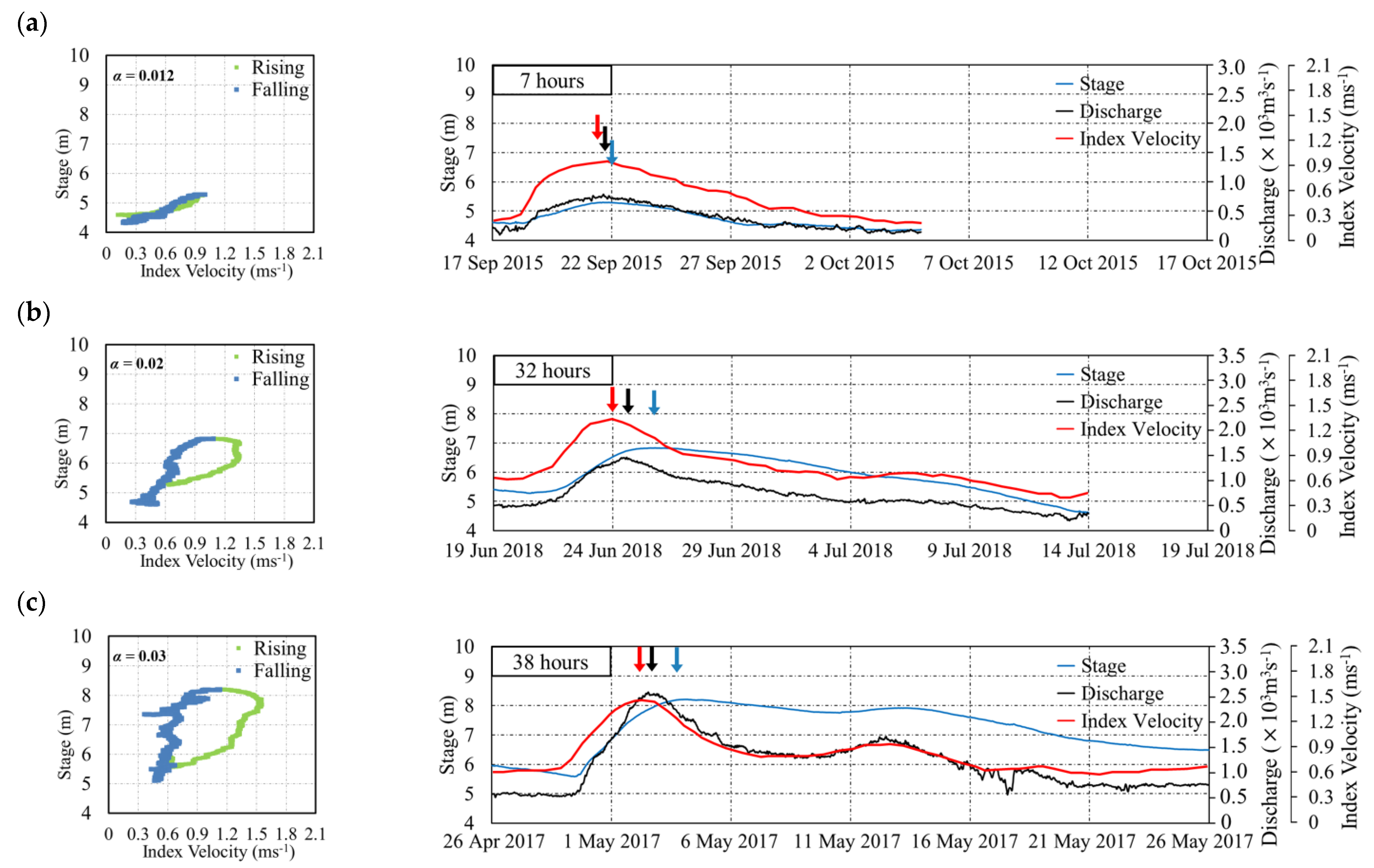
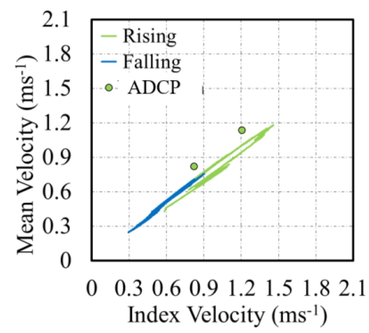
3.5. IVRC Performance during Flood Wave Propagation

A subject of great interest for the present context is the evaluation of the improvement brought by the IVRC method over the HQRC when operating in unsteady flows at a site exposed to hysteresis. Given that for the present analysis, there are neither stage-discharge relationships nor direct discharge measurements taken over the whole duration of a storm, we cannot provide the much-needed comparison. To enable such a comparison, we developed a “surrogate” HQRC rating using the direct measurements acquired for developing the IVRC rating and validating it after its construction. A total of 253 such direct measurements were acquired between 1981 and 2019 for this site (C. Prater personal communication, 2019). The surrogate HQRC shown in Figure 9 was constructed using the directly measured discharges paired with the corresponding stages. Furthermore, we determined distinct regression equations for the low-, medium-, and high-stage ranges, as recommended by best practice guidelines [14]. We realize that such an obtained HQRC rating does not strictly follow the intricate graphical construction used by USGS to develop stage-discharge ratings, but we consider this surrogate sufficient for the present discussion.
Figure 10a illustrates essential features of the IVRC-HQRC comparison using the stage-discharge relationship commonly used by the hydrometric community to demonstrate hysteresis presence. The storm chosen for comparison is event #15 of the WY 2015 that does not display the largest stage in the analyzed dataset, but it is one of the most intense, as proven by the sharp increase in the index-velocity illustrated in the time-series of the WY 2015 illustrated in Figure 3. The first comment on Figure 10a is the considerable departure of the IVRC estimated values from those of HQRC, i.e., up to 60% on the rising limb of the stage hydrograph, as illustrated by the arrow added in Figure 10b. The second comment is that the HQRC data fall closely to the datapoints on the falling limb of the IVRC estimates. This feature was also noted by the authors in previous studies at other IVRC-based gaging sites (e.g., [20,23]). The most likely explanation for this feature is that while on the rising stage, the flow is marked by a sudden acceleration, on the falling limb, the deceleration of the flow is slower. For this site, the ratios between falling and rising times are anywhere between 4 and 15. We perceive the slower deceleration on the falling limb as being akin to a series of successive step-like steady flows of continuously decreased discharges, therefore being closer to the shape described by a steady HQRC.
Additional inferences can be drawn from the comparison of the time-dependent plots of the discharges estimated by the IVRC and HQRC methods. The stage hydrograph is added in this figure for delineating the rising and falling limbs as defined in the present discussion. The plots in this figure reveal two new inferences. The first one is that the IVRC discharge peak estimate is 8% larger than the one predicted with the HQRC rating. Differences up to 15% between actual flows measured at the site and HQRC estimates were reported by Jarrett [42] and Di Baldassarre and Montanari [19]. Along the same line, Fenton and Keller [43] as well as Henderson [7] explain analytically that the maximum discharge of diffusive flood waves is larger (and occurs earlier) than the flow computed from simple HQRC ratings. An additional factor toward the generalization of this first inference is the fact that the reliability of any type of rating in the higher flow range area is not as robust as for lower flow range, as the density of the calibration/verification measurements is less dense for high flows. The second inference is that the discharges on the rising limb are considerably underestimated by the HQRC method and are not fully compensated over the remaining period of flood wave propagation. While the IVRC and HQRC features are significant and consistent in this study, the numerical values associated with the differences between the two methods cannot be generalized for other sites and types of waves propagating through hysteresis-prone gaging stations.

4. Discussion

The hysteretic behavior at the site of the presented case study is mostly dominated by flow unsteadiness without significant contributions from other potential causes that can lead to hysteresis (e.g., effects of instream vegetation, bedform-induced roughness development, and baseflow–stream interactions). Rantz et al. [14] labels this situation as the one where the energy slope is mostly changed by the variation in discharge to distinguish from the situations when the slope change is mostly driven by the variable backwater. Often, the two effects are both involved. Furthermore, our discussion assumes that the flood wave propagation occurs in channels predominantly controlled by friction, whereby the dominant energy losses are due to channel boundary roughness rather than changes in the channel geometric features (local control) [12]. Moreover, we discuss herein hysteresis impacts for water elevation in the channel that are less than the bankful stage (i.e., as flood stage). When this stage is exceeded, additional flow complexities occur as the mass and momentum exchanges between the main channel and floodplain impede a straightforward interpretation of the hysteretic effects. Finally, it is assumed that there are no issues related to instrumentation deployment and operation, as these factors can also impact the interpretation of the measurements when the sensor positioning and time synchronization are not properly performed. Under the aforementioned conditions, and in the absence of a demonstrable presence of backwater effects, the hysteresis features can be solely attributed to the flow unsteadiness.
While the illustrations of the present study confirm previous conclusions that IVRC better capture unsteady flows, the majority of the discussions in this paper are focused on the exploration of essential features of the hysteretic behavior as reflected by the data collected at an operational IVRC gaging station. The presented results unequivocally demonstrate that the IVRC method: (a) provides distinct relationships between flow variables for the rising and falling limbs of the hydrographs, (b) captures the sequencing of the measured variable hydrographs, which is a feature that is inherent if item (a) above is substantiated at a given site [41], (c) substantiates that the changes in the thickness of the loops and associated hydrograph phasing are commensurate with the magnitude and severity of the hydrographs, and (d) substantiates significant differences in the discharges estimated with the HQRC method.
As mentioned above, the datasets available for the present study do not contain a suitable benchmark to allow a thorough assessment of the IVRC or HQRC performance in steady and unsteady flows. Such benchmark datasets are ideally acquired with high-accuracy alternative instruments, rigorous protocols, and prescribed flow conditions. The latter conditions can be only attained at sites where the river flow can be controlled, and measurements can be repeated a few times to capture the variability of the in-situ conditions. The closest alternative to such an ideal assessment scenario is the acquisition of direct measurements using ADCPs continuously operated in steady and unsteady flows. The above considerations highlight why the IVRC-HQRC performance assessment is difficult to come by and rarely executed. One of these rare studies was, however, conducted by the present authors at a USGS gaging station in Idaho where the flow could be controlled and repeated under the same conditions [44]. In this study, we analyzed data from routine and controlled experiments to illustrate the IVRC and HQRC performance in evaluating streamflow over a range of flow regimes by comparing the monitoring methods’ estimates with the measurements acquired with a Winter–Kennedy Meter that are calibrated to relate the pressure losses in the turbine casing to the discharge through the turbine [45]. The WKMs were installed in the hydropower plant’s turbine housing located immediately upstream from the gaging station. While we are aware that these conclusions cannot be readily extended to other locations, we deem that it is useful to cite these results in the present context.
The evaluation of the Idaho dataset showed that the flow estimates obtained with the two monitoring methods during steady flows were within 5% from the estimates provided by the WKM. For unsteady flows, it was found that the IVRC method was overall superior to the HQRC performance, but there were differences up to 40% between the IVRC discharge estimates and those provided by WKM during the highest flow-change rates. These large differences were attributed to the fact that the flow changes were considerable in magnitude for both rising and falling phases (from simple to double), and they were made over short durations (less than an hour). Such flow changes are quite typical for hydropower plants where the turbines are set on and off during the day to accommodate the energy consumption in the power distribution grid. There are no specific reasons to expect that the Illinois River dataset analyzed in the present study is widely different in term of overall findings from the Idaho study because the protocols for constructing and using the rating curves are uniformly applied at all USGS gaging stations. Actually, similar findings were inferred by the authors from another IVRC study on controlled flood waves at a gaging station located in Spain [20].
The presented experimental evidence allows us to further explore some issue regarding the IVRC rating construction that are still unsettled. Currently, most of the IVRC ratings are constructed with protocols that do not distinguish between the hydrograph flow phases, similar to the protocols used in stage-discharge approaches. In this approach, the statistical analyses are applied to the whole calibration dataset for establishing one-to-one regression lines that fit best the available data points. The obtained regressions are used for all flow regimes. Similar to HQRC, the graphical construction involves subjective decisions on the parameters and thresholds used in the analysis. In the absence of robust understanding of the flow dynamics or experimental evidence, the use of statistical analyses alone precludes to state when the analysis outcomes are good enough or if the observed disagreements are not merely reflections of the unknown physics processed with statistical tools.
Use of the one-to-one IVRC protocols for the USGS Henry station led to the conclusion that the multiple-linear regression for the IVRC regressions equation was adequate from June 2015 to February 2018. After this date, a simple linear regression was adopted (see Table 1). The graphical representation of the IVRC ratings using the equations in Table 1 are plotted in Figure 11 for the single-pulse events illustrated in Figure 8. It can be noticed that while for the smaller storms, the rating does not show a clear distinction between the rising and falling stage, for the largest storm (i.e., event #50 in 2017), there is a perceptible and consistent differentiation of the IVRC rating for the rising and falling stages. The thickness of the hysteresis loop in the IVRC for the largest flow events is considerably smaller than that in the stage-discharge relationships shown in Figure 4. Similar findings have been observed through other studies (e.g., [23,46]), therefore signaling the need to further explore the validity of the unicity of the IVRC relationship for all flow regimes.
In an attempt to test the adequacy of the one-to-one relationship for the IVRC rating during unsteady flows at the Illinois station, an additional check is made using the mean bulk velocities determined from the direct ADCP measurements acquired for validation of the IVRC rating between 2015 and 2018. During this interval, there are 19 ADCP validation measurements, among which only three measurements are taken at stages above the Action Stage indicated in Figure 3. Two of these measurements were acquired during the propagation of Pulses 20 and 21. The comparison between the IVRC rating estimates with the directly measured mean velocity via ADCP is plotted in Figure 12. It can be noted from this figure that the ADCP velocities (acquired on the ascending limb of the stage hydrograph) show larger values than those estimated with the IVRC rating. These differences seem to indicate that the construction of the IVRC relationship using separate relationships for the rising and falling phases of the stage hydrograph is a better alternative than the one-to-one approach provided in Table 1. Definitely, a thorough assessment of this argument requires further analyses on considerable larger datasets of this kind.

5. Conclusions

The fresh perspectives on the IVRC measured flow variables presented in this paper provide useful insights into the physics of flood wave propagation in natural open channels that are often overlooked in routine monitoring. The experimental evidence presented in this study indicate that:
(a)
Hysteresis occurring at monitoring sites located in low-gradient channels exposed to flood waves is significant, being commensurate with the site and flood wave characteristics;
(b)
Unsteady flows produce a non-unique relationship between any two of the flow variables and an out-of-phase flow hydrographs during the flood wave propagation;
(c)
The index-velocity method can more aptly capture hysteresis compared with the stage-discharge method;
(d)
If a discharge monitoring method capture hysteresis, it is implicit that it can also distinguish the peak sequencing and vice versa.
Given that the above findings are based on only a limited dataset, the outcomes of the discussion should be regarded as being indicative rather than confirmative. However, it is our hope that the outcomes of the present study indicate that the effect of hysteresis on monitoring methods requires additional research.
The present study convincingly demonstrates that the acoustic probes such as HADCPs are reliable instruments for providing valuable data and insights in complex measurement situations. The use of directly measured data provided by these instruments are valuable benchmark datasets that can uniquely support multi-purpose investigations based on analytical, data-driven, and numerical simulations. The capabilities of the new generation of instruments can underpin better decision making in water resource management and flood mitigation efforts and open possibilities to use the produced data in novel ways for enhanced scientific investigations in streams and rivers.

Author Contributions

The conceptualization and data processing methodology were developed by M.M. and D.K. The data processing, analysis, and presentation were carried out by K.K. All authors have read and agreed to the published version of the manuscript.

Funding

Most of the illustrations in this paper are outcomes of a research study conducted for SonTek/YSI (I556800-C) by the paper’s authors. Center. The first author acknowledges the partial support offered the NSF EAR-HS 2139649 award. The second and third authors were partially funded by Basic Science Research Program through the National Research Foundation of Korea (NRF) funded by the Ministry of Education (2021R1F1A1060295).

Data Availability Statement

Datasets supporting the illustrations presented above will be assembled in an open-access drive for consultation with interested readers.

Acknowledgments

Discussions with Janice Yasui and Xue Fan of SonTek/YSI enriched the horizon of analysis. The analysis presented in this paper have greatly benefitted by constructive discussions with R. Jackson and R. Holmes and additional data offered by J. Duncker, C. Prater, and R. Beaulin with the US Geological Survey Midwest Water Science Center.

Conflicts of Interest

The authors declare no conflict of interest.

References

  1. USGS. A history of the Water Resources Branch, U.S. Geological Survey; Follansbee, R., Ed.; Volume I, from Predecessor Surveys to 30 June 1919; U.S. Geological Survey: Denver, CO, USA, 1994.
  2. Jain, S.; Lall, U. Magnitude and timing of annual maximum floods: Trends and large-scale climatic associations for the Blacksmith Fork River, Utah. Water Resour. Res. 2000, 36, 3641–3651. [Google Scholar] [CrossRef]
  3. Holmes, R.R. River rating complexity. In Proceedings River Flow Conference; Taylor & Francis Group: St. Louis, MO, USA, 2016; ISBN 978-1-138-02913-2. [Google Scholar]
  4. Saint-Venant, A.J.C. Théorie du mouvement non permanent des eaux, avec application aux crues des rivières et a l’introduction de marées dans leurs lits. Comptes Rendus L’académie Sci. 1871, 73, 147–154, Discussion 237–240. [Google Scholar]
  5. Chow, V.T. Open Channel Flow; McGrow Hill: New York, NY, USA, 1959. [Google Scholar]
  6. Hunt, A.E. The Behaviour of Turbulence in Unsteady Open Channel. Ph.D. Thesis, University of Canterbury, Christchurch, New Zealand, 1997. [Google Scholar]
  7. Henderson, F.M.; Open Channel Flow. Macmillan Series in Civil Engineering; Macmillan Company: New York, NY, USA, 1966; p. 522. [Google Scholar]
  8. Muste, M.; Lee, K.; Kim, D.; Bacotiu, C.; Oliveros, M.R.; Cheng, Z.; Quintero, F. Revisiting hysteresis of flow variables in monitoring unsteady streamflows. J. Hydraul. Res. 2020, 58, 867–887. [Google Scholar] [CrossRef]
  9. Ponce, V.M. Development of Physically based Coefficients for the Diffusion Method of Flood Routing; Contract No. 53-3A75-3-3; U.S. Soil Conservation Service: Lanham, MD, USA, 1983.
  10. Ferrick, M.G. Analysis of River Wave Types. Water Resour. Res. 1985, 21, 209–220. [Google Scholar] [CrossRef] [Green Version]
  11. Aricò, C.; Nasello, C.; Tucciarelli, T. Using unsteady-state water level data to estimate channel roughness and discharge hydrograph. Adv. Water Resour. 2009, 32, 1223–1240. [Google Scholar] [CrossRef]
  12. WMO. Manual on stream gauging, Volume I, Field Work; World Meteorological Organization Report WMO No. 1044. 2010. Available online: www.wmo.int/pages/prog/hwrp/publications/stream_gauging/1044_Vol_I_en.pdf (accessed on 20 December 2021).
  13. Muste, M.; Hoitink, T. Measuring Flood Discharge. In Oxford Research Encyclopedia of Natural Hazard Science; Subject: Case Studies, Risk Assessment, Vulnerability, Floods; Oxford University Press: Oxford, UK, 2017. [Google Scholar] [CrossRef]
  14. Rantz, S.E. Measurement and Computation of Streamflow; US Geological Survey Water Supply Paper 2175, Vol.1 and 2; US Department of the Interior, Geological Survey: Reston, VA, USA, 1982.
  15. Herschy, R. Streamflow Measurement, 3rd ed.; Taylor & Francis: Oxford, UK, 2009. [Google Scholar]
  16. Levesque, V.A.; Oberg, K.A. Computing Discharge Using the Index Velocity Method; U.S. Geological Survey Techniques and Methods 3–A23; U.S. Geological Survey: Reston, VA, USA, 2012; 148p. Available online: http://pubs.usgs.gov/tm/3a23/ (accessed on 20 April 2020).
  17. Rennie, C.; Hoitink, A.J.F.; Muste, M. Chapter 6 in Experimental Hydraulics; Aberle, J., Rennie, C.D., Admiraal, D.M., Muste, M., Eds.; Taylor & Francis: New York, NY, USA, 2017; Volume II. [Google Scholar]
  18. Faye, R.E.; Cherry, R.N. Channel and Dynamic Flow Characteristics of the Chattahoochee River, Buford Dam to Georgia Highway 141; Geological Survey Water-Supply Paper 2063; U.S. Government Printing Office: Washington, DC, USA, 1980.
  19. Di Baldassarre, G.; Montanari, A. Uncertainty in river discharge observations: A quantitative analysis. Hydrol. Earth Syst. Sci. 2009, 13, 913–921. [Google Scholar] [CrossRef] [Green Version]
  20. Muste, M.; Lee, K. Evaluation of Hysteretic Behavior in Streamflow Rating Curves. In Proceedings of the 2013 IAHR Congress, Chengdu, China, 8–13 September 2013; Tsinghua University Press: Beijing, China, 2013. [Google Scholar]
  21. Schmidt, A.R. Analysis of Stage-discharge Relations for Open Channel Flows and their Associated Uncertainties. Ph.D. Thesis, University of Illinois at Urbana-Champaign, Champaign, IL, USA, 2002. [Google Scholar]
  22. Morlock, S.E.; Nguyen, H.T.; Ross, J. Feasibility of Acoustics Doppler Velocity Meters for the Production of Discharge Records from U.S. Geological Survey Stream-Flow-Gaging Stations; U.S.G.S. Water-resources Investigations Report; USGS: Indiannapolis, IN, USA, 2002.
  23. Cheng, Z.; Lee, K.; Kim, D.; Muste, M.; Vidmar, P.; Hulme, J. Experimental Evidence on the Performance of Ratting Curves for Continuous Discharge Estimation in Complex Flow Situations. J. Hydrol. 2019, 568, 959–971. [Google Scholar] [CrossRef]
  24. Le Coz, J.; Pierrefeu, G.; Paquier, A. Evaluation of river discharges monitored by a fixed side-looking Doppler profiler. Water Resour. Res. 2008, 44, 1–13. [Google Scholar] [CrossRef] [Green Version]
  25. Jackson, P.R.; Johnson, K.K.; Duncker, J.J. Comparison of Index Velocity Measurements Made with a Horizontal Acoustic Doppler Current Profiler and a Three-Path Acoustic Velocity Meter for Computation of Discharge in the Chicago Sanitary and Ship Canal Near Lemont, Illinois; U.S. Geological Survey Scientific Investigations Report. 2011–5205; US Department of the Interior, US Geological Survey: Reston, VA, USA, 2012; 42p.
  26. Kennedy, E. Discharge Ratings at Gaging Stations; US Geological Survey Techniques of Water-Resources Investigations, Book 3, Chap. A10; U.S. Geological Survey: Reston, VA, USA, 1984; 59p.
  27. Dottori, F.; Martina, M.L.V.; Todini, E. A dynamic rating curve approach to indirect discharge measurement. Hydrol. Earth Syst. Sci. 2009, 13, 847–863. [Google Scholar] [CrossRef] [Green Version]
  28. SonTek/YSI. Acoustic Doppler Profiler Principles of Operation; SonTek/YSI: San Diego, CA, USA, 2000; 28p. [Google Scholar]
  29. Ruhl, C.A.; Simpson, M.R. Computation of Discharge Using the Index-Velocity Method in Tidally Affected Areas; Scientific Investigations Report 2005-5004; U.S. Geological Survey: Reston, VA, USA, 2005. [Google Scholar]
  30. Hoitink, A.J.F. Monitoring and analysis of lowland river discharge. In Proceedings of the River Flow Conference, IAHR, Lyon, France, 5–8 September 2018. [Google Scholar] [CrossRef] [Green Version]
  31. Mishra, S.K.; Seth, S.M. Use of hysteresis for defining the nature of flood wave propagation in natural channels. Hydrol. Sci. J. 1996, 41, 153–170. [Google Scholar] [CrossRef]
  32. Fread, D.L. Channel Routing; Anderson, M.G., Burt, T.P., Eds.; Hydrological Forecasting; Wiley: New York, NY, USA, 1985. [Google Scholar]
  33. Muste, M.; Kim, D.; Kim, K.; Ehab, M. Monitoring streamflow pulses. In Proceedings of the 39th IAHR World Congress, Granada, Spain, 19–24 June 2022. [Google Scholar]
  34. De Sutter, R.; Verhoeven, R.; Krein, A. Simulation of sediment transport during flood events: Laboratory work and field experiments. Hydrol. Sci. J. 2001, 46, 599–610. [Google Scholar] [CrossRef]
  35. Mrokowska, M.M.; Rowiński, P.M. Impact of Unsteady Flow Events on Bedload Transport: A Review of Laboratory Experiments. Water 2019, 11, 907. [Google Scholar] [CrossRef] [Green Version]
  36. Kozak, M. A Szabadfelsonu Nempermanens Vizmozgasok Szamitasa; Academia Kiado: Budapest, Hungary, 1977. [Google Scholar]
  37. Graf, W.; Qu, Z. Flood hydrographs in open channels. In Proceedings of the Institution of Civil Engineers-Water Management; Thomas Telford Ltd.: London, UK, 2004; Volume 157, pp. 45–52. [Google Scholar] [CrossRef]
  38. Friedman, J.H. A Variable Span Smother; Technical Report PUB-3477; Laboratory for Computational Statistics, Stanford University: Stanford, CA, USA, 1984. [Google Scholar]
  39. Nezu, I.; Kadota, A.; Nakagawa, H. Turbulent Structure in Unsteady Depth-Varying Open-Channel Flows. J. Hydraul. Eng. 1997, 123, 752–763. [Google Scholar] [CrossRef]
  40. Muste, M.; Kim, D.; Kim, K. A flood-crest forecast prototype for river floods using only in-stream measurements. Commun. Earth Environ. 2022, 3, 1–10. [Google Scholar] [CrossRef]
  41. Muste, M.; Kim, D. Augmenting the Operational Capabilities of SonTek/YSI Streamflow Measurement Probes. Sontek/YSI-IIHR Collaborative Research Report. 2020. Available online: https://info.xylem.com/rs/240-UTB-146/images/augmenting-capabilities-sontek-probe.pdf (accessed on 20 December 2021).
  42. Jarrett, R.D. Errors in slope-area computations of peak discharges in mountain streams. J. Hydrol. 1987, 96, 53–67. [Google Scholar] [CrossRef]
  43. Fenton, J.D.; Keller, R.J. The Calculation of Streamflow from Measurement of Stage; Technical Report; Cooperative Research Centre for Catchment Hydrology and Centre for Environmental Applied Hydrology, Department of Civil and Environmental Engineering, The University of Melbourne: Melbourne, Australia, 2001. [Google Scholar]
  44. Muste, M.; Cheng, Z.; Vidmar, P.; Hulme, J. Considerations on Discharge Estimation Using Index-Velocity Rating Curves. In Proceedings of the 36th IAHR World Congress, The Hague, The Netherlands, 28 June–3 July 2015. [Google Scholar]
  45. ASME. Hydraulic Turbines and Pump-Turbines; Power Test Code (PTC)—18-2011; American Society of Mechanical Engineers (ASME): New York, NY, USA, 2011. [Google Scholar]
  46. Nihei, Y.; Kimizu, A. A new monitoring system for river discharge with horizontal acoustic Doppler current profiler measurements and river flow simulation. Water Resour. Res. 2008, 44, 1–15. [Google Scholar] [CrossRef] [Green Version]
Figure 1. Outcomes of the conventional monitoring methods when measurements were conducted during unsteady flows (adapted from [8]): (a) stage-discharge method (HQRC) and (b) index-velocity method (IVRC).
Water 14 01380 g001
Figure 2. USGS gaging station #05558300 on Illinois River, at Henry (IL): (a) gaging site location; and (b) position of the HADCP in the measurement cross-section (the ADCP measurement was taken to an extreme flow event).
Water 14 01380 g002
Figure 3. Time series of the stage and index velocity measured at the USGS gaging station #0555830 for supporting IVRC implementation. The numbering in the figure tracks the storm events in chronological order.
Water 14 01380 g003aWater 14 01380 g003b
Figure 4. Time-independent stage-discharge relationships for the major storms that occurred during the observation period.
Water 14 01380 g004
Figure 5. Hysteretic relationships between variable pairs for the Water Year 2017: (a) stage vs. index velocity; and (b) index velocity vs. discharge.
Water 14 01380 g005
Figure 6. Illustration of hysteretic features in time−dependent and time-independent relationships between flow variables: (ac) single-pulse storm event; (df) multi−pulse storm event.
Water 14 01380 g006aWater 14 01380 g006b
Figure 7. Introducing the pulse severity parameter: (a) terminology for defining stream variables’ response to hysteresis severity; and (b) summary of the index-velocity peak vs. severity of the individual pulses for the all the storm events in the analyzed dataset.
Water 14 01380 g007
Figure 8. Sensitivity of the hysteresis severity to flow magnitude and rates of changes: (a) event #24 (2015); (b) event #60 (2018); (c) event #50 (2017). The stage and time scales in the plots are intentionally kept identical (i.e., one month) to better substantiate the comparison. Arrows in figures indicate approximate timing for index velocity, discharge, and stage hydrographs peaks.
Water 14 01380 g008
Figure 9. Surrogate HQRC rating constructed using the calibration and validation measurements for supporting the IVRC station operation.
Water 14 01380 g009
Figure 10. Inferences from the IVRC-HQRC comparison: (a) stage vs. discharge relationships; (b) numerical values for the differences in Figure 10a; and (c) time series for IVRC and HQRC methods.
Water 14 01380 g010aWater 14 01380 g010b
Figure 11. The graphical representation of the IVRC one-to-one regression equation for the storm events analyzed in Figure 8a, 8b, and 8c, respectively. (a) Event #24 (2015); (b) Event #60 (2018); (c) Event #50 (2017).
Water 14 01380 g011
Figure 12. ADCP-derived data compared with IVRC rating for Pulses 20–21 of the WY 2015.
Water 14 01380 g012
Table 1. IVRC regression equations (source: https://waterdata.usgs.gov/monitoring-location/05558300, accessed on 20 April 2020).
StationRegression Equation
(x1—Stage; x2—Index Velocity, ENU)
Rating ValidityMaximum
Discharge (m3s−1)Stage (m)
Henry
(USGS #05558300)
y = (x2 × 0.571) + (0.008 × x1 × x2) + 0.0836/2015–2/201845609.95
y = (x2 × 0.669) + 0.1162/2018 to date
Table 2. Characteristics of the major storm events during the Water Year 2017.
YearStorm Event & Time IntervalMax. Discharge
(m3s1)
Max. Stage
(m)
Max. Index Velocity
(ms1)
201745–46 (16 January; 19:45~7 February; 08:00)14156.751.20
47 (28 February; 09:30~11 March; 16:45)8645.431.00
48–49 (29 March; 19:45~29 April; 11:00)18427.611.38
50 (29 April; 11:00~11 March; 16:45)25998.201.51
52 (15 June; 01:00~1 July; 11:15)9685.681.06
53 (19 July; 21:30~10 August; 11:15)14556.491.45
54 (13 October; 00:45~23 October; 11:00)12996.001.39
56 (17 November; 01:00~1 December; 23:00)9115.550.95
Publisher’s Note: MDPI stays neutral with regard to jurisdictional claims in published maps and institutional affiliations.

