Prioritizing Stream Protection, Restoration and Management Actions Using Landscape Modeling and Spatial Analysis

Abstract

Watersheds are often degraded by human activities, reducing their ability to provide ecosystem functions and services. While governmental agencies have put forward plans for improving watershed health, resources are limited, and choices must be made as to which watersheds to prioritize and what actions to take. Prioritization tools with sufficient specificity, resolution, and automation are needed to guide decisions on restoration and management actions across large scales. To address this need, we developed a set of tools to support the protection of streams and associated riparian habitats across the state of California. We developed and tested watershed condition estimation models based on bioassessment data, used the EPA’s StreamCat dataset to identify stressors, incorporated environmental justice factors and developed reach-specific models to prioritize actions. We applied the prioritization tools statewide and were able to identify 18% of stream reaches that are in good condition but that are most vulnerable to existing stressors and an additional 19% of stream reaches that are degraded and are highest priority for restoration and management. The remaining 63% of stream reaches were prioritized for protection and periodic monitoring or minor remedial actions. The results of this project can help regional stakeholders and agencies prioritize hundreds of millions of dollars being spent to protect, acquire, and restore stream and riparian habitats. The methods are directly transferable by using any regional condition and stress data that can be readily obtained.

1. Introduction

Streams and riparian areas provide a range of ecosystem services, including habitat for diverse plants and animals, mitigation of the effects of climate change, carbon sequestration, and improved water quality [1]. In addition, they help protect and improve water quality in downstream coastal lagoons, estuaries, and the ocean [2]. Integral to the health of riparian areas are the health of their watersheds, the land areas that drain to the waterbodies. Thus, many state and regional watershed management programs aim to establish healthy watersheds as a way of protecting streams and riparian zones [3].

Watershed protection benefits biological and human communities, as healthy watersheds provide clean water, healthy ecosystems and habitats, recreational opportunities, and climate resilience. Healthy watersheds also provide the economic benefits associated with the former, including reduced costs for treating drinking water, restoration efforts, and damage from climate change, and revenue from recreation and eco-tourism and increased property values [4]. The services that healthy watersheds provide are often very difficult and expensive to replicate once they have been disrupted.

Despite the ecological and economic value of healthy watersheds, they are often degraded due to human activities, including development, pollution, recreation, flow alterations, overfishing, and introduction of non-native species [5,6,7,8]. In fact, freshwater systems have been shown to be amongst the most threatened globally [9]. While government agencies have acknowledged the need to protect and restore watersheds, such work is expensive [10] and agencies work with a limited budget; therefore, the need to prioritize certain watersheds and certain management or restoration activities over others is crucially important. Statewide assessments typically produce results at the scale of distinct hydrologic units defined by topography and hydrology (often termed HUC-12 in the United States), making them useful for prioritizing watersheds, but less useful for prioritizing actions within watersheds at the stream reach scale. Currently, there is a lack of integrated tools to aid in prioritization of actions within defined drainages in a timeframe and at a scale commensurate with local decisions. Such tools would help ensure that resources are allocated effectively to enhance riparian condition, improve overall watershed functions, and restore downstream beneficial uses (defined as the resources, services, and qualities provided by aquatic systems).

Many physical, ecological, and social considerations should factor into prioritization. Factors that affect condition, stress, risk, and potential benefits must also be considered. Often, this can be a time-consuming, manual process that involves extensive analysis. Because of the time and resources needed, prioritization efforts often only take place where agencies have sufficient motivation and resources. For example, several municipalities in California have created watershed protection plans that aim to make these prioritization decisions. The Water Quality Improvement Plan for the San Diego River Watershed Management Area (2016) aims to “protect, preserve, enhance, and restore water quality and beneficial uses” through a watershed-based approach. The involved agencies developed a list of priority water quality conditions as well as water quality improvement goals and strategies to address these conditions in the watershed. However, such plans often rely on locally developed tools and approaches which involve substantial time and resources to develop. Standardized prioritization tools can be helpful in addressing this issue across broader geographies, as they can significantly reduce the time and effort expended. To be useful, however, decision tools require sufficient specificity, resolution, and automation to guide prioritization decisions and implementation of restoration and management actions across regional or statewide scales. Several recent efforts have made progress in producing prioritization tools to inform local restoration and management decisions as described in

Table 1. Examples of other prioritization tools to inform watershed restoration and management decisions.

Tool	Description
Puget Sound Watershed Characterization Project	A coarse-scale tool that prioritizes certain areas for protection and restoration efforts and identifies appropriate actions.
EPA’s Watershed Management Optimization Support Tool	An Excel-based tool that screens practices for cost-effectiveness in achieving watershed management goals.
Riparian Condition Assessment Tools	An ArcGIS python toolbox that remotely assesses the condition of riparian and floodplain areas over large spatial scales.
Designing Sustainable Landscapes	A modeling framework to simulate landscape change, assess the ecological impact, and design conservation strategies. Its approach includes no consideration of socio-cultural and economic factors.
EPA’s Downloadable RPS Tools for Comparing Watersheds	Excel-based datasets that allow for watershed comparison and prioritization at the HUC 12 scale.

. While these tools are useful, they each have their shortcomings either in ease of use, scale, or specificity.

In this project, we developed and demonstrated a statewide tool to support prioritization of recommended actions at a stream reach scale that can be used to guide plans aimed at restoring healthy watersheds and ultimately protecting rivers and riparian habitats across California, USA. Watershed health is defined as the degree to which a watershed can provide ecosystem services while maintaining functional and structural components essential to sustaining the physical and chemical interactions necessary to support characteristic habitats and biodiversity [11]. We aimed to create a watershed prioritization tool that has broad applicability, relies on readily available datasets, is easy to use, and focuses on the stream reach scale, which is where most decisions are made. The tool is designed to be most useful in areas that lack intensive field observations and to supplement field observations where they exist. We demonstrate the application of this new tool on six pilot watersheds in California that cover a range of settings and dominant land uses: the San Lorenzo River, Salinas River, and Santa Maria River watersheds in central California, and the Ventura River, San Juan Creek, and San Diego River watersheds in southern California.

2. Materials and Methods

Prioritization of protection, restoration, and management actions was based on a set of rules and analysis that use datasets that are readily available and applicable across broad, diverse spatial scales, and thus could be applied almost anywhere. The analysis was conducted at the National Hydrography Dataset (NHD; https://www.usgs.gov/core-science-systems/ngp/national-hydrography, (accessed on 8 September 2020) [12]) reach scale and consisted of four steps (Figure 1): (1) condition was assessed based on modeled scores for commonly used bioassessment indices, (2) stress and vulnerability were evaluated using catchment-scale metrics available from the USEPA StreamCat dataset (https://www.epa.gov/national-aquatic-resource-surveys/streamcat (accessed on 23 March 2022 [13]), (3) potential protection, restoration, or management actions were identified based on the StreamCat stressors that were most affecting condition, and (4) stream reaches were prioritized based on opportunities to leverage ongoing watershed management actions and based on areas where actions would benefit communities currently affected by high pollution and environmental degradation burdens. It is important to note that NHD reaches are automatically determined based on catchment and drainage network features and are therefore not uniform in length. An underlying assumption is that they are hydrologically homogenous and therefore an appropriate unit of analysis.

2.1. Condition Assessment

Stream reach condition was categorized as being either intact or degraded based on four indices commonly used in California’s surface water ambient monitoring program: the California Stream Condition Index (CSCI [14]), the Algal Stream Condition Index (ASCI [15]), and the biotic structure and physical structure attributes from the California Rapid Assessment Method (CRAM [16]). The CSCI and ASCI apply to perennial and intermittent streams, whereas CRAM applies to all streams regardless of their flow duration class. All indices assess condition relative to reference conditions, so a “good” score indicates proximity to reference condition vs. complete absence of stress.

The CSCI is a biological index that assesses the condition of perennial wadeable streams using benthic macroinvertebrate communities. The CSCI combines an observed-to-expected (O/E) index and a multimetric index (MMI). Developed to include a broad reference dataset and provide statewide applicability, the CSCI is anchored to a benchmark of biological expectation that is appropriate for the range of natural environmental conditions at each assessment site. The possible range of scores for the CSCI is 0 to 1.0, with lower scores indicative of a greater deviation from expectations at minimally impacted reference sites.

The ASCI is another MMI to evaluate stream condition in California, with this one using algae assemblages. It responds to a wide variety of stressors and is particularly responsive to changes in water quality. The hybrid MMI from Theroux et al. [15] was used in this study, which incorporates both diatom and soft-bodied algae assemblages. The possible range of scores for the ASCI is 0 to 1.0 (most to least impacted).

CRAM is comprised of four attributes, buffer and landscape context, hydrology, physical structure, and biological structure, which can be aggregated into an overall index score. The buffer and landscape context and hydrology attributes assess attributes of stress or features that mediate stress whereas the physical and biological structure attributes assess the actual structure and condition of the stream reach. Therefore, only the latter two attributes were used as part of our assessment of stream reach condition.

The CRAM physical structure attribute is based on two metrics, including a measure of the structural patch richness (the number of different types of physical surfaces or features that may provide habitat for aquatic, wetland, or riparian plant and animal species), and a measure of the topographic complexity (the spatial arrangement and interspersion of micro- and macro-topographic relief present within the channel that affects moisture gradients or that influence the path of flowing water). The possible scores for the physical structure attribute range from 25 to 100 (most to least impacted).

The CRAM biotic structure attribute is based on three metrics: plant composition (composed of the number of plant height layers, the number of co-dominant plant species, and the percent of co-dominant plant species that are classified as invasive), horizontal interspersion and zonation (the variety and interspersion of distinct plant zones), and vertical biotic structure (the degree of overlap among plant layers). The possible scores for the biotic structure attribute range from 25 to 100 (most to least impacted).

Stream condition assessment was expanded to the entire drainage network, beyond those stream reaches where field-based monitoring data were available by using random forest analyses to predict state-wide condition scores. A random forest model is machine learning algorithm that build a collection of decision trees to predict an output based on a series of explanatory input variables in order to achieve output consensus across trees while avoiding model overfitting. Random forest models are commonly used to predict attributes across broad spatial scales using relationships derived from existing data. When developed with sufficient data density they are an efficient way to develop predictions for unmonitored locations across a landscape. The downside of random forest modeling is that their accuracy may be lower than methods such as boosted regression analysis and they are frequently accused of being “black box” methods because they produce predictions with minimal model configuration. In this instance, random forest is an appropriate approach for determining stream condition across the entire state of California and is reliable given that the models are based on data from a statewide monitoring program with broad spatial coverage.

Existing condition index data and the StreamCat stressors important to the condition index scores were used for the analysis. Using a set of training data, ranging from 613 stream reaches for CRAM attributes to 1516 reaches for CSCI and ASCI (based on available data), we established a model containing landscape parameters and then validated the model using a testing dataset one-third the size of the training dataset. Both training and testing datasets contained data for independent (i.e., landscape) and dependent (i.e., index) variables. Once the model was established, a larger dataset containing landscape data for the entire state of California was used to predict index scores and to determine stream condition. All model creation was performed using R Statistical Software (v. 4.1.2) and RStudio (v. 1.4.1117), and scripts used to generate random forest modeling results are publicly available (see the Healthy Watershed Random Forest GitHub Repository). Using the finalized list of predictor variables, we created a random forest model with 500 trees using the “randomForest” function in the randomForest package [17]. Dataset manipulation and figure creation not addressed by the packages cited below were performed using the tidyverse and tidymodels packages [18,19].

To create the full model dataset, condition index and StreamCat variable data were bound according to COMID numbers, and one instance of each COMID was extracted, ensuring that all StreamCat records for every COMID were complete. Calibration (training) and validation (testing) datasets were created by splitting the dataset of unique COMIDs 75:25, with stratification performed by state ecoregions (PSA [20]). To determine the sparsest model that explained the greatest variance in the index data, we performed recursive feature elimination using the “rfe” function in the caret package [21]. Then, using the “pickSizeTolerance” and “pickVars” functions, we performed variable selection and determined the model size with the smallest number of predictor variables within 1% of the best model for each index.

Models were validated by first visually inspecting variable importance and node purity plots. To examine predictive accuracy and bias by sampling region, training and testing index scores were predicted using the finalized random forest model results. Predicted scores were plotted against raw scores, and regressions of predicted versus raw scores were performed for the overall dataset as well as by PSA region. Additionally, we calculated root mean square error values for the predicted training and testing scores to assess the likelihood of overfitting. After determining the model structure and validating model prediction using the training and testing datasets, we predicted condition index scores for all stream reach common identifiers (COMIDs) in the StreamCat California dataset.

The 10th percentile of normalized index scores from reference sites [20] for each index was used as a threshold to differentiate intact and degraded conditions. For CSCI, the threshold came from Mazor et al. [14] (CSCI = 0.79), while the ASCI threshold came from Theroux et al. [15] (ASCI = 0.86). The thresholds for the biotic structure and physical structure attributes (CRAM_biotic = 55 and CRAM_physical = 66, respectively) were calculated from statewide, riverine, non-ephemeral reference streams in the EcoAtlas database (https://www.ecoatlas.org/regions/ecoregion/statewide?cram=1 accessed on 11 January 2021) and additional reference site data from Fong et al. [22]. Stream reaches where any single index score failed to achieve its respective threshold were categorized as having a degraded condition. Reaches were considered to be of intact condition if all four index scores achieved their respective threshold.

2.2. Stress Ratings

Landscape-based stressors can be associated with degradation of poor condition streams and vulnerability of intact condition streams, and the type of stressor present can influence specific management actions that may be required to protect, restore, or manage a stream reach.

Stress ratings were based on the StreamCat dataset (https://www.epa.gov/national-aquatic-resource-surveys/streamcat (accessed on 23 March 2022) [13]). This national dataset contains both natural (e.g., soils and geology) and anthropogenic (e.g., urban areas and agriculture) landscape information readily available for over 140,000 stream reaches throughout California and reflects human influence on the landscape at the reach, catchment, and watershed scales. Other projects have used the StreamCat dataset for prioritization as well, including Hill et al. [13] and Flotemersch et al. [11]. Stressors that were most important to the distribution of condition index scores were identified using recursive feature elimination (RFE), conducted using 44 metrics in the StreamCat dataset and condition index scores from the Stormwater Monitoring Coalition regional stream monitoring database (SMC, https://smc.sccwrp.org/ (accessed on 23 March 2022)). Stream condition may also be affected by stressors not represented in StreamCat, such invasive species, wildfires, groundwater extraction or excessive grazing. These stressors were not included in the analysis but should be considered as part of the local decision making process.

Stressors that were most likely affecting stream condition on a reach-scale basis were determined based on linear regressions between individual stressors and each of the four condition index scores. The 10th percentile condition indicator thresholds were used to calculate corresponding stressor values from the regression equations, resulting in four threshold values for each stressor (corresponding the stress-response relationship with each condition index). The overall stress threshold was calculated as the median of these four values. While we considered using the most restrictive value or the majority value (e.g., the third highest value out of four calculations), the project’s Technical Advisory Committee concluded that the median (which was usually equivalent to the majority value) is the most appropriate value to use as the threshold. These thresholds were then applied to StreamCat data across California to identify elevated stress levels at each stream reach. It is important to note that the National Land Cover Dataset was used in both the reference model for the CSCI and ASCI and for the stressor indices derived from StreamCat. Regardless, the risk of circularity is low because the land use data are used in different ways in the two analyses, and StreamCat considers a much broader set of stressors than those used in development of the condition indices.

2.3. Determination of Recommended Actions

Recommended management actions were identified through a sequential process that used both the overall condition of a stream reach and the level of stress (Figure 1). Each stream reach was first assessed for an overall condition rating of the four condition indices, comparing predicted index values to their respective 10th percentile threshold. Reaches were considered to be of intact condition if all four index scores were above their respective threshold. Reach condition was categorized as degraded if any single index score exceeded its respective threshold. This approach was similar to that used by Beck et al. [23] for the Stream Quality Index.

The next step in the process was to compare stream reach stressor levels with their respective threshold and identify recommended actions for those stressors that were elevated. Categories of recommended actions depended on whether the reach condition was intact or degraded. Stressor levels that are below their respective threshold do not elicit a recommended action. Elevated stressor levels at intact stream reaches have the capacity to degrade stream condition, and therefore recommended actions to reduce that possibility are categorized as “risk reduction.” For degraded condition sites, elevated stressors elicit either “restoration” or “management” actions, depending on the type of stressor evaluated (

Table 2. Recommended action matrix. “X” indicates the recommended action category is relevant to the stressor, and shaded boxes indicate priority actions (yellow = Risk Reduction Priority, green = Restoration Priority, and blue = Management Priority).

Major Stressors	Recommended Action Categories			Specific Type of Action
	Protection	Restoration	Management
Soil erodibility on agricultural land (catchment or watershed)	X	X	X	buffers and upland revegetation plus BMPs (BMPs are Best Management Practices, typically to control excessive runoff, sediment, or pollutants) to reduce sediment input to streams
Canal, ditch, or pipeline density (watershed)		X		tributary restoration to daylight channelized streams and improved infiltration
Biological nitrogen fixation from cultivation of crops (watershed)	X	X	X	buffers and runoff control and BMPs to reduce nitrogen input and reduce eutrophication
Dam density (watershed), based on National Inventory of Dams (where possible, modified dam operation should also be included as a management measure)	X	X	X	channel and flood plain restoration along with flow management to remedy hydromodification effects
Synthetic N fertilizer application to agricultural land (watershed)	X	X	X	buffers and runoff control and BMPs to reduce nitrogen input and reduce eutrophication
Mine density (watershed)	X	X	X	buffers and runoff control to reduce input of contaminants to streams
Agriculture (catchment or watershed)			X	buffers and runoff control and BMPs to reduce input of sediment and contaminants to streams
Agriculture (within 100 m buffer of streams)	X	X	X	floodplain restoration and levee removal to enhance stream function and habitat connectivity
Imperviousness (catchment within 100 m buffer of streams)	X	X	X	channel restoration with buffers and runoff control to remedy hydromodification and floodplain encroachment
Urbanization (catchment)		X	X	runoff management and BMPs to reduce sediment and contaminant input to streams
Urbanization (within 100 m buffer of streams)	X	X	X	floodplain restoration and levee removal to enhance stream function and habitat connectivity
Road–stream intersections (catchment or watershed)	X	X	X	culvert retrofit to improve sediment flux, flow, and biological passage/connections
Road density (catchment or watershed)	X	X	X	runoff management and BMPs to reduce hydromodification and contaminant input to streams

). Restoration actions involve modifying the physical or biological structure of the stream and/or floodplain to improve its ability to provide habitat and support ecosystem functions. Management actions involve reducing stressors (or the effect of stressors) in or adjacent to the stream or in the catchment. Management recommendations at the stream vs. catchments scale depend on the specific stressor but reach-scale recommendations consider the setting of the reach within the catchment to help ensure continuity in management actions. Similar stressor reduction actions at intact condition sites would constitute “risk reduction”. Intact streams with low levels of stress are considered to have low vulnerability and were therefore categorized for “protection” and periodic monitoring.

Specific restoration or management actions associated with each stressor were developed in coordination with a Technical Advisory Committee of statewide agency, academic, and private sector experts, specializing in watershed management and stream rehabilitation. These actions serve as examples of actions (or categories of actions) that can help restore or protect overall watershed health and are not intended to be prescriptive or to exclude other potential actions determined by local watershed stewards and stakeholders. Restoration actions typically involve physical rehabilitation of the stream channel or floodplain, while management actions tend to focus on runoff or flow management. For example, the recommended action for elevated stream channelization is stream habitat restoration, while the recommended action for elevated levels of urbanization includes runoff management. The recommended action categories are mutually exclusive among stressors, so that a stressor can be associated with a restoration or management action, but not both. On a stream reach basis, however, stressors are evaluated independently from each other. It is possible to have both restoration and management actions apply at a given degraded stream reach.

2.4. Stream Reach Prioritization

2.4.1. Prioritization Based on Existing Opportunities

In watersheds subject to high levels of stress, multiple stream reaches are often identified for recommended action. Prioritizing stream reaches can help guide decisions of resource allocation. This was accomplished by consulting existing long-term environmental planning documents. Regional conservation plans, habitat conservation plans, and watershed plans were identified where preservation and restoration projects had previously been proposed in California. These included Special Area Management Plans (SAMPs) and Master Plans (both from U.S. Army Corps of Engineers), Natural Community Conservation Plans/Habitat Conservation Plans (NCCPs/HCPs, from the California Department of Fish and Wildlife), and Integrated Regional Water Management Plans (IRWMPs) and stormwater permit watershed management plans (e.g., Water Quality Improvement Plans and non-point source runoff plans), produced by collaborating regional partner agencies such as municipalities, water districts, wastewater authorities, watershed protection districts, Tribes, and non-governmental organizations. See Supplemental Material S2 for additional information regarding resources consulted for each pilot watershed. Stream reaches identified in these plans were rated as higher priority because management actions in those locations have the potential to meet multiple program objectives and provide opportunities for cost leveraging.

2.4.2. Prioritization Based on Environmental Justice Considerations

Opportunities for prioritization based on environmental justice considerations were based on relationships between pollution and demographic indicators and stream condition indices using the California Communities Environmental Health Screening Tool 3.0 (CalEnviroScreen, https://oehha.ca.gov/calenviroscreen (accessed on 23 March 2022)). CalEnviroScreen is a statewide screening tool that incorporates science-based data to generate the census tract-scaled Pollution Burden and Population Characteristics scores. The Pollution Burden scores are calculated from data including exposures and environmental effects, while the Population Characteristics scores are calculated from data including sensitive populations and socioeconomic factors. The components include indicators as shown in Table 3.

Table 3. CalEnviroScreen indicators from: California Office of Environmental Health Hazard Assessment [24]. https://oehha.ca.gov/calenviroscreen/scoring-model (accessed on 23 March 2022).

Pollution Burden	Population Characteristics
Exposures	Sensitive Populations
Ozone Concentrations	Asthma-related emergency room visits
PM 2.5 Concentrations	Cardiovascular disease emergency room visits
Diesel PM Emissions	Low-birth-weight infants
Pesticide Use
Toxic Releases
Traffic Density
Environmental Effects	Socioeconomic Factors
Cleanup Sites	Educational Attainment
Groundwater Threats	Low Income Households
Hazardous Waste	Poverty Index
Impaired Waterbodies	Unemployment
Solid Waste Sites

Table 3. CalEnviroScreen indicators from: California Office of Environmental Health Hazard Assessment [24]. https://oehha.ca.gov/calenviroscreen/scoring-model (accessed on 23 March 2022).

Pollution Burden	Population Characteristics
Exposures	Sensitive Populations
Ozone Concentrations	Asthma-related emergency room visits
PM 2.5 Concentrations	Cardiovascular disease emergency room visits
Diesel PM Emissions	Low-birth-weight infants
Pesticide Use
Toxic Releases
Traffic Density
Environmental Effects	Socioeconomic Factors
Cleanup Sites	Educational Attainment
Groundwater Threats	Low Income Households
Hazardous Waste	Poverty Index
Impaired Waterbodies	Unemployment
Solid Waste Sites

Census tracts were ranked from lowest to highest based on each indicator’s raw values. These rankings were then converted to percentiles. To obtain a score for Pollution Burden, the average of the seven exposure percentiles’ indicators and the average of the five environmental effect percentiles were combined. Due to direct exposure to pollution influencing people more than their proximity to environmental effects, the environmental effects indicators were half-weighted. To obtain a score for Population Characteristics the average of three sensitive population indicators and the average of the five socioeconomic factors were combined. Both the Pollution Burden score and Population Characteristics score were divided by ten to produce a score ranging from 0 to 10. The overall CalEnviroScreen score is calculated by multiplying the Pollution Burden and Population Characteristics scores.

Results from the CalEnviroScreen analysis were merged with the stream reach and watershed data used in the condition and stress analysis using the ArcGIS Spatial Join tool. This allowed a Pollution and Population score to be assigned to intact versus degraded sites. A logistic regression model was created using the CalEnviroScreen and the stream condition data (intact or degraded). Modeling the data failed to produce any significant relationship that would allow for a threshold to be established. We concluded that the lack of a significant relationship was because stream condition and pollution burden were assessed based on different indicators that are responsive to different drivers. Therefore, we adopted an alternative approach to identify priority areas based on environmental justice considerations. We calculated the percent of stream reaches in census tracts with the upper 10th, 20th and 30th percentile of Pollution Burden scores. Thresholds were calculated on a watershed basis using normally distributed data, weighted by the number of stream reaches contained within each census tract. Possible Pollution Burden scores range from 0 to 100 (lowest to highest pollution, CalEPA and [24]). For stream reaches that crossed census tract boundaries, reaches were assigned to the census tract with the longest portion of the reach (i.e., each reach was assigned to only one census tract). The 10%, 20%, and 30% threshold resulted in 2%, 13%, and 31% of the stream reaches being prioritized, respectively. The upper twentieth percentile was selected as the prioritization threshold because it provided reasonable discriminatory power compared to the other thresholds based on consultation with the project’s Technical Advisory Committee. The 20% threshold calculated for each watershed was used to identify census tracts that had elevated Pollutant Burden scores, thereby providing additional information that could be used to help prioritize the recommended actions.

2.5. Applying the Prioritization Process to Pilot Watersheds

The watershed prioritization approach was applied to six watersheds in California to help test assumptions about the automated process. The six watersheds (from north to south) included the San Lorenzo River, Salinas River, Santa Maria River, Ventura River, San Juan Creek, and San Diego River watersheds (Figure 2). The upstream portion of each watershed begins in mountains or foothills with maximum elevations ranging from 985 to 2650 m above sea level and discharges to the Pacific Ocean. These watersheds were selected because they represent a mix of economically important land use types, a range of sizes (from 343 km² for the San Lorenzo River watershed to 11,603 km² for the Salinas River watershed), a range of development (from 0.9% urban for the Salinas River Watershed to 19.4% urban for the San Juan Creek Watershed) and the project team has ongoing projects in these watersheds. The Salinas River watershed outline included the Tembladero Slough. Testing included comparing the recommended actions in these watersheds with aerial imagery, National Land Cover Database maps [25], and past knowledge of the watersheds’ predominant stressors, land use types, and geographies.

3. Results

3.1. Condition Assessment

3.1.1. Model Development

The final random forest model built for CSCI explained 52.4% of the variance and included twenty parameters of stress indicators. The final random forest model built for ASCI explained 41.9% of the variance and included twenty parameters of stress indicators. The final random forest models built for the CRAM biotic and physical structure indices explained 32.3% and 53.3% of the variance, respectively. The model for biotic structure included ten parameters while the model for physical structure included twenty parameters. Table S1 provides a list of all stressors evaluated in the random forest modeling.

The 10 stressors shared by all four models (CSCI, ASCI, biotic, and physical structure) were dominated by land cover indicative of human perturbation and road density. The stressors all four models had in common included percent of impervious land cover both within the watershed and the catchment within 100 m of the stream area, percent of urban land cover both within the watershed and within 100 m of the stream area in the catchment, road–stream intersections in the watershed, and road density in the watershed and catchment, and within 100 m of the stream area in the catchment. Six stressors were important to only one condition index. Specifically, canal, ditch, or pipeline as well as mine density in the watershed were parameters only in the CSCI model. Soil erodibility on agricultural land in the catchment and agriculture in the watershed were parameters only in the physical structure model. The two dam density parameters (based on National Anthropogenic Barrier Dataset and based on National Inventory of Dams) were important parameters only in the ASCI model. Ranked importance of stressor variables for all models are provided in Figures S1, S3, S5 and S7.

Root mean square error (RMSE) values were calculated for both training and testing datasets after model creation to evaluate the likelihood of overfitting. For the CSCI model, RMSE values were 0.08 and 0.18 for the training and testing datasets, respectively. For the ASCI model, RMSE values for the training and testing datasets were 0.07 and 0.17. The RMSE values for the biotic structure model were 7.39 and 15.34 while the RMSE values for the physical structure model were 6.40 and 14.36, for the training and testing datasets, respectively. All values were similar enough between testing and training datasets that we felt confident in our model fits and proceeded with extrapolation of condition indices state-wide.

The performance of the random forest models was further evaluated by comparing measured and predicted values for both training and testing datasets (

Table 4. Results for linear regression models comparing measured versus predicted scores of the full training and testing datasets used for all four indices.

Condition Index	Dataset	R2	Slope	Slope p-Value	Intercept	Intercept p-Value
CSCI	Training	0.52	1.00	<0.0001	0.001	0.95
CSCI	Testing	0.54	1.05	<0.0001	−0.05	0.19
ASCI	Training	0.42	0.98	<0.0001	0.015	0.63
ASCI	Testing	0.39	1.01	<0.0001	−0.011	0.85
Biotic structure	Training	0.32	0.94	<0.0001	3.85	0.30
Biotic structure	Testing	0.30	0.85	<0.0001	10.21	0.10
Physical structure	Training	0.53	1.00	<0.0001	−0.27	0.92
Physical structure	Testing	0.47	0.85	<0.0001	11.09	0.01

). Additional details regarding measured and predicted values according to PSA region are available in Figures S2, S4, S6 and S8. Overall, when comparing measured and predicted values for all four conditions indices statewide, the random forest models performed well. When results were separated by region, the South Coast region routinely performed the best of all regions, likely due to higher data density; this trend was particularly apparent for both the CRAM biotic and physical structure indices. However, each condition index performed least well in a different region of the state. The models for the ASCI, CSCI, and the CRAM biotic structure indices performed least well in the Desert (Modoc) region, and the model for the CRAM physical structure condition index performed least well in the North Coast region. These regions were less well sampled and therefore had less-rich datasets with which to train the model (Table S3).

3.1.2. Statewide Condition Scores

Most of the statewide stream reaches were identified as “intact” condition (71%), representing 99,003 stream segments in California. ASCI and CSCI tended to be the most sensitive indices (degraded at 25% and 18% of stream reaches, respectively), while physical structure and biotic structure appeared to have lower overall sensitivities (degraded at 14% and 2% of stream reaches, respectively). Patterns in predicted condition index scores showed disturbance associated with urbanization (e.g., greater Los Angeles, San Diego, and San Francisco Bay metropolitan areas) and agriculture (e.g., San Joaquin and Sacramento Valleys) (Figure 3). In general, the CRAM biotic structure attribute resulted in less discrimination among sites than the other indices.

3.2. Stress Evaluation and Recommended Management Actions

All 24 of the StreamCat-derived stressors associated with stream condition were found to be elevated in at least a portion of stream reaches. Thresholds associated with poor index scores for individual stressors (based on the regression models) varied and not every stressor was associated with every condition index (

Table 5. Stressor thresholds for each stressor–condition index pair based on regression models. The median value was used as the final threshold. Zeros indicate that any level of the stressor impacts the condition index; mathematically, these indicate a negative value was produced through the linear regression analysis. Blanks indicate the StreamCat stressor was not important to the condition index. Catchments typically encompass larger areas that capture and consolidate runoff vs. smaller watersheds which are defined by local topography.

Stressor	Stressor Description	CSCI-Derived Threshold	ASCI-Derived Threshold	Biotic-Derived Threshold	Physical-Derived Threshold	Median Threshold
AgKffactCat	Soil erodibility on agricultural land (catchment), unitless Kf factor				0.028	0.028
AgKffactWs	Soil erodibility on agricultural land (watershed), unitless Kf factor	0.010	0		0.011	0.010
CanalDensWS	Canal, ditch, or pipeline density (watershed), km/square km	0.039				0.039
CBNFWs	Biological nitrogen fixation from cultivation of crops (watershed), kg N/ha/year	1.2	0		1.4	1.2
DamDensWs	Dam density (watershed), based on National Inventory of Dams, dams/square km		0			0
FertWs	Synthetic N fertilizer application to agricultural land (watershed), kg N/ha/year	13.1	0			6.5
MineDensWs	Mine density (watershed), mines/square km	0.006				0.006
NABD_DensWs	Density of dams (catchment), based on National Anthropogenic Barrier Dataset, dams/square km		0			0
PctAgCat	% Agriculture (catchment)				9.1	9.1
PctAgWs	% Agriculture (watershed)	2.9	0		3.4	2.9
PctAgWsRp100	% Agriculture (watershed, within 100 m buffer of streams)	2.8	0		3.2	2.8
PctImp2011Cat	% Imperviousness (catchment)	9.6	0	29.3	12.0	10.8
PctImp2011CatRp100	% Imperviousness (catchment, within 100 m buffer of streams)	9.3	0	27.1	11.7	10.5
PctImp2011Ws	% Imperviousness (watershed)	5.9	0	22.3	8.0	7.0
PctImp2011WsRp100	% Imperviousness (watershed, within 100 m buffer of streams)	5.6	0	20.7	7.5	6.5
PctUrbCat	% Urbanization (catchment)	23.9	4.9		27.6	23.9
PctUrbCatRp100	% Urbanization (catchment, within 100 m buffer of streams)	26.1	5.9	62.4	29.6	27.8
PctUrbWs	% Urbanization (watershed)	16.0	0.6	47.6	19.5	17.8
PctUrbWsRp100	% Urbanization (watershed, within 100 m buffer of streams)	17.0	1.6		20.0	17.0
RdCrsCat	Road–stream intersections (catchment), crossings/square km				2.3	2.3
RdCrsWs	Road–stream intersections (watershed), crossings/square km	0.80	0.21	2.40	0.92	0.86
RdDensCat	Road density (catchment), km/square km	3.7	1.3	7.9	4.0	3.8
RdDensCatRp100	Road density (catchment, within 100 m buffer of streams), km/square km	3.8	1.3	8.1	4.1	4.0
RdDensWs	Road density (watershed), km/square km	2.6	0.8	6.4	3.0	2.8
RdDensWsRp100	Road density (watershed, within 100 m buffer of streams), km/square km	2.7	0.8		3.0	2.7

). The number of stream reaches statewide affected by each stressor (based on the thresholds in Table 5) ranged from 2 to 17%, with road–stream intersections being the most prominent stressor, followed by dam density (

Table 6. Number and percent of statewide stream reaches affected by each stressor. Stressor definitions are as shown in Table 5.

Elevated Stressor	Number of Reaches	Percent of Total Reaches
Road–stream intersections (watershed)	24,146	17.4
Dam density (watershed), based on National Inventory of Dams	18,754	13.5
Density of dams (catchment), based on National Anthropogenic Barrier Dataset	17,184	12.4
Road density (watershed, within 100 m buffer of streams	14,923	10.8
Biological nitrogen fixation from cultivation of crops (watershed)	14,543	10.5
Soil erodibility on agricultural land (watershed)	14,521	10.5
Agriculture (watershed, within 100 m buffer of streams)	14,302	10.3
Soil erodibility on agricultural land (catchment)	13,610	9.8
Agriculture (watershed)	13,422	9.7
Agriculture (catchment)	12,926	9.3
Road density (watershed)	12,883	9.3
Synthetic N fertilizer application to agricultural land (watershed	12,788	9.2
Canal, ditch, or pipeline density (watershed)	10,930	7.9
Road–stream intersections (catchment)	10,805	7.8
Road density (catchment, within 100 m buffer of streams)	10,768	7.8
Road density (catchment)	10,567	7.6
Urbanization (watershed, within 100 m buffer of streams)	7813	5.6
Urbanization (catchment, within 100 m buffer of streams)	7810	5.6
Urbanization (catchment)	7446	5.4
Urbanization (watershed)	6414	4.6
Imperviousness (catchment, within 100 m buffer of streams)	5817	4.2
Imperviousness (catchment)	5288	3.8
Imperviousness (watershed, within 100 m buffer of streams)	4881	3.5
Imperviousness (watershed)	4781	3.4
Mine density (watershed)	1414	1.0

).

A unified stressor threshold was necessary to determine which management action to prioritize for each stream reach based on the associations shown in Table 2. Of the three options evaluated (any threshold exceeded, the majority of thresholds exceeded, or the median threshold exceeded), the median threshold and majority thresholds resulted in the similar discriminatory power. However, the project’s Technical Advisory Committee recommended that the median threshold would be more readily interpretable by managers and therefore it was selected.

Using the median threshold, 9.4% of the State’s stream reaches were recommended for risk reduction actions. These areas were often concentrated in upper watershed areas whereas stream reaches tended to be clustered at the interface between natural and urban or agricultural areas, where stress levels (and therefore vulnerability) are higher. An additional 4.0% of stream reaches were recommended for restoration alone, 5.8% for some type of management, and 18.3% for both restoration and management, based on multiple important stressors (Figure 4). Statewide, 62.5% of the stream reaches were determined to be intact and subject to relatively low levels of stress. These streams should be prioritized for protection and periodic monitoring (Figure 4).

3.3. Application to Pilot Watersheds

The watershed prioritization framework was applied to six pilot watersheds in central and southern California. An example of the integration process for the San Juan Creek watershed is shown in Figure 5. The proportion of intact to degraded stream reaches varied by watershed but were generally similar to that statewide proportion, with more agriculturally dominated watersheds in the central coast having a higher percentage of intact stream reaches than the more urban watersheds in southern California (Table S2).

The proportion of reaches in the pilot watersheds that had elevated stress ranged from 20 to 76% of reaches, with half of the watersheds requiring some sort of recommended action at more than half of the stream reaches (Figure 6). Management was the most frequently recommended action category for five of the test watersheds, suggested for up to 42% of reaches in the San Diego River watershed. The San Lorenzo River watershed was the only one where more stream reaches required protective action than any other recommended action (40% of reaches needing protective action, compared with 35% of reaches with management actions recommended). Overall, most of the degraded streams were at lower elevations in the six test watersheds, where urbanization was greatest and levels of stress the highest. Specific management or protective actions were assigned to all rated reaches based on the recommendations shown in Table 2.

3.3.1. Ground Truthing the Patterns of Stress

There were relatively few examples of the automated process misidentifying the levels of stress observed in aerial imagery (either over or under estimating disturbances); however, there were instances of NHD stream reaches that did not appear in the StreamCat database. Of the 168,077 stream reaches for California in the 2011 NHDPlus dataset, the 2020 StreamCat database had metric values for 140,710 of these reaches. Within the test watersheds, these differences included missing tributaries, gaps between reaches for some streams, as well as missing reaches within larger braided stream systems. However, some of the reaches not included in StreamCat were isolated canals or the shoreline of irregular-shaped lakes and depressional wetlands. The discrepancy between NHD and StreamCat reaches for the test watersheds ranged from 0% of NHD reaches in the San Lorenzo River watershed to 13% of NHD reaches in the Salinas River watershed. Similarly, recommended management actions generally conformed with the expected dominant land use type (

Table 7. Relationship between recommended management actions statewide and predominant land use based on the National Land Cover Database.

Recommended Action	Open	Urban	Agriculture	Total
Restoration	65.0%	11.8%	23.2%	100.0%
Management	95.4%	1.9%	2.7%	100.0%
Protect	99.6%	0.3%	0.1%	100.0%
Risk Reduction	98.7%	0.7%	0.6%	100.0%

). Less than 1% of intact stream reaches (indicated by recommendations for risk reduction or protection) were associated with urban and agricultural settings, whereas restoration was generally recommended in urban and agricultural landscapes.

The type of stress identified among reaches in the pilot watersheds using the StreamCat database corresponded with types of disturbances seen in aerial images and NLCD plots. For each of the six watersheds, streams in areas identified through aerial imagery as urban (observed as high-density housing, recreation parks, schools, and commercial centers) were associated with elevated imperviousness, urbanization, and road density, and were not associated with elevated stress resulting from agriculture. Streams adjacent to plant nurseries or row crops in relatively uninhabited portions of the watersheds were associated with elevated stressors such as synthetic fertilizer application and agricultural land, and not urbanization or imperviousness.

3.3.2. Stream Reach Prioritization

Within the six pilot watersheds, stream reaches were further prioritized based on the opportunity to leverage existing watershed management plans and on opportunities to focus on areas subject to high pollution burdens from an environmental justice perspective (Figure 7). Using the San Juan Creek watershed as an example, a Natural Community Conservation Plan/Habitat Conservation Plan was identified that had four locations designated for habitat protection or restoration [26]. Each of the four land parcels identified in the NCCP/HCP represents key conservation areas to threatened or endangered plant and animal species and add to the protection of large blocks of natural open space in areas important for regional conservation. Each of the four conservation projects is located near streams identified for protection, restoration, or management actions using the watershed prioritization strategy. Three additional existing opportunities were identified for this watershed based on the South Orange County Integrated Regional Watershed Management Plan [27]. These projects represent opportunities that can be used to help further prioritize the recommended actions identified for degraded stream reaches in this watershed (Figure 8).

Of the sixty census tracts in the San Juan Creek Watershed, three had Pollution Burden scores above the threshold derived for this watershed (Figure 8). This included 52 km of stream reach with 6 km recommended for management and 14 km recommended for restoration and management. The indicators contributing to the high Pollution Burden scores in the three disturbed census tracts included solid waste sites and facilities, hazardous waste generators and facilities, impaired water bodies, and traffic density. These areas represent opportunities to focus actions on portions of the watershed where communities are disproportionately affected by poor environmental quality conditions. Interestingly, the census tracts with the greatest urbanization in this watershed did not have the highest overall Pollution Burden scores, suggesting that specific analysis on environmental justice burdens can be useful for prioritization of management actions.

The Salinas River Watershed presents another example of using existing watershed management plans to further prioritize stream reaches. In the Salinas River Watershed, 6 of the 106 census tracts had a Pollution Burden score above the threshold derived for the watershed, with all six census tracts concentrated in the lowest portion of the watershed (northern-most) near the City of Salinas (Figure 8). All the assessed stream reaches on the valley floor of this region in the lower watershed were identified for restoration and management (Figure 8). Addresses for the relevant regional water management plans developed for the lower Salinas River Watershed are included in the Supplemental Material.

Each of these plans includes several recommended restoration projects and management actions, with some projects providing multiple benefits listed in multiple plans. Carr Lake Restoration, Salinas to the Sea Floodplain Enhancement, and Upper Gabilan Watershed Floodplain Enhancement are three such projects (Figure 8). These three projects can provide a continuous corridor of surface water quality improvements, flood protection, habitat enhancement, community recreation benefits, and groundwater recharge benefits throughout the priority region identified by restoration prioritization analysis. In heavily managed watersheds such as the Salinas River Watershed, consulting existing plans can not only further prioritize focus locations in a watershed, but can also refine the type of restoration and management actions that should be taken to achieve the greatest benefit.

4. Discussion

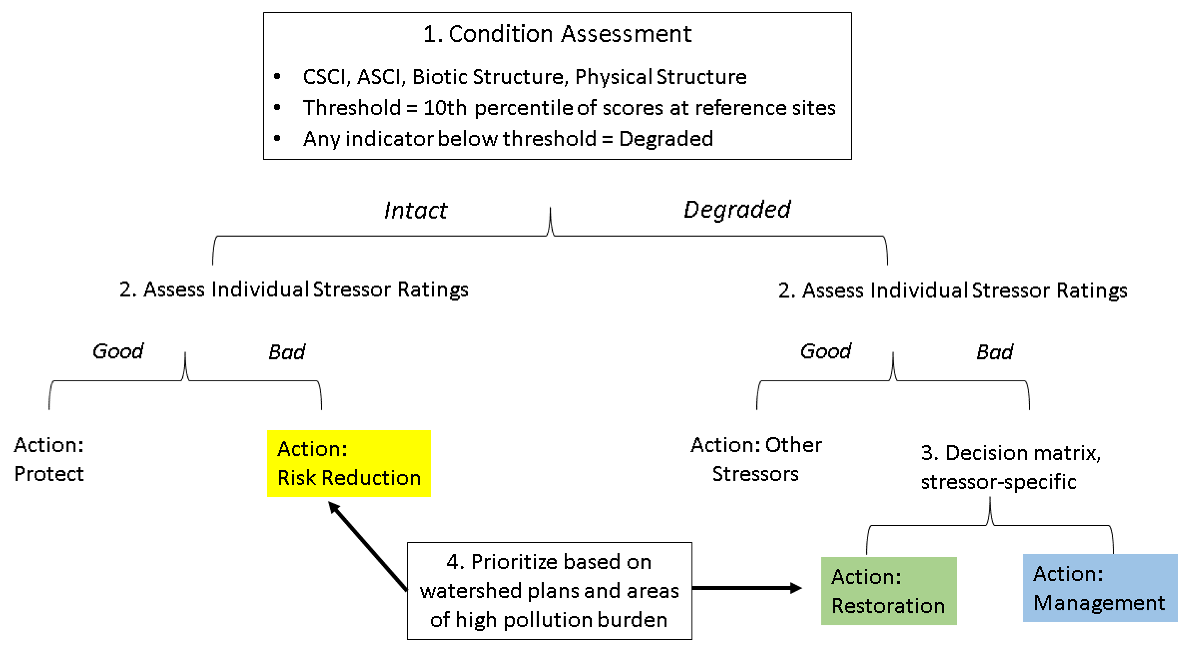
4.1. Utility of Tools for Watershed Prioritization

In this study, we developed a broadly applicable tool that can aid watershed managers in prioritizing protection, restoration, and management actions at a watershed scale to help promote overall watershed health. The prioritization tool leverages readily available data sources, such as statewide stream condition data based on ambient monitoring programs and USEPA’s national StreamCat database. As such, the tool can be easily applied to watersheds across diverse settings and landscapes using basic datasets that are available nationwide, such as USEPA’s National Rivers and Streams Assessment [28].

Developing this prioritization tool overcomes several traditional impediments to comprehensive watershed planning. First, results are provided at the reach scale, providing a more direct relationship with management actions. Other watershed prioritization tools use algorithms to provide results at the catchment scale (e.g., HUC 12), which requires assumptions or interpolation of management actions to specific locations [29,30]. In contrast, output at the reach scale allows managers to target their actions more easily to specific locations. Second, the tool provides specific recommendations tied to the most predominant stressors directly affecting biological condition at each stream location. Moving beyond general recommendations such as “management” or narrow outcomes such as “prioritization for non-point source control” [31] to a broader set of suggestions that remedy specific stressors helps support more directed and holistic watershed planning. This also increases the likelihood that stress amelioration will result in improvement of biological communities. Third, the tool is automated and can be easily applied to any watershed. This provides for rapid production of initial planning-level maps that can guide additional monitoring and subsequent in-depth analysis. This would be particularly useful for under-sampled areas where site-specific condition or stress data are not readily available. Because watershed planning can be an intensive process that involves data mining, compilation, synthesis, and manual analysis, the time and cost necessary to complete this process can often deter local watershed managers from attempting such comprehensive analysis, particularly in areas where resources or data are limited [30]. The availability of broadly applicable tool may lower these initial barriers to watershed planning. The tool can also supplement analysis in areas where local observations and field data are available by serving as an initial screening tool that can be verified with local data and by helping to provide information where field observations are not available. For example, the tool can be used to prioritize areas where formal causal assessment analysis should be conducted [32].

Parsimony in model development was based on a relatively sparse structure for the random forest modeling and a simple rule-based model for the management prioritization analysis. A sparse model structure contains the smallest number of covariates that might explain the greatest amount of variance in the dependent variable. Because this approach poses opportunities to inform decision-making, data collection, and protection and restoration activities in resource-restricted areas, it can be applied in a variety of settings regardless of the availability of local data. We recognize that streams and rivers are diverse systems with complex relationships to their biological communities and their surrounding societies, but our approach aims to balance this inherent complexity with a level of sparsity that best supports prioritization of management actions. The indices used in the random forest model development, ASCI, CSCI, and CRAM, are already examples of this balance of sparsity and complexity, combining several raw measures of biotic and physical conditions into a single metric [14,15,16]. By collapsing the axes of variability, this approach was designed to reduce the relative importance of variability in any one raw measure and enable trends in state-wide index datasets to emerge more clearly. For example, CRAM provided lower levels of discrimination because it is less sensitive to catchment-scale predictors, yet it provides a more direct estimation of habitat quality. These dichotomies can be offset by combining multiple condition indices. In the series of random forest models developed, we identified multiple shared environmental variables affecting stream condition, namely impervious and urban land cover as well as road density and crossings with streams which allows maximum leverage from limited data and improves overall relationships between stress and condition.

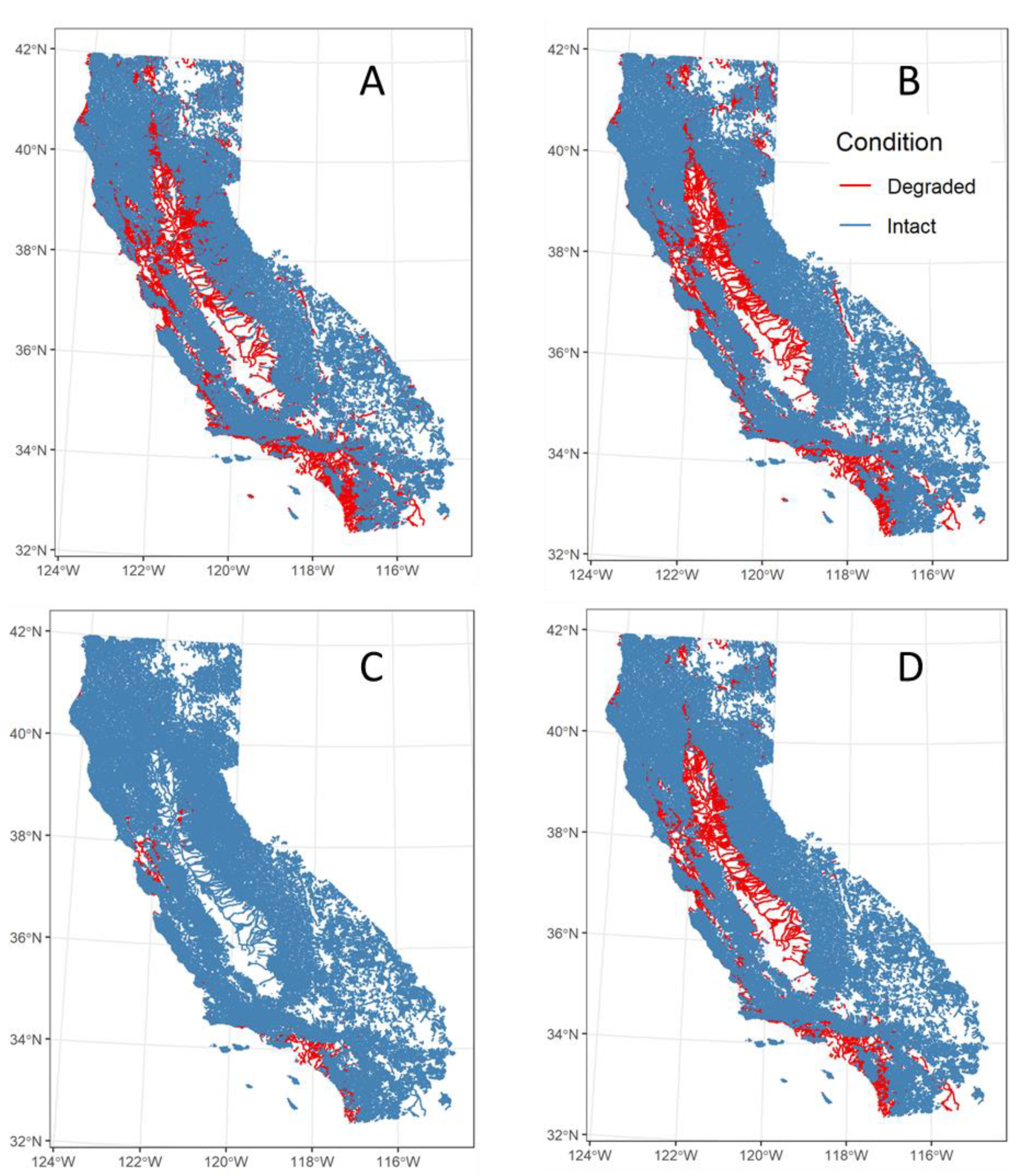
Results of random forest model development for condition assessment underscored the importance of long-term monitoring data in a variety of stream environments. Regions that had more data provided more information on which to develop the model and, as a result, their models explained a greater proportion of the variability in the data (Figures S2, S4, S6 and S8). Others have also called for increased monitoring as a critical need for future restoration efforts [33], and our model validation efforts highlighted the value of additional data, particularly in traditionally under-sampled regions. Similarly, monitoring the effect of future management actions on stream condition can provide the opportunity to verify the outputs of the prioritization tool and further refine it over time.

Tool acceptability was further enhanced through inclusive development of the rule-based model used to determine thresholds and match stressors with management actions. All rules and relationships in the models were co-developed and vetted through a statewide technical workgroup that included agency representatives and practitioners. This workgroup agreed on the approach to establishing thresholds, assigning stressors to mutually exclusive management categories and identifying specific actions to remedy specific stressors. Past studies have shown that agreement among experts on rule-based models can be considered equally reliable as models parameterized with empirical observations and results in higher reliability than subjective or “black-box” approaches [34,35]. Moreover, ensuring transparency in the development process, including important caveats and limitations of the tool improves confidence in the outcomes and helps achieve consensus on the appropriateness, logic, and defensibility of the products. Finally, the technical workgroup agreed that the recommendations provided by the tool should serve as suggestions to be further evaluated through site-specific analysis.

Reliance on StreamCat for stressor analysis provides a way to easily apply this approach nationwide using readily available data that are routinely updated. However, StreamCat is limited in that it only considers certain stressors and neglects potentially important stressors, such as grazing, timber harvest, some types of mines, and groundwater extraction. For example, groundwater extraction can severely impact riparian zone and can lead to catastrophic bank erosion and complete alteration of the stream course [36]. Such effects can be exacerbated by extended drought. Habitat descriptors based on conditions prevailing under years of non-extreme conditions may not be sensitive to severe drought, or effectively point toward the likely management needs associated with the disproportionate impacts under such conditions. StreamCat also under-represents the effects of aggregate extraction that can substantially alters stream structure. For example, historic aggregate mining in several of our pilot watersheds has been a major contributing factor to tens of meters of stream incision and water table decline, which has further affected stream conditions [37]. Finally, effects of episodic disturbance that can profoundly affects stream condition, such as wildfires and floods, are not represented in StreamCat.

Because the analysis was designed to apply at a state scale and relies on readily available geospatial data layers, it does not account for finer scale, more localized factors, such as local passage barriers or floodplain encroachment. Once the initial screening analysis using this approach is completed, it is important for users to account for finer-scale stress data before making final management decisions. This data may be available from datasets not represented in StreamCat, but from other regional or local sources.

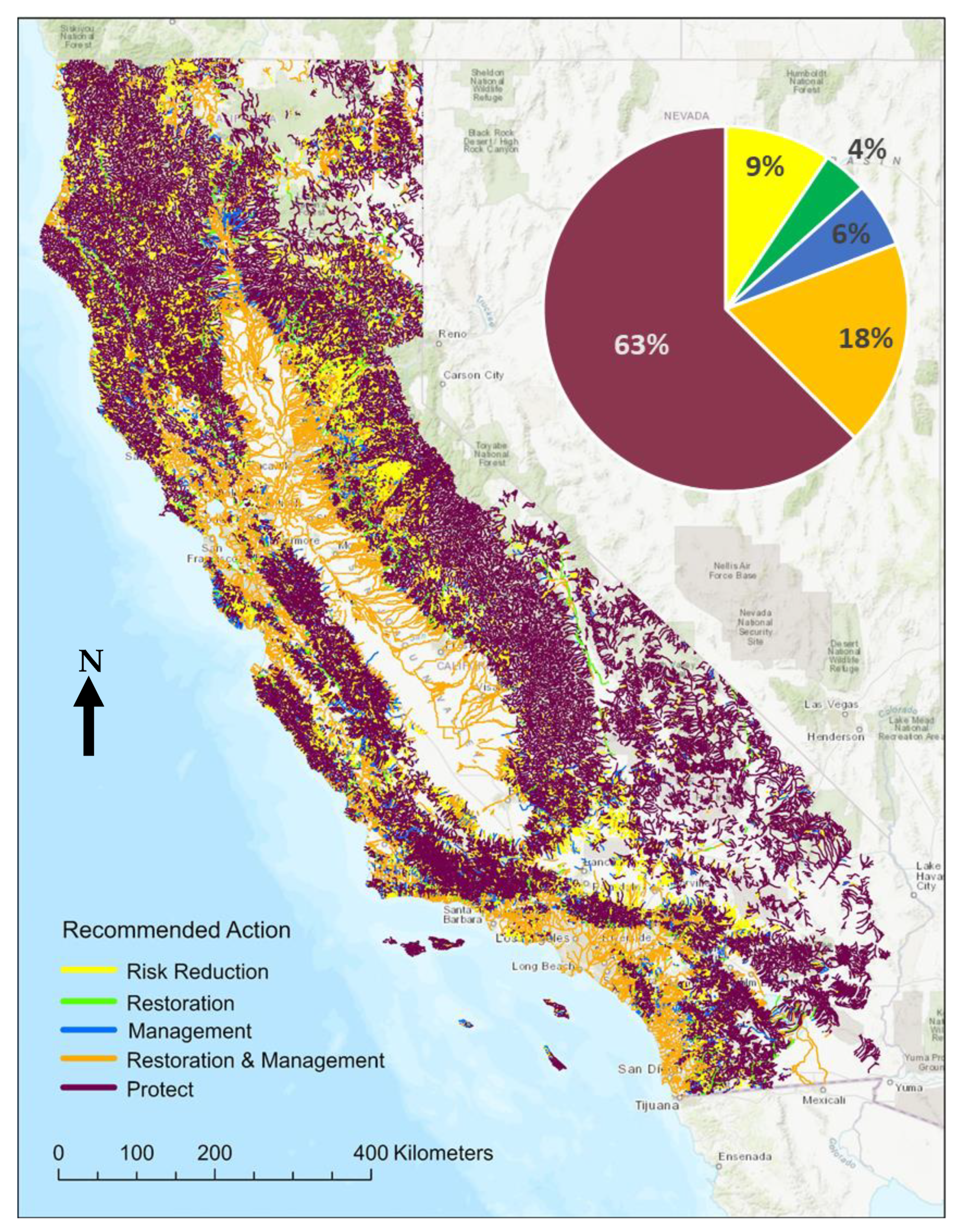
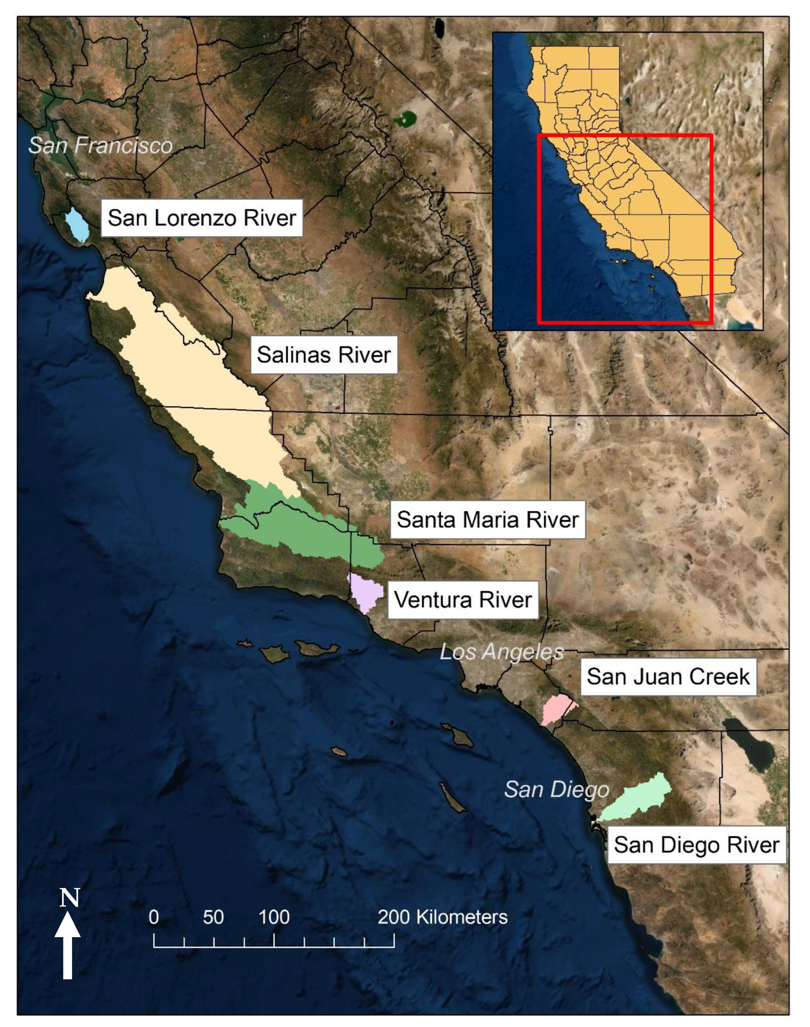
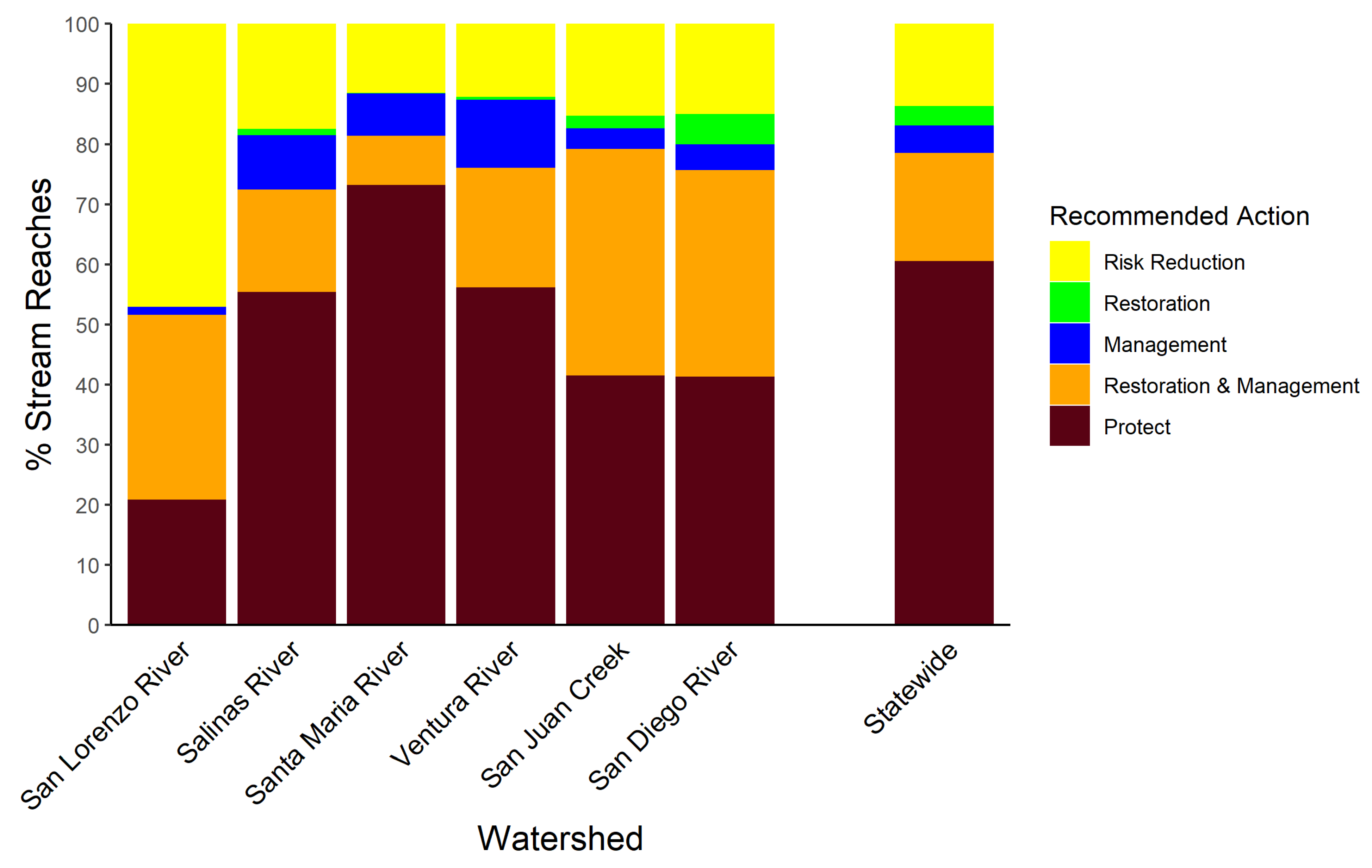
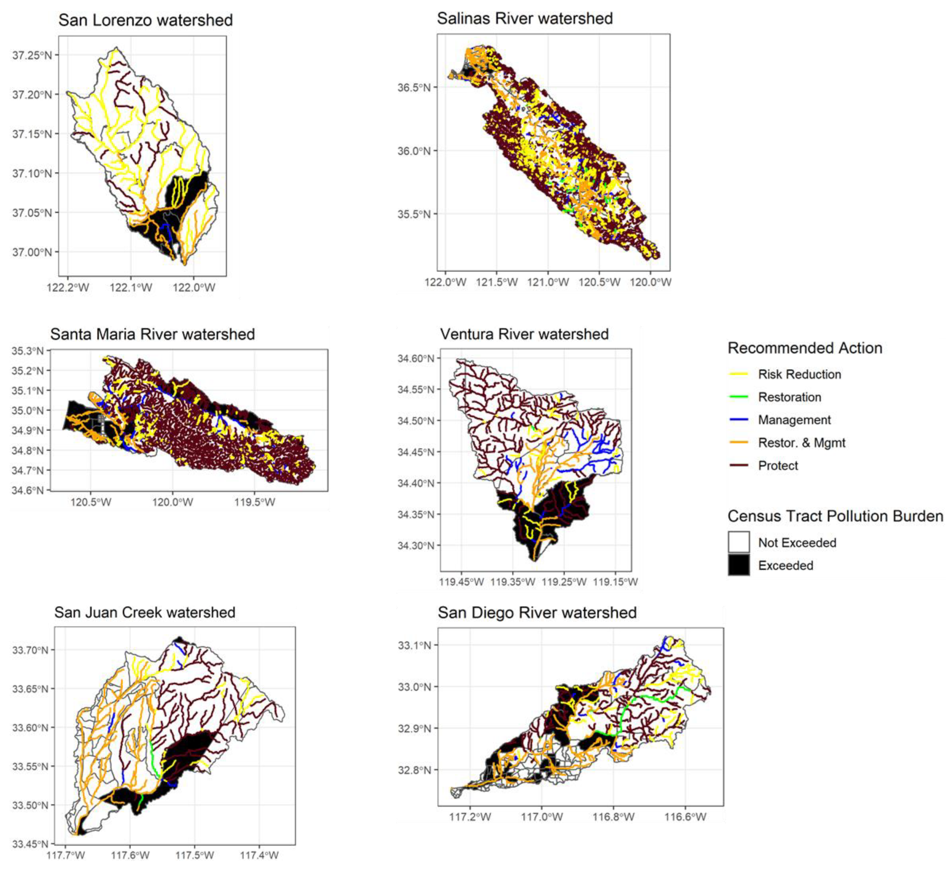
General patterns of recommended action statewide and in the six pilot watersheds corresponded to intensity of land uses in predictable ways. Moreover, tool performance was relatively consistent across the pilot watersheds, suggesting that it should be broadly applicable to all watersheds in the state. The exception was in the North Coast, where correlations were lowest. As noted, this may be due to sparser data. It may also reflect that these riparian systems are affected by variables other those tabulated by the five sets of standardized data, such as the influences of gorges on stream condition, the role of large wood logjams and the lingering effects of timber harvesting. In general, sites most in need of restoration and management were typically lower in the watershed where urban development is concentrated, or in the case of the Salinas River watershed, were associated with agricultural areas. High-quality sites recommended for protection were often at the interface between open space and urban or agricultural areas and were vulnerable due to elevated stressor levels. In contrast, sites recommended for no immediate action beyond continued protection were in more remote, less developed portions of the watershed. These sites should be monitored to determine if stress levels increase to a point where additional protective measures are recommended or if condition degrades to a level where restoration or management might be warranted. This is particularly important in consideration of globally induced changes in temperature, precipitation patterns and fire frequency which will have greater proportional effect on streams located in higher elevation, more natural portions of watersheds.

Most stream reaches in the state (63%) were in the protection category, suggesting that the prioritization tool was able to successfully identify reaches in greatest need of management intervention. However, it is important to keep in mind that all stream reaches are likely are already being affected by shifts in temperature and rainfall patterns associated with climate change. Moreover, future land use and resource management changes may pose additional threats. Therefore, every site has some degree of vulnerability and should be monitored for degradation from climate change, land use and resource management changes or a combination. Existing statewide monitoring programs could be used to periodically re-evaluate these “high quality” sites to determine their level of risk and whether their condition is declining.

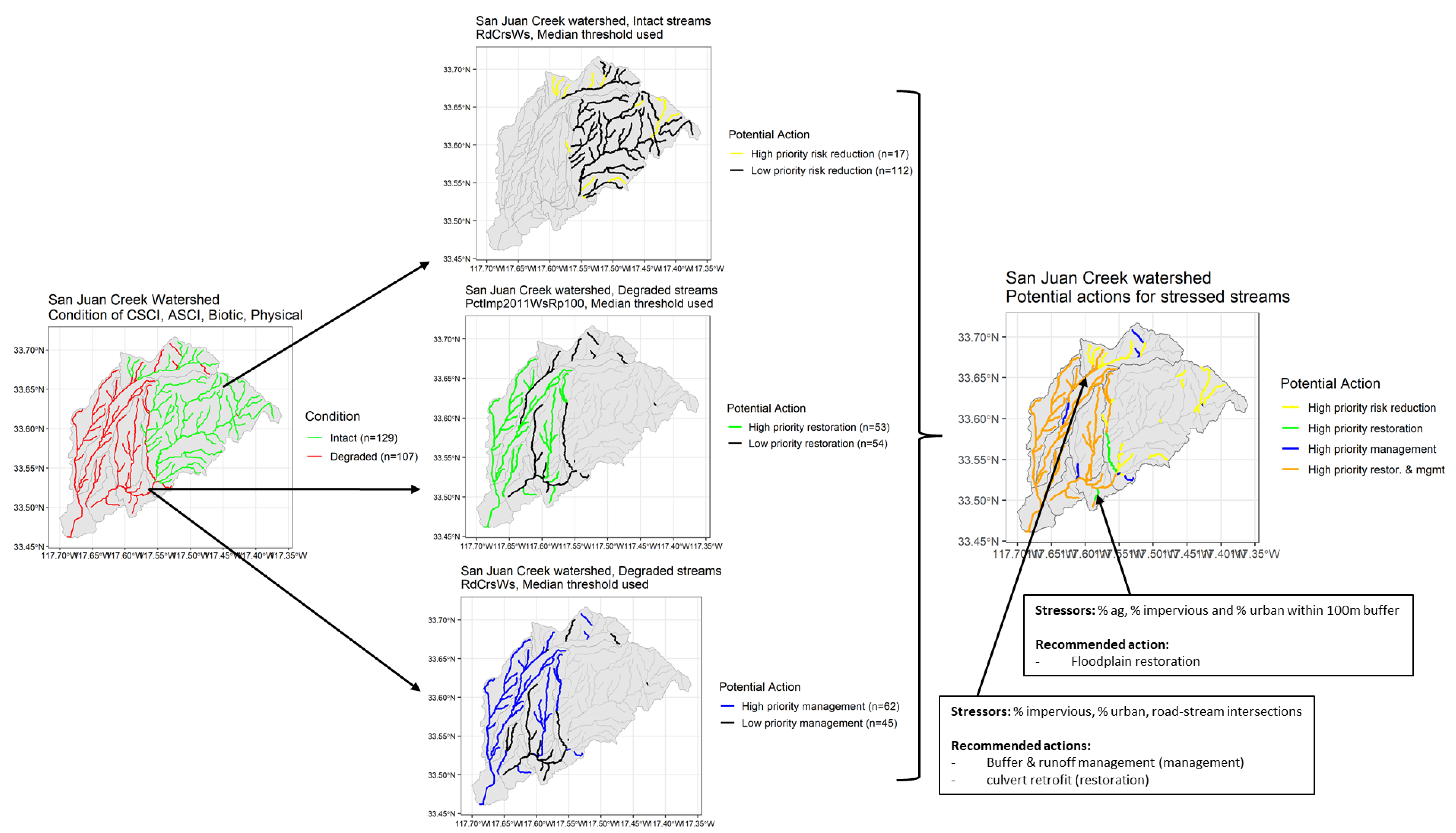
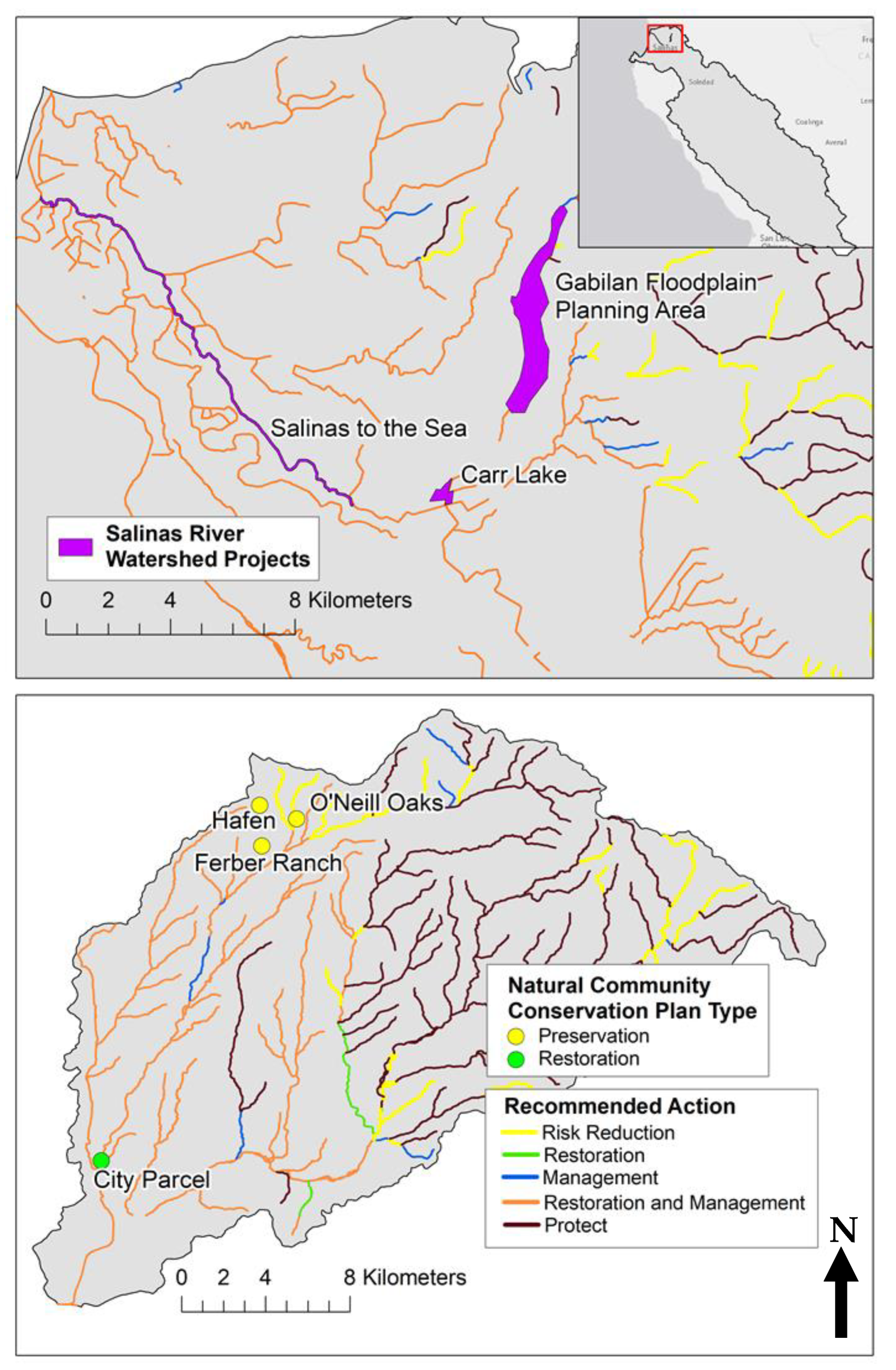
Unlike other prioritization tools, the results of this analysis also provide recommendations for specific actions to help remedy specific stressors (e.g., culvert retrofit in reaches with high density of road crossings). Observations during ground-truthing generally corroborated recommendations provided by the prioritization tool, suggesting that it can be broadly applied across watersheds in an automated manner to support initial watershed planning efforts. Coordination with local watershed plans could allow for additional prioritization through weighting of stressors based local priorities or ease of management intervention and provide opportunities s for leveraging of effort and investment to achieve multiple objectives associated with improving watershed health. Additional prioritization measures could also be imposed for lower stream reaches near the coast whose condition may be influenced by mouth conditions where they drain into the ocean. Closing patterns, and changes to those patterns due to armoring, artificial breaching, changing freshwater flows, and sea level rise can all affect condition in ways that are not detected through our analysis. These areas may also have additional environmental justice or community concerns that could affect how they are prioritized for management.

4.2. Importance of Accounting for Potentially Affected Communities

Regardless of model transparency, analytical results alone cannot always produce reliable restoration decisions [38]. Decisions need to include consideration of stakeholder values and community interests and needs. These communities are often closely related to their local rivers and streams, and they will have different priorities and values based on both cognitive and emotional perspectives. Many areas may have religious or cultural significance for indigenous cultures that should be integrated into watershed planning. In general, restoration efforts have a propensity to prioritize restoration in natural areas because they are easier to regain ecological functions. However, this narrow ecological and engineering focus contributes to the exclusion of restoration in areas that can provide benefits to communities that often lack access to “natural areas” for recreational and educational benefits [39].

Research in environmental justice has repeatedly noted that scientific information by itself is not sufficient to indicate the ideal location for projects. Rather, a full consideration of the expected benefits, and where they accrue, is also important. This can best be accomplished by expanding restoration considerations beyond the stream itself to the characteristics and needs of the surrounding communities. In this study, we attempted to include environmental justice considerations into restoration prioritization using the CalEnviroScreen dataset. CalEnviroScreen data supplies California communities with environmental, health, and socioeconomic data pertaining to each census tract, allowing the community to examine which regions have the highest levels of pollution and population burdens. Our preliminary analysis showed little correlation between the CalEnviroScreen indicators and indicators of stream condition (e.g., ASCI, CSCI, and CRAM). At one level, this suggests that the two assessments are measuring different things (stream condition vs. condition of the surrounding community). At another level, this suggests a potential incongruence between ecological and social needs. By prioritizing streams in areas with the highest overall pollution burdens, we can begin to better incorporate the needs of under-resourced communities into the restoration prioritization process. Full integration of ecological and social issues will ultimately require development of new indicators that more directly measure ecological aspects of streams that provide social benefit, such as access to recreational opportunities. Consideration of the broader social benefits of restoration and management was beyond the scope of this study but is an important area for future investigation.

5. Conclusions

In this study, we set out to address the call for new methods in stream restoration prioritization [40], and we successfully developed a series of condition classification models that make use of large spatio-temporal datasets and recently developed indices to generate sparse model structures well suited for informing prioritization measures. The tools produced in this study provide a parsimonious way to spatially prioritize specific management actions across a watershed, and they provide a series of discrete activities aimed at collectively improving watershed health. This tool is most appropriately used to support preliminary screening-level analysis of priority locations and actions to help restore healthy watersheds. It will be most useful in data-poor areas that lack a critical mass of detailed site-specific investigations. Moreover, the outcomes likely represent a “best-case scenario” of condition. Holistic watershed management requires consideration of the processes and interactions across the watershed such as sediment transport and continuity for wildlife movement [41,42]. Such finer-scale analysis often reveals additional stressors that affect condition, but also inform more directed management actions. Advances in spatial modeling can be applied to future analysis to further prioritize sites for protection, restoration, or management based on their importance for maintaining or restoring corridors or linkages or aquatic or riparian organisms [43]. Similarly, areas that provide processes such as aquifer recharge and sediment generation could be prioritized based on their position in the watershed. For example, areas that provide coarse sediment supply necessary to maintain geomorphic stability could be prioritized for protection, whereas key sediment transport areas could be prioritized for restoration [44]. Reaches likely to have been affected by episodic events, such as post-fire sedimentation or fire-flood disturbance, can be identified by overlaying polygons of fire perimeters both to assess whether adjustments in reach data may be needed, or to simply flag certain reaches as being prone to occasional pulses of sediment and nutrients [45,46]. Including such positional considerations in future model or tool development would provide for a more complete and nuanced approach to prioritizing actions to achieve healthy watersheds.

References

1. Jones, K.B.; Slonecker, E.T.; Nash, M.S.; Neale, A.C.; Wade, T.G.; Hamann, S. Riparian habitat changes across the continental United States (1972–2003) and potential implications for sustaining ecosystem services. Landsc. Ecol. 2010, 25, 1261–1275. [Google Scholar] [CrossRef]
2. Sheehan, L.; Tasto, R. The status of habitats and water quality in California’s coastal and marine environment. In California’s Living Marine Resources: A Status Report; Leet, W.S., Dewees, C.M., Klingbeil, R., Larson, E.J., Eds.; California Department of Fish and Game: Sacramento, CA, USA, 2001; pp. 29–45. [Google Scholar]
3. NRC (National Research Council). Upstream: Salmon and Society in the Pacific Northwest Washington, D.C.; National Academy Press: Cambridge, MA, USA, 1996. [Google Scholar]
4. U.S. Environmental Protection Agency. Healthy Watersheds Initiative: National Framework and Action Plan; EPA: Washington DC, USA, 2011; Publication Number: EPA 841-R-11-005. [Google Scholar]
5. Allan, J.D.; Abell, R.; Hogan, Z.E.B.; Revenga, C.; Taylor, B.W.; Welcomme, R.L.; Winemiller, K. Overfishing of inland waters. BioScience 2005, 55, 1041–1051. [Google Scholar] [CrossRef] [Green Version]
6. Harrison, I.J.; Stiassny, M.L.J. The quiet crisis: A preliminary listing of freshwater fishes of the world that are extinct or “missing in action”. Extinctions Near Time R MacPhee 1999, 271–331. [Google Scholar] [CrossRef]
7. Meybeck, M. The global change of continental aquatic systems: Dominant impacts of human activities. Water Sci. Technol. 2004, 49, 73–83. [Google Scholar] [CrossRef]
8. Poff, N.L.; Allan, J.D.; Bain, M.B.; Karr, J.R.; Prestegaard, K.L.; Richter, B.D.; Sparks, R.E.; Stromberg, J.C. The natural flow regime. BioScience 1997, 47, 769–784. [Google Scholar] [CrossRef]
9. Abell, R.; Allan, J.D.; Lehner, B. Unlocking the potential of protected areas for freshwaters. Biol. Conserv. 2007, 134, 48–63. [Google Scholar] [CrossRef]
10. Bernhardt, E.S.; Palmer, M.A.; Allan, J.D.; Alexander, G.; Barnas, K.; Brooks, S.; Carr, J.; Clayton, S.; Dahm, C.; Follstad-Shah, J.; et al. Synthesizing US River restoration efforts. Science 2005, 308, 636–637. [Google Scholar] [CrossRef]
11. Flotemersch, J.E.; Leibowitz, S.G.; Hill, R.A.; Stoddard, J.L.; Thoms, M.C.; Tharme, R.E. A watershed integrity definition and assessment approach to support strategic management of watersheds. River Res. Appl. 2016, 32, 1654–1671. [Google Scholar] [CrossRef]
12. Buto, S.G.; Anderson, R.D. NHDPlus High Resolution (NHDPlus HR)—A Hydrography Framework for the Nation: U.S. Geological Survey Fact Sheet 2020–3033; USGS: Reston, VA, USA, 2020; p. 2. [Google Scholar] [CrossRef]
13. Hill, R.A.; Weber, M.H.; Leibowitz, S.G.; Olsen, A.R.; Thornbrugh, D.J. The Stream-Catchment (StreamCat) Dataset: A database of watershed metrics for the conterminous United States. JAWRA J. Am. Water Resour. Assoc. 2016, 52, 120–128. [Google Scholar] [CrossRef]
14. Mazor, R.D.; Rehn, A.C.; Ode, P.R.; Engeln, M.; Schiff, K.C.; Stein, E.D.; Gillett, D.J.; Herbst, D.B.; Hawkins, C.P. Bioassessment in complex environments: Designing an index for consistent meaning in different settings. Freshw. Sci. 2016, 35, 249–271. [Google Scholar] [CrossRef]
15. Theroux, S.; Mazor, R.D.; Beck, M.W.; Ode, P.R.; Stein, E.D.; Sutula, M. Predictive biological indices for algae populations in diverse stream environments. Ecol. Indic. 2020, 119, 106421. [Google Scholar] [CrossRef]
16. California Wetlands Monitoring Workgroup (CWMW). California Rapid Assessment Method (CRAM) for Wetlands, Version 6.1. 2013; p. 67. Available online: https://www.cramwetlands.org/ (accessed on 23 March 2022).
17. Liaw, A.; Wiener, M. Classification and Regression by Random Forest, R News. 2002. Available online: https://CRAN.R-project.org/doc/Rnews/ (accessed on 23 March 2022).
18. Kuhn, M.; Wickham, H. Tidymodels: A Collection of Packages for Modeling and Machine Learning Using tidyverse Principles. 2020. Available online: https://www.tidymodels.org (accessed on 23 March 2022).
19. Wickham, H.; Averick, M.; Bryan, J.; Chang, W.; McGowan, L.D.; François, R.; Grolemund, G.; Hayes, A.; Henry, L.; Hester, J.; et al. Welcome to the Tidyverse. J. Open Source Softw. 2019, 4, 1686. [Google Scholar] [CrossRef]
20. Ode, P.R.; Kincaid, T.M.; Fleming, T.; Rehn, A.C. Ecological Condition Assessments of California’s Perennial Wadeable Streams: Highlights from the Surface Water Ambient Monitoring Program’s Perennial Streams Assessment (PSA) (2000–2007). In A collaboration between the State Water Resources Control Board’s Non-Point Source Pollution Control Program (NPS Program), Surface Water Ambient Monitoring Program (SWAMP); California Department of Fish and Game Aquatic Bioassessment Laboratory: Rancho Cordova, CA, USA, 2011. [Google Scholar]
21. Kuhn, M. Caret: Classification and Regression Training. 2021. Available online: https://CRAN.R-project.org/package=caret (accessed on 1 September 2020).
22. Fong, L.S.; Stein, E.D.; Ambrose, R.F. Development of restoration performance curves for streams in southern California using an integrative condition index. Wetlands 2017, 37, 289–299. [Google Scholar] [CrossRef]
23. Beck, M.W.; Mazor, R.D.; Theroux, S.; Schiff, K.C. The Stream Quality Index: A multi-indicator tool for enhancing environmental management. Environ. Sustain. Indic. 2019, 1, 100004. [Google Scholar] [CrossRef]
24. California Environmental Protection Agency (CalEPA) and Office of Environmental Health Hazard Assessment (OEHHA). CalEnviroScreen 3.0. Update to the California Communities Environmental Health Screening Tool. 2017; p. 168. Available online: https://oehha.ca.gov/media/downloads/calenviroscreen/report/ces3report.pdf (accessed on 23 March 2022).
25. National Land Cover Database (NLCD). 2016. Available online: https://www.mrlc.gov/national-land-cover-database-nlcd-2016 (accessed on 23 March 2022).
26. ICF. Orange County Transportation Authority M2 Natural Community Conservation Plan/Habitat Conservation Plan; Administrative Final. October. (ICF 00536.10.) San Diego, CA. Technical Report; Orange County Transportation Authority: Orange, CA, USA, 2016. [Google Scholar]
27. Orange County Department of Public Works. South Orange County Watershed Management Area 2018 Integrated Regional Water Management Plan; Orange County Department of Public Works: Orange County, FL, USA, 2018. [Google Scholar]
28. U.S. Environmental Protection Agency. National Rivers and Streams Assessment 2013–2014: A Collaborative Survey. EPA 841-R-19-001. Washington, DC. 2020. Available online: https://www.epa.gov/national-aquatic-resource-surveys/nrsa (accessed on 23 March 2022).
29. Jaiswal, R.K.; Ghosh, N.C.; Galkate, R.V.; Thomas, T. Multi Criteria Decision Analysis (MCDA) for watershed prioritization. Aquat. Procedia 2015, 4, 1553–1560. [Google Scholar] [CrossRef]
30. Rahmati, O.; Samadi, M.; Shahabi, H.; Azareh, A.; Rafiei-Sardooi, E.; Alilou, H.; Melesse, A.M.; Pradhan, B.; Chapi, K.; Shirzadi, A. SWPT: An automated GIS-based tool for prioritization of sub-watersheds based on morphometric and topo-hydrological factors. Geosci. Front. 2019, 10, 2167–2175. [Google Scholar] [CrossRef]
31. Peacock, B.C.; Hikuroa, D.; Morgan, T.K.K.B. Watershed-scale prioritization of habitat restoration sites for non-point source pollution management. Ecol. Eng. 2012, 42, 174–182. [Google Scholar] [CrossRef]
32. Schiff, K.; Gillett, D.J.; Rehn, A.; Paul, M. Causal Assessment Evaluation and Guidance for California. Southern California Coastal Water Research Project, Technical Report #750. 2015. Available online: https://www.sccwrp.org/ (accessed on 23 March 2022).
33. Wohl, E.; Lane, S.N.; Wilcox, A.C. The science and practice of river restoration. Water Resour. Res. 2015, 51, 5974–5997. [Google Scholar] [CrossRef] [Green Version]
34. Weisberg, S.B.; Thompson, B.; Ranasinghe, J.A.; Montagne, D.E.; Cadien, D.B.; Dauer, D.M.; Diener, D.R.; Oliver, J.S.; Reish, D.J.; Velarde, R.G.; et al. The level of agreement among experts applying best professional judgment to assess the condition of benthic infaunal communities. Ecol. Indic. 2008, 8, 389–394. [Google Scholar] [CrossRef]
35. Teixeira, H.; Borja, A.; Weisberg, S.B.; Ranasinghe, J.A.; Cadien, D.B.; Dauer, D.M.; Dauvin, J.C.; Degraer, S.; Diaz, R.J.; Grémare, A.; et al. Assessing coastal benthic macrofauna community condition using best professional judgement—Developing consensus across North America and Europe. Mar. Pollut. Bull. 2010, 60, 589–600. [Google Scholar] [CrossRef]
36. Kondolf, G.M.; Curry, R. The role of Riparian Vegetation in Channel Bank Stability: Carmel River, California. In Proceedings of the California Riparian Symposium, September 1981; University of California Press: Davis, CA, USA, 1984. [Google Scholar]
37. Hecht, B.; Brown, S.; Mallory, B. Geomorphologic Factors Affecting Sediment Generation and Transport Under Pre- and Post-Urbanization Conditions at Rancho Mission Viejo and in the San Juan and San Mateo Watersheds, Orange County, California, USA; Project Number 99058. Prepared for Rancho Mission Viejo; Balance Hydrologics, Inc.: Berkeley, CA, USA, 2004; p. 43. [Google Scholar]
38. Failing, L.; Gregory, R.; Higgins, P. Science, Uncertainty, and Values in Ecological Restoration: A Case Study in Structured Decision-Making and Adaptive Management. Restor. Ecol. 2013, 21, 422–430. [Google Scholar] [CrossRef]
39. Moran, S. Cities, Creeks, and Erasure: Stream Restoration and Environmental Justice. Environ. Justice 2010, 3, 61–69. [Google Scholar] [CrossRef]
40. Palmer, M.; Ruhi, A. Linkages between flow regime, biota, and ecosystem processes: Implications for river restoration. Science 2019, 365, eaaw2087. [Google Scholar] [CrossRef] [PubMed] [Green Version]
41. Frissell, C.A.; Liss, W.J.; Warren, C.E.; Hurley, M.D. A hierarchical framework for stream habitat classification: Viewing streams in a watershed context. Environ. Manag. 1986, 10, 199–214. [Google Scholar] [CrossRef]
42. Jones, N.E.; Schmidt, B.J. Tributary effects in rivers: Interactions of spatial scale, network structure, and landscape characteristics. Can. J. Fish. Aquat. Sci. 2016, 74, 503–510. [Google Scholar] [CrossRef]
43. Burcher, C.L.; Valett, H.; Benfield, E.F. The Land-Cover Cascade: Relationships Coupling Land and Water. Ecology 2007, 88, 228–242. [Google Scholar] [CrossRef] [Green Version]
44. Booth, D.B.; Leverich, G.; Downs, P.W.; Dusterhoff, S.; Araya, S. A Method for Spatially Explicit Representation of Sub-watershed Sediment Yield, Southern California, USA. Environ. Manag. 2014, 53, 968–984. [Google Scholar] [CrossRef]
45. Hecht, B. Sequential changes in physical conditions affecting aquatic habitat in the upper Carmel River, California, following the Marble-Cone Fire of August 1977. In Proceedings of the California Riparian Symposium, September 1981; University of California Press: Davis, CA, USA, 1984; pp. 134–142. [Google Scholar]
46. Mazor, R.D.; Gillett, D.J.; Schiff, K.C.; Ritter, K.; Stein, E.D. Ecological Condition of Watersheds in Coastal Southern California: Progress Report of the Stormwater Monitoring Coalition’s Stream Monitoring Program First Year (2009). In Technical Report 639; Southern California Coastal Water Research Project: Costa Mesa, CA, USA, 2011. [Google Scholar]
Figure 1. Process used to prioritize stream reaches for protection, restoration, or management. Intact sites with low stress should be protected and monitored. Degraded sites where median stress values did not exceed thresholds should be monitored and investigated for other stressors.
Water 14 01375 g001
Figure 2. Location of the six test watersheds used to ground truth the watershed prioritization methods.
Water 14 01375 g002
Figure 3. Predicted condition index results based on random forest model outputs for statewide stream reaches in California. Panels (AD) refer to the ASCI, CSCI, CRAM biotic structure, and CRAM physical structure indices, respectively. For each index, stream reaches were classified as “degraded” if the normalized index score was less than the 10th percentile value from reference sites.
Water 14 01375 g003
Figure 4. Recommended actions for all stream reaches in California based on outputs of the watershed prioritization analysis. An interactive map with reach-specific information can be found at: https://gamma-data-portal-sccwrp.hub.arcgis.com/maps/watershed-prioritization-recommended-actions-2021-summary/explore (accessed on 23 March 2022).
Water 14 01375 g004
Figure 5. Example integration of watershed prioritization analysis for the San Juan Creek watershed.
Water 14 01375 g005
Figure 6. Proportion of recommended actions within each of the six test watersheds, and statewide.
Water 14 01375 g006
Figure 7. Recommended actions for each of the six pilot watersheds, including areas with high pollution burden that could be prioritized to benefit communities disproportionately affected by pollution. Larger versions of these maps are provided in Supplemental Material S3.
Water 14 01375 g007
Figure 8. Priority areas in the Salinas River Watershed (top panel) and San Juan Creek Watershed (bottom panel) based on opportunities to leverage efforts with existing watershed conservation and restoration plans.
Water 14 01375 g008